Quantum and Classical Methods to Improve the Efﬁciency of Infocom Systems

(1)

z

Quantum and Classical Methods to Improve the Efficiency of Infocom Systems

DsC Thesis

S´andor IMRE

Budapest University of Technology and Economics

Department of Telecommunications

(2)

how to endure to the end.

Sandor Imre

P.S. And of course to my children Sanyus, Marci, Orsi, Andris and their mother Adel.

(3)

Acknowledgments

The author gratefully acknowledges the comments, helpful advices and permanent encour- agement of Prof. L´aszl´o Pap. Pressure and interest of colleagues and students of Mobile Communication and Computing Laboratory were very motivating.

iii

(4)

List of Figures

1.1 Moore’s Law 3

3.1 Circuit implementing the Grover operator 13

3.2 Geometrical interpretation of the Grover operator 14 3.3 The matching condition between φ andθ with and without correction

assumingΩ = 0.5, ^Ω₂^γ = 0.0001,Λγ = 0.004,Λ = 0.004 23 3.4 Geometrical interpretation of the generalized Grover iteration 24 3.5 Different possible interpretations of|γ1i⁰ 25 3.6 Υvs. θassumingΩ = 0.5, ^Ω₂^γ = 0.0001,Λ_γ = 0.004,Λ = 0.004 25 3.7 Number of iterationslsvs. θassuming the matching condition is fulfilled

andΩ = 0.0001, ^Ω₂^γ = 0.0001,Λγ = Λ = 0 27

4.1 Quantum counting circuit 31

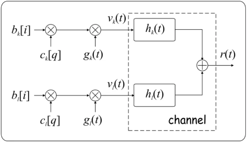
5.1 DS-CDMA transmitter and channel 40

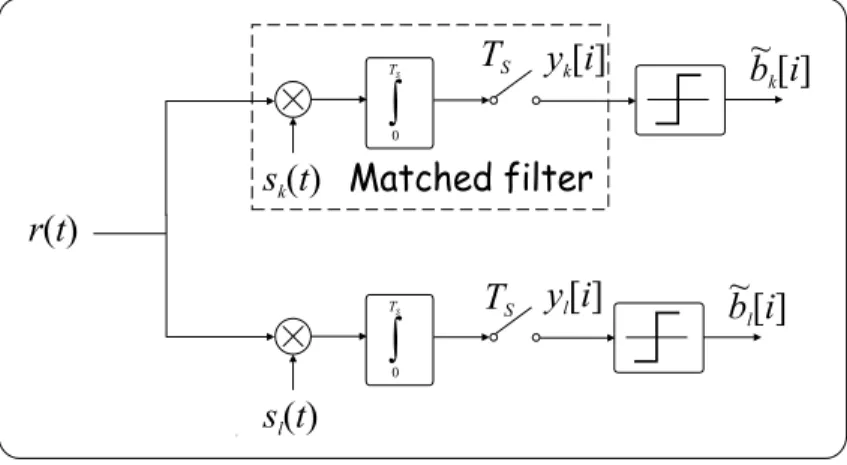
5.2 Single-user DS-CDMA detector with matched filter, idealistic case 44

5.3 Multi-user DS-CDMA detector 44

5.4 Quantum error probability log₁₀( ˘Pε) vs. number of required additional

qbitsp 47

5.5 System concept of quantum counting based multi-user DS-CDMA detector 47

viii

(9)

5.6 The structure of the index register 47 7.1 System model with reference and neighboring cells 54

7.2 Average distances for different cell types 60

8.1 Geometric interpretation of CAC 62

8.2 Effective bandwidth based and dynamic separation surfaces 65 11.1 System model with reference and neighboring cells in case of soft handover 86 11.2 System model with reference and neighboring cells for downlink 87 12.1 Accepted network states vs. air interface capacity in case of static

comparison 89

12.2 Number of accepted calls as a function ofλ2 90

12.3 Ratio of accepted calls vs. call attempts as a function ofλ2 90 12.4 Number of required iterations as a function ofd 92

(10)

Acronyms

BSi Base Station in celli BER Bit Error Ratio

BPSK Binary Phase Shift Keying CAC Call Admission Control

CDMA Code Division Multiple Access DES Data Encryption Standard DCT Discrete Cosine Transform DFT Discrete Fourier Transform

DS-CDMA Direct Sequence-Code Division Multiple Access FDMA Frequency Division Multiple Access

FFT Fast Fourier Transform HLR Home Location Register

GC Guard Channel

GSM Global System for Mobile communications GUT Great Unified Theory

IQFT Inverse Quantum Fourier Transform LMGF Logarithmic Moment Generator Function LSB Least Significant Bit

MSB Most Significant Bit

x

(11)

MAC Medium Access Control MAI Multiple Access Interference MAP Maximum A Posteriori

ML Maximum Likelihood

MLS Maximum Likelihood Sequence MUD Multiuser Detection

NMR Nuclear Magnetic Resonance pdf probability density function PLMN Public Land Mobile Networks

PG Processing Gain

QC Quantum Computation/Quantum Computing QFT Quantum Fourier Transform

QoS Quality of Service

QMUD Quantum based Multiuser Detection r.v. random variable

SDM Space Division Multiplexing SDMA Space Division Multiple Access SIM Subscriber Identity Module SIR Signal to Interference Ratio SNR Signal to Noise Ratio

SIDR Signal to Interference Density Ratio SRM Square-Root Measurement

SS Spread Spectrum

TDM Time Division Multiplexing TDMA Time Division Multiple Access

UMTS Universal Mobile Telecommunication System URL Uniform Resource Locator

UTC User Traffic Control

WCDMA Wideband Code Division Multiple Access WLAN Wireless Local Area Network

WWW World Wide Web

(12)

Notations

˜

a Measured/estimated value of variablea

˘

a Technical constrain/demand for variablea, e.g. amust be less thana˘

∀ for all

j √

−1

|·i Vector representing a quantum state, its coordinates are probability amplitudes

x Traditional vector, e.g. x∈ {0,1}ⁿrefers to the vector representation ofn-bit binary numbers

|·iN State of anN-dimensional quantum register, i.e. the qregister contains n = ld(N)qubits

|0i Special notion for the more than one-qbit zero computational basis vector to distinguish it from the single qbit|0i

U Operator

U^⊗ⁿ n-qbit (2ⁿ-dimensional) operator U Matrix of operatorU

P(α) Phase gate with matrix

1 0 1 e^jα

H Hadamard gate with matrix √¹ 2

1 1 1 −1

X Pauli-X(bit-flip) gate with matrix

0 1 1 0

Y Pauli-Y gate with matrix

0 −j j 0

xii

(13)

Z Pauli-Z (phase-flip) gate with matrix

1 0 0 −1

⊗ Tensor product, this notation is often omitted, it is used only if the tensor product operation has to be emphasized

⊕ Modulo 2 addition

(·)^∗ Complex conjugate h·|·i Inner product

|·ih·| Outer product

† Adjoint

(·)^T Transpose

∗ Convolution

, Definition

≡ Equivalence

∧ Logical AND operator

∨ Logical OR operator

| Logical IF operator Z Set of integer numbers Z₂ ≡ {0,1}Set of binary numbers (Z₂)ⁿ Set ofn-bit binary numbers

Z_N Set of positive integer numbers between0and(N −1), i.e. set belonging to the moduloN additive group

Z⁺ Set of natural numbers i.e. positive integer numbers Z− Set of negative integer numbers

Z^∗

p Set of positive integers belonging to the moduloN multiplicative group C Set of complex numbers

ld(·) Logarithmus dualis,log₂(·)

d·e Smallest integer greater than or equal to a number b·c Greatest integer less than or equal to a number b·e Rounds to the nearest integer

gcd(a, b) Greatest common divisor ofaandb fQ(q) Probability density function of r. v. Q f(x) Function continuous inx

f[x] Function discrete inx

(14)

<(x) Real part of complex numberx

=(x) Imaginary part of complex numberx

#(·) Number of, counts the occurrence of its argument Thin line Quantum channel

Thick line Classical channel

Special indices applied in chapters devoted to WCDMA

Remark: Generally in case of any variable with indexesij is written only with index j means that it represents one variable from class j and this variable is the same for all terminals in the given class.

k^#= 1...K:sequence number of base stations (cells) in the interference region.

k= 1..K_k^#:cell IDs of CAC region of base stationk^#. j = 1..J: traffic classes.

h: auxiliary variable ofj.

i= 1..N_jk^#:refers to terminalifrom classjlocated in cell andk^#. l: auxiliary variable ofi.

t= 1..∞: sequence number of actual call event (arrival or termination).

(15)

Motto

"It takes a thousand men to invent a telegraph, or a steam engine, or a phonograph, or a photograph, or a telephone, or any other Important thing – and the last man gets the credit and we forget the others. He added his little mite – that is all he did."

Mark Twain

xv

(16)

1 Motivations

"Navigare necesse est!"¹

Ancient Romans

If one compares wired and wireless/mobile communications several differences can be recognized in such fields as security, power consumption, medium access, channel behavior etc. However, the most differently handled resource is bandwidth. In case of wired networks link capacity can overcome almost any limitations by deploying optical fibres. In contrast wireless bandwidth is strongly restricted thanks to on one hand regulation and on the other hand to enormously large licence prices. Therefore, spectral efficiency is one of the most significant key parameters of every mobile system. Spectrally efficient wireless solutions are fairly complex, they consist of techniques applied in physical and data link layers.

Call Admission Control (CAC) methods are very important since they ensure Quality of Service (QoS) while increasing spectral efficiency so they provide tradeoff between two competing aspects. Quantum computing and communications just appeared in infocom systems. They offer completely new principles and techniques which are not available in classical computing and communications. Therefore, it is worth attacking wide range of computationally complex problems of infocom systems from data base searching to useful signal detection in multiuser environment.

1"Shipping is a must!"

1

(17)

1.1 QUANTUM COMPUTERS AND COMPUTING

"Man is the best computer we can put aboard a spacecraft... and the only one that can be mass-produced with unskilled labor.

Wernher von Braun

In order to understand the importance of quantum computing and communications let us focus shortly on the history of computers, computing and communications. The most important steps towards an electronic computer were done during World War II when the large number of calculations in the Manhattan project required an elementary new equipment which is fast enough and adaptive (programmable). Many clever scientist were engaged with this problem. We mention here among them the polymath Neumann because he played important role in quantum mechanics as well but at this moment we say thank to him for the invention of the ’control by stored program’ principle². This principle combined with the vacuum tube hardware formed the basis of the first successful computers³. Unfortunately the tubes strongly limited the possibilities of miniaturization hence first computers filled up a whole room, which strongly restricted their wide applications. Therefore scientists paid distinguished attention to the small-scale behavior of matter. Fortunately the invention of semiconductors and the appearance of the transistor in 1948 by Bardeen, Brattain and Schockley open the way to personal computers and other handhold equipment.

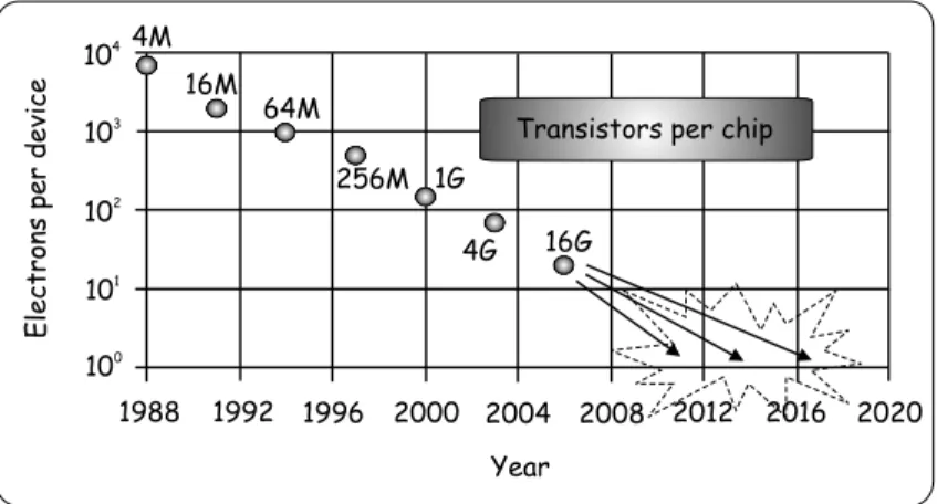
One day in 1965 when Gordon Moore from Intel was preparing his talk and started to draw a plot about the performance of memory chips suddenly he observed an interesting rule called Moore’s Law. As it is depicted in Fig. 1.1 he concluded that since the invention of the transistor the number of transistors per chip roughly doubled every 18-24 months, which means an exponential increase in the computing power of computers. Although it was an empirical observation without theoretical proof the Law seems to be still valid nowadays.

However, similarly to the case of steam engine farseeing experts tried to determine the future of this technology. They estimate serious problems around 2015. What reasons may stand behind this prophecy?

No matter how surprisingly it sounds this trend can be traced back simply to drawing lines. The growth in processors’ performance is due to the fact that we put more and more transistors on the same size chip. This requires smaller and smaller transistors, which can be achieved if we are able to draw thinner and thinner – even much thinner than a hair – lines onto the surface of a semiconductor disc. Next the current technology enables to remove

2The third area where he is counted among the founding father is called game theory.

3As an interesting story we mention here that Neumann was talented in mental arithmetic, too. The correct operation of the computer under construction was tested by multiplying two 8-digit numbers. Typically Neumann was the faster...

(18)

Electronsperdevice

Year

Transistors per chip

2004 2000 1992 1996

1988 2008 2012 2016 2020

10⁰ 10¹ 10² 10³ 10⁴4M

16M 64M

256M 1G

4G 16G

Fig. 1.1 Moore’s Law

or retain parts of the disk according to the line structure evolving to transistors, diodes, contacts, etc. Apart from the technical problem of drawing such thin lines one day our lines will leave our well-known natural environment with well-known rules revealed step by step during the evolution of human race and enter into a new world where the traveller must obey new and strange rules if he/she would like to pass this land. The new world is called nano-world, the new rules are explained by quantum mechanics and the border between the worlds lies around nanometer (10⁻⁹m) thickness. Fortunately scientists have already performed many reconnaissance missions in the nano-scale region thus we have not only theoretical but technology-related knowledge in our hands called nanotechnology.

From a computer scientist point of view who has algorithms and programs in his/her mind the growth in the capabilities of the underlying hardware is vital. If we have an algorithm which is not efficient enough often Time alone solves the problem due to the faster new hardware. We can say that we got used to Moore’s Law during the last decades and forgot to follow what is happening and what will happen with the hardware. For decades, this attitude was irrelevant but the deadline to change it is near to its expiration.

Fortunately experts called our attention to the fact that we will have to face serious problems if this trend can not be maintained. One thing is sure, however, the closer we are to the one-electron transistor (see Fig. 1.1) disturbing quantum effects will appear more often and stronger. Hence either we manage to find a new way of miniaturization or we have to learn how to exploit the difficulties and strangeness of quantum mechanics. Independently from the chosen way we must do something because Computing is a must or as ancient Romans said "Navigare necesse est!"

In compliance with the latter concept Feynman suggested a new straightforward approach. Instead of regarding computers as devices working under the laws of classical Physics – which is common sense – let us consider their operation as a special case of a more general theory governed by quantum mechanics. Thus the way becomes open from

(19)

hardware point of view. On the other hand hardware and software always influence each other. Since new hardware concepts require and enables new software concepts we have to study quantum mechanics from computer science point of view. Moreover it is worth seeking for algorithms which are more efficient than their best classical counterparts thanks to the exploited possibilities available only in the quantum world. These software related efforts are comprehended by quantum computing. Once we familiarized ourselves with quantum-faced computing why keep away communications from the new chances. Maybe the capacity of a quantum channel could exceed that of a nowadays used classical cable or we can design more secure protocols than currently applied ones. Quantum communications or Quantum information theory tries to answer these questions.

Concerning the subject of this Thesis – which is the application of quantum computing in solving classical infocom problems – quantum computing and communications have passed several important milestones. Top experts have experimentally validated algorithms which overcome the classical competitors. For instance we are able to find an item in an unsorted database or factorize large numbers very quickly. Quantum principles allow solving easily a long discussed problem, namely random number generators e.g. [8]. Furthermore as we mentioned before implementation of certain algorithms reached such a stage that one can buy a corresponding equipment in the appropriate shop. Fortunately many questions are waiting to be answered thus the reader will find not only solutions but open questions in this book. Nothing shores up more convincing the spreading of the new paradigm than the fact that more and more publications appear in popular-science magazines and journals [15, 9, 67, 69].

1.2 CALL ADMISSION CONTROL IN WCDMA ENVIRONMENT

Wireless communication systems and networks are spreading all over the World as last mile/feet access solutions to global infocom networks. Mobile terminals allow resilience connectivity for users while providing near wired-magnitude transmission rates. However, merging wired and wireless networks require subtle interconnection because different QoS provisioning capabilities may cause serious problems at the interfaces. In order to avoid dramatic packet loss at the bottlenecks QoS parameter (e.g. packet loss probability, average packet delay, packet delay variation) matching has to be performed. Fortunately several network management control mechanisms have already been introduced in wired networks to guarantee QoS contracts, e.g.: Call Admission Control (CAC) decides whether a new incoming call (service) request can be accepted without violating QoS contracts with already active subscribers? User Traffic Control (UTC) supervises whether a given user keeps the QoS contract with the network or not (e.g. his/her peak or mean transmission rate remains

(20)

under the agreed limits)? Congestion Control acts when packet collision occurs somewhere in the network. It decides which packet should be dropped and which ones should be kept because of their high priority? When combining wired networks with wireless access points (so called base stations) mobile equivalents of the above listed functions must be involved under Radio Resource Management [70].

Spread spectrum systems conquered the wireless/mobile world recently and there is no doubt they will dominate during the next decades. They offer better spectral efficiency, they tolerate wide range of demands claimed by multimedia applications and they are able to adapt to time-varying resource requirements of customers. The price we pay for that resilience is increased computational complexity. This is the situation in case of CAC as well. The optimal solution exists only theoretically thanks to its complexity, hence efficient suboptimal solutions are requested.

1.3 STRUCTURE OF THIS THESIS

This Thesis is organized as follows:

Part I is devoted to quantum assisted solutions of problems arising in infocom systems. It has the following structure: Chapter 2 contains the state of the art literature survey for Chapter 3, 4 and 5. Chapter 3 introduces the generalization problem of the Grover algorithm and proposes a general solution. Quantum existence testing and its application for finding extreme values of a function/data base are discussed in Chapter 4. Finally Chapter 5 demonstrates how to apply quantum computing to solve a computationally complex telecom problem.

Part II is related to Call Admission Control in WCDMA environment. WCDMA-CAC related literature is summarized in Chapter 6. The uplink CAC problem is formulated in Chapter 7. Chapter 8 provides abstract formulation of CAC problem and effective bandwidth based CAC is explained with its shortcomings. The new dynamic CAC method is introduced in Chapter 9. In Chapter 10 we show how to apply dynamic CAC in spread spectrum WCDMA environment assuming general multiplicative fading and traffic conditions. Furthermore as practical results lognormal and Rayleigh fading and ON/OFF sources are considered. Important extensions in terms of downlink and soft handover are discussed in Chapter 11. Chapter 12 contains simulation results which shore up the efficiency of the proposed solution.

Chapter 13 concludes the Thesis and summarizes open problems for future research.

Appendices contain summary of theses, definitions, detailed derivations and proofs of theorems.

(21)

Part I

Quantum Assisted Solutions of

Infocom Problems

(22)

2 Introduction to Quantum Based Searching and its Applications

L. K. Grover published his fast database searching algorithm first in [45] and [43] using the diffusion matrix approach to illustrate the effect of the Grover operator, that tookO(√

N) iterations to carry out the search, which is the optimal solution, as it was proved in [103].

Boyer, Brassard, Hoyer and Tapp [63] enhanced the original algorithm for more than one marked entry in the database and introduced upper bounds for the required number of evaluations.

After a short debate Bennett, Bernstein, Brassard and Vazirani gave the first poof of the optimality of Grover’s algorithm in [14]. The proof was refined by Zalka in [103] and [102].

Later the rotation in a2-dimensional state space (with the bases of separately super- positioned marked and unmarked states) SU(2) approach were introduced by Boyer et al in [63]. Within this book we followed this representation form according to its popularity in the literature.

During the above mentioned evolution of the Grover algorithm a new quest started to formulate the building blocks of the algorithm as generally as possible. The motivations for putting so much effort into this direction were on one hand to get a much deeper insight into the heart of the algorithm and on the other hand to overcome the main shortcoming of the algorithm, namely the sure success of finding a marked state can not be guaranteed. In [44] the authors replaced the Hadamard transformation with an arbitrary unitary one. The next step was the introduction of arbitrary phase rotations in the Oracle and in the phase shifter instead ofπin [40]. To provide sure success at the final measurement Brassard et all [36] run the original Grover algorithm, but for the final turn a special Grover operator with smaller step was applied. Hoyer et al. [49] gave another ingenious solution of the problem.

They modified the original Grover algorithm and the initial distribution.

7

(23)

To give another viewpoint Long et al. introduced the 3-dimensional SO(3) picture in the description of Grover operator in [38]. The achievements were summarized and extended by Long [61] and an exact matching condition was derived for multiple marked states in [39]. Unfortunately the SO(3) picture is less picturesque and it misses the global phase factor before the measurement. In normal cases it does not cause any difficulty because measurement results are immune of it. However, if it is planed (we plan) to reuse the final state of the index register without measurement as the input of a further algorithm (operator), it is crucial to deal with the global phase. Therefore, Hsieh and Li [56] returned to the traditional2-dimensional SU(2) formulation and derived the same matching condition for one marked element as Long achieved but they saved the final global phase factor. One important part of these solutions, however, was missing. Namely, they required that the initial sate should fit into the2-dimensional state space defined by the marked and unmarked states with uniform probability amplitudes. This gives large freedom for designers but encumber the application of the generalized Grover algorithm as a building block of a larger quantum system.

Therefore another very important question within this topic proved to be the analysis of the evolution of the basic Grover algorithm when it is started from an arbitrary initial state, i.e. the amplitudes are either real or complex and follow any arbitrary distribution. In this case sure success can not be guaranteed, but the probability of success can be maximized.

Biham and his team first gave the analysis of the original Grover algorithm in [21] and [27].

In [28] the analysis was extended to the generalized Grover algorithm with arbitrary unitary transformation and phase rotations.

I have combined and enhanced the results for generalized Grover searching algorithm in terms of arbitrary initial distribution, arbitrary unitary transformation, arbitrary phase rotations and arbitrary number of marked items to construct an unsorted database search algorithm which can be included inside a quantum computing system in [82, 81]. Because its constructive nature this algorithm is capable to get any amplitude distribution at its input, provides sure success in case of measurement and allows connecting its output to another algorithm if no measurement is performed. Of course, this approach assumes that the initial distribution is given and it determines all the other parameters according to the construction rules. However, readers who are interested in applying a predefined unitary transformation as the fixed parameter should settle for a restricted set of initial states and suggested to take a look at [56].

Grover´s database search algorithm assumes the knowledge of the number of marked states, but it is typical that we do not have this information in advance. Brassard et al. [35]

gave the first valuable idea how to estimate the missing number of marked states, which was enhanced in [36] and traced back to a phase estimation of the Grover operator.

(24)

A rather useful extension of the Grover algorithm when we decided to find minimum/maximum point of a cost function. D¨urr and Hoyer suggested the first statistical method and bound to solve the problem in [13]. Later based on this result Ahuya and Kapoor improved the bounds in [2]. Both paper exploits the estimation of the expected number of iterations introduced in [63]. Unfortunately all these algorithms provide the extreme value efficiently in terms of expected value thus no reasonable upper bound for the number of required elementary steps can be given. This fact strongly restricts the usage of such solutions in real applications. Therefore I introduced another approach based on quantum existence testing [82, 53].

Recently Grover emphasized in [46] that the number of elementary unitary operations can be reduced which lunched a new quest for the most effective Grover structure in terms of number of basic operations.

The Grover algorithm has been verified first experimentally in a liquid-state NMR system [52] and [57] with a few qbits. Bhattacharya and his colleagues reported the implementation of the quantum search algorithm using classical Fourier optics in [68].

Subscribers of the next generation wireless systems will communicate simultaneously, sharing the same frequency band. All around the world 3G mobile systems apply DS- CDMA because of its high capacity and inherent resistance to interference, hence it comes into the limelight in many communication systems. Nevertheless due to the hostile property of the channel, in case of CDMA communication the orthogonality between user codes at the receiver is lost, which leads to performance degradation in multi-user environment. A good overview of wireless channel models can be found in [71, 20] while state of the art mobile systems such as GSM, IS-95, cdma2000, UMTS, W-CDMA, etc. are surveyed in [48, 62, 89].

Single-user detectors were overtaxed and showed rather poor performance even in multi-path environment [91]. To overcome this problem, in recent years multi-user detection has received considerable attention and become one of the most important signal processing task in wireless communication.

Verdu [91] has proved that the optimal solution is an NP-hard problem as the number of users grows, which causes significant limitation in practical applications. Many authors proposed suboptimal linear and nonlinear solutions such as Decorrelating Detector, MMSE (Minimum Mean Square Error) detector, Recurrent and Hoppfield Neural Network based detectors, Multi-stage detector [10, 65, 91, 4], and the references therein. One can find a comparison of the performance of the above mentioned algorithms in [37].

The unwanted effects of the radio channel can be compensated by means of channel equalization [3, 75, 5]. The most conventional method for channel equalization employs training sequences of known data. However, such a scheme requires more bandwidth to

(25)

transmit the some amount of payload. Furthermore, in multi-user CDMA systems the co- ordination of users is practically hard task. Consequently, there is a tremendous interest in blind detection schemes for multi-user systems, where no training sequences are needed.

Our quantum based MUD proposal belongs to this latter group because it does not requires any information about the channel. The basic idea which traces back MUD to set separation was published in [77, 78] and analyzed [80, 79]. This chapter introduces a refined version which extends (deterministic) set separation to (probabilistic) hypothesis testing published first in [82, 32].

(26)

3 Searching in an Unsorted Database

"Man - a being in search of meaning."

Plato

Searching was born together with the human race. In order to survive from day to day in a very hostile and dangerous environment prehistoric men spent most of their time on seeking for such resources as food, fresh water, suitable stone for tools, etc. The world around us was nothing else than a large unsorted database. Efficiency of the originally applied two basic methods, namely random and exhaustive search proved to be rather poor.

The only way to achieve some improvement was the involvement of more people (parallel processing). The first breakthrough in this field can be connected to the first settlements and the appearance of agriculture which brought along the intention to make and keep order in the world¹. A field of wheat or a vegetable-garden compared to a meadow embodied the order which increased the probability of successful searching almost up to1. Therefore our ancestors were balancing during the last 10 thousand years between the resource require- ment of making order and seeking for a requested thing. However, at the dawn of third millennium our dreams seem to become true due to quantum computing. Grover’s database search algorithm enables dramatic reduction in computational complexity of seeking in an unsorted database. The change is tremendous, the classically requiredO(N)database queries in case we haveN different entries has been replaced byO(√

N)steps using quantum computers.

1Ancient Greeks referred this change as the born of cosmos (κoσµoσ=order) from chaos (χαoσ=disorder). So to use cosmos as a synonym of universe is not unintentional.

11

(27)

This chapter is organized as follows: Section 3.1 provides a short introduction to the original Grover algorithm explaining the related architecture. Finally Section 3.2 focuses on the generalization of the basic algorithm providing sure success measurements and enabling arbitrary initial state of the algorithm which can be quite useful when deploying the searching circuit within a larger quantum network. First Subsection 3.2.1 explains the new parameters enabling the generalization. Next the number of iterations is derived in Subsection 3.2.2. Finally design considerations and various scenarios are discussed in Subsection 3.2.3.

3.1 SUMMARY OF BASIC GROVER ALGORITHM

In order to give a solid reference for the generalized searching algorithm, first the original Grover algorithm is introduced and evaluated. The object of the Grover algorithm is to find the index of a requested item in an unsorted database of sizeN. The multiple occurrence M of the searched entry is allowed. Classically one needsN database queries to find one of the marked states²with certainty. However, with the Grover algorithm, this task can be carried out inO(p

N/M)steps.

The algorithm has to be launched from the state

|γi|qi= 1

√N

N−1

X

x=0

|xi|qi, (3.1)

where|γirefers to the fact that we prepare a quantum register containing all the possible indices, and|qi = |0i_√⁻|1i

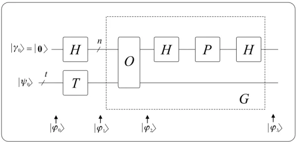
2 stands for the auxiliary qbit required for the proper operation of the algorithm. During the search the algorithm repeats the so-called Grover operatorG depicted in Fig. 3.1 and defined as

G,HP HO, (3.2)

where

O =I−2X

x∈S

|xihx| (3.3)

represents the so-called Oracle which inverts (multiplies with−1) the probability amplitudes of the marked states, where the setS stands for the set of the marked entries. H denotes then-qbit Hadamard gate defined as

H|xi= 1

√2ⁿ X

z∈{0,1}ⁿ

(−1)^xz|zi,

2Entries, which are solutions of the search problem are called marked states according to the literature and the ones which do not lead to a solution are referred to as unmarked ones.

(28)

H P H O

H

n

=

t

T

G

g₀ 0

y₀

j₀ j₁ j2 j3

Fig. 3.1 Circuit implementing the Grover operator

wherexzrefers to the binary scalar product of the twon-bit integer numbers considering them as binary vectors (sum of bitwise products modulo 2). The phase shifter gate P performs a similar operation toOin (3.3) but it flips only the probability amplitude belonging to|0i

P ,(2|0ih0| −I). (3.4)

In order to determine the optimal number of Grover gates, i.e. the least number which minimizes the probability of failed searchP_ε, we introduce a two-dimensional geometrical representation of the search. First we divide the indices into two sets, one (S) for the marked and another (S) for the unmarked ones i.e. we build two superpositions comprising uniformly distributed computational basis states

|αi , 1

√N −M X

x∈S

|xi, (3.5)

|βi , 1

√M X

x∈S

|xi, (3.6)

where|αiand|βiform an orthonormal basis of a two-dimensional Hilbert space as depicted in Fig. 3.2.

Now let us follow the effect of G on |γi in Fig. 3.2. Since the Oracle flips the probability amplitudes of all the marked indices forming |βi, thus because of the Oracle

|γi will be reflected at an axis |αi. The two Hadamard gates H together with P in the middle perform the so-called inversion about the average transformation which is nothing else than a reflection onto|γi. Therefore provided|γiis angular to|αiwith an angle of^Ω₂^γ then the two reflections together produce a single rotation towards|βiby an angle ofΩγ.

(29)

Ö N M - g

3

b g

₁

Ö N Ö M

= G

g

₁

g

₂

= O g

₁

a W

g

W

^g

2 W

g

2 Ö N

Fig. 3.2 Geometrical interpretation of the Grover operator

Sure success search requires in this approach an index register rotated from|γito|βi since a measurement on |βialways provides one of its basis vectors (indices). Thus the number of rotations ensuring absolute success can be easily calculated in the following way

ˆlj =

π

2 +jπ− ^Ω2^γ

Ωγ

, (3.7)

which is minimal ifj = 0. Typicallylopt = ˆl0must be an integer thus Lopt =bˆl0e=

$_π

2 − ^Ω2^γ

Ωγ

'

, (3.8)

whereb·edenotes the rounding function to the nearest integer.

Because of this correctionG^L^opt|γiwill be angular to|βi, hence the measurement may answer with a wrong (unmarked) index. The probability of error can be computed as the squared absolute value of the projection ofG^L^opt|γionto axis|αi

P_ε =hα|G^L^opt|γi= cos²

(2L_opt+ 1)Ω_γ 2

, (3.9)

where the only missing parameterΩ_γcan be obtained as Ωγ = 2 arcsin

rM N

!

. (3.10)

(30)

Combining these results a quite surprising fact can be reached, namelyLopt = Oq

N M

compared to the classical caseO _M^N

.

IfM is not given as an input parameter then phase estimation based quantum counting can be applied with the help of whichM can be found in a computationally efficient way.

In possession of all the required results regarding the basic Grover algorithm. We can now focus our attention on its generalization.

3.2 THE GENERALIZED GROVER ALGORITHM

During the previous analysis of the basic Grover algorithm we aspired to find a suitable trade off between computational complexity (number of rotations or more precisely number of database queriesl) and uncertainty (probability of errorPε). We tried to use as few iterations as possible meanwhile ensuring as high probability of success as achievable. Moreover we have some limitations that may prevent the application of our clever quantum searching algorithm in many practical cases.

• Unfortunately sure success can not be guaranteed merely in exchange of increased number of rotations in the basic Grover algorithm. We have proposed some techniques (e.g. extended database with ’dummy’ entries) a in [82] which provides sure success asymptotically but they requireO(N)rotations to achieve this. However, there are technical problems where we are not permitted to exceed a givenP˘εwhile the number of Grover operators has also to be upperbounded.

• According to the potential applications of Grover’s database search algorithm in practice, larger quantum systems should be taken into account where the input index register of the algorithm is given as an arbitrary output state of a former circuit and the output of the algorithm can feed another circuit without any measurement. Therefore we need a modified Grover algorithm which allows arbitrary initial state instead of the originalH|0i.

In order to tame the above listed problems the original Grover algorithm will be generalized and discussed in the next subsections.

3.2.1 Generalization of the basic Grover database search algorithm

Before investigating the possibilities how to introduce some freedom into the Grover algorithm enabling its generalization let us summarize our knowledge about the Grover operator

G,HP HO, where

P ,2|0ih0| −I,

(31)

O ,I−2X

x∈S

|xihx|.

These definitions were motivated by considerations emerging during the design of the searching algorithm. Furthermore it is known that the Hadamard transform is nothing else than a special QFT. Therefore it seems to be reasonable to replace the original operators with more general ones. New parameters can be involved in this way which could be the base of a more efficient solution.

1. We allow an arbitrary unitary gateU instead of the Hadamard gateH.

2. We let the Oracle to rotate the probability amplitudes of the marked items in the index register with angleφin lieu ofπ(the original setup), whereφ ∈[−π, π]. Thus (3.3) is altered to

O →Iβ ,I+ e^jφ−1 X

x∈S

|xihx|, (3.11) where subscriptβrefers to the fact that the Oracle modifies the probability amplitudes of the computational basis states forming|βi. The matrix ofIβis a modified identity matrix with diagonal elementsIβxx =e^jφ ifx∈S.

3. Analogously to the Oracle above, the controlled phase gate P which was working originally on state|0ishould be based on an arbitrary basis state |ηi resulting in a multiplication bye^jθ instead of−1, whereθ ∈[−π, π]. In more exact mathematical formalism

P →Iη ,I+ e^jθ−1

|ηihη|. (3.12)

The matrix ofI_η is a modified identity matrix with diagonal elementI_β_xx = e^jθ if x=η.

4. Finally the initial state of the index register at the input of the first Grover gate is considered as

|γ1i,

N−1

X

x=0

γ1x|xi, (3.13)

whereP(N−1)

x=0 |γ1x|² = 1as appropriate.

Next the two basis vectors|αi and|βi comprising the indexes leading to unmarked items (setS) and that of ending in a marked entry (setS) should be redefined, which were originally set in (3.5) and (3.6), respectively

|αi= 1 qP

x∈S|γ1x|² X

x∈S

γ1x|xi, (3.14)

|βi= 1 qP

x∈S|γ_1x|² X

x∈S

γ1x|xi. (3.15)

(32)

Observing the new basis vectors |αi and |βi orthogonality is still given between them, hα|βi = 0, since during the pairwise multiplication within the inner product one of the probability aplitudes is always zero.

Remark: In order to avoid the division by zero in (3.14) and (3.15) we require that at least one non-zero probability amplitude exists for the marked and unmarked indices.

If all the entries are marked then we have only vector|βi and a measurement before the search will result in a marked state with certainty. Contrary if the database does not contain the requested item at all then only vector|αiexists. As we will discuss later at the end of Section 3.2.3 both scenarios can be recognized by means of a phase estimation. Therefore in the forthcoming analysis we assume that both vectors exist that is neither of the two sets are empty.

Now it is time to construct the generalized Grover operatorQfrom previously defined gates(G→Q)

Q , −U IηU^†Iβ =−U I + e^jθ−1

|ηihη| U^†Iβ

= − U IU⁻¹+ e^jθ−1

U|ηihη|U^† Iβ

= − I+ e^jθ−1

|µihµ|

I_β, (3.16)

where

|µi,U|ηi (3.17)

and relationU^† =U⁻¹is exploited in consequence of the unitary property.

In possession ofN-dimensionalQfirst we have to prove that its output vector always remains in the2-dimensional space of|αiand|βi, which helps us to preserve our rotation based visualization. This requires the proof of the following theorem:

Theorem 3.1. If the state vectors|αiand|βiare defined according to (3.5) and (3.6) and both of them contain at least one nonzero probability amplitude, as well as the unitary op- eratorU and an arbitrary state|ηiare taken in such a way thatU|ηilies within the vector spaceV spanned by the state vectors|αiand|βi, then the generalized Grover operatorQ preserves this 2-dimensional vector space. In other words for any|vi ∈V,Q|vi ∈V is true.

U|ηi − hβ|U|ηi|βi= q

1− |hβ|U|ηi|²|αi,

(33)

from which|αican be expressed in the nontrivial case i.e. if|hβ|U|ηi| 6= 1as

|αi= 1 q

1− |hβ|U|ηi|²

(U|ηi − hβ|U|ηi|βi). Vector|µiis considered as an arbitrary unit vector inV

|µi2 = cos (Ω)|αi+ sin (Ω)e^jΛ|βi, (3.18) whereΩ,Λ ∈ [−π, π]and the superscript 2refers to the2-dimensional representation of originally N-dimensional |µi. The global phase was omitted in (3.18) since it does not influence the operation and the final result.

In order to reach the well-tried rotation based picture of searching the generalized Grover operator should be determined inV where the required2-dimensional Grover matrix is searched in the form of

Q₂ =

"

Q11 Q12

Q21 Q22

#

. (3.19)

Now we are able to compute the effect ofQ on the basis vectors|αiand |βi. Provided the resulting vectors remain inV then this property will be valid for their arbitrary linear combination (superposition) |vi = a|αi +b|βi because of the superposition principle.

Therefore we applyQfor basis vector|βifirst Q|βi=− I+ e^jθ−1

|µihµ|

Iβ|βi. (3.20)

AsIβ multiplies³every index leading to a marked entry bye^jφ, i.e. |βiis an eigenvector of Iβwith eigenvaluee^jφ thus

Iβ|βi=e^jφ|βi. (3.21)

Substituting (3.21) into (3.20) we get

Q|βi=−e^jφ e^jθ−1

hµ|βi|µi+|βi

. (3.22)

Applying (3.18) and relationhµ|βi=hβ|µi^∗ = sin (Ω)e⁻^jΛ Q|βi = −e^jφ e^jθ−1

sin (Ω)e⁻^jΛ cos (Ω)|αi+ sin (Ω)e^jΛ|βi

−e^jφ|βi

= −e^jφ e^jθ−1

sin (Ω) cos (Ω)e⁻^jΛ

| {z }

Q21

|αi +−e^jφ

e^jθ−1

sin²(Ω) + 1

| {z }

Q22

|βi. (3.23)

Moreover, the other two entries inQcan be determined by feedingQwith|αi Q|αi=− I+ e^jθ−1

|µihµ|

Iβ|αi, (3.24)

3The OracleOdid the same using multiplication factor−1.

(34)

where Iβ|αi = |αi, because only those indices belonging to solutions of the searching problem are rotated byIβ others are left unchanged⁴. Exploiting the relation

hµ|αi=hα|µi^∗ = cos (Ω) (3.25) we get the missing two elements

Q|αi=−

1 + e^jθ−1

cos²(Ω)

| {z }

Q11

|αi+−

e^jθ−1

cos (Ω) sin (Ω)e^jΛ

| {z }

Q12

|βi (3.26)

Based on equations (3.23) and (3.26) we have matrixQ₂ in a suitable2-dimensional form

Q₂ = −

"

1 + e^jθ−1

cos²(Ω) e^jφ e^jθ−1

sin (Ω) cos (Ω)e^jΛ e^jθ−1

cos (Ω) sin (Ω)e⁻^jΛ e^jφ

1 + e^jθ−1

sin²(Ω)

#

= −

"

e^jθcos²(Ω) + sin²(Ω) e^jφe⁻^jΛ e^jθ−1_sin(2Ω)

2

e^jθ−1

e^{jΛ sin(2Ω)}₂ e^jφ

e^jθsin²(Ω) + cos²(Ω)

# .

From this point forwardQalways refers to the2-dimensional Grover matrix, if not indicated otherwise.

3.2.2 Required number of iterations in the generalized Grover algorithm

Having obtained the 2-dimensional generalized Grover operatorQ, we try to follow the rotation based representation of the search. Therefore the optimal number of iterations (Grover gates) ls required to find a marked item with sure success should be derived.

Starting from initial state|γ1isure success can be provided if

hα|Q^l^s|γ₁i= 0, (3.27)

which stands for having an index register orthogonal to the vector including all the indices which do not lead to a solution. Because |αiand |βi are orthogonal and|γ1i ∈ V, this assumption can be interpreted asQ^l^s|γ1iis parallel to|βii.e. Q^l^s|γ1i=e^jδ|βi. In this case sure success can be reached after a single measurement. SinceQis unitary and therefore it is a normal operator too, hence it has a spectral decomposition

Q=q1|ψ1ihψ1|+q2|ψ2ihψ2|, (3.28)

4Thus|αiand1are eigenvector and eigenvalue ofIβrespectively.

(35)

whereq1,2denote the eigenvalues ofQand|ψ1,2istand for the corresponding eigenvectors, respectively. Thus the following equalities hold

Q|ψ1,2i=q1,2|ψ1,2i, (3.29) where hψ1|ψ2i = 0, because of the orthogonality property of the eigenvectors of any normal operators. The eigenvalues which can be determined from the characteristic equation det (Q−qI) = 0are

q_1,2 =−e^j(^θ+φ2 ±Υ). (3.30) In addition we claim the following restriction on angleΥ

cos(Υ) = cos

θ−φ 2

+ sin²(Ω)

cos

θ+φ 2

−cos

θ−φ 2

. (3.31)

In possession of the eigenvalues the next step towards the optimal number of iterations is the determination of the normalized eigenvectors|ψ1,2i, which are

|ψ1i= cos (z)e^j(^φ2−Λ)|αi+ sin (z)|βi, (3.32)

|ψ₂i=−sin (z)e^j(^φ2−Λ)|αi+ cos (z)|βi, (3.33) where

sin²(z) = sin²(2Ω) sin² ^θ₂ 2 1−cos ^θ₂

cos ^φ₂ −Υ

−2 cos (2Ω) sin ^θ₂

sin ^φ₂ −Υ.

The detailed derivation of the eigenvectors and eigenvalues can be found in Appendices 16.1 and 16.2.

Having the required elements of the spectral decomposition ofQin our hand we are able to calculate the operator representing thel-times repetition ofQ

Q^l = q^l₁|ψ1ihψ1|+q₂^l|ψ2ihψ2|= (−1)^le^j^·^l(^θ+φ2 )·

·

"

e^j2(^φ2−Λ) e^jlΥcos²(z) +e⁻^jlΥsin²(z)

jsin (lΥ) sin (2z)e^j(^φ2−Λ) jsin (lΥ) sin (2z)e⁻^j(^φ2−Λ) e^jlΥsin²(z) +e⁻^jlΥcos²(z)

# , (3.34) where we exploited the fact thathψ1|ψ2i = hψ2|ψ1i = 0. Based on (3.34) the optimalls

enabling sure success can be derived using (3.27) which is fulfilled if both – the real and the imaginary – parts ofhα|Q^l^s|γ1iare equal to zero.

Let|γ₁ibe defined as an arbitrary unit vector inV standing for the initial state of the index qregister

|γ1i= cos Ω_γ

2

|αi+ sin Ω_γ

2

e^jΛ^γ|βi. (3.35)

(36)

Thus (3.27) becomes

hα|Q^l^s|γ1i = cos Ωγ

2

Q^l₁₁^s + sin Ωγ

2

e^jΛ^γQ^l₁₂^s =

= cos Ωγ

2

e^jl^s^Υcos²(z) +e⁻^jl^s^Υsin²(z) + + je^j(^φ2−Λ+Λγ) sin (l_sΥ) sin (2z) sin

Ωγ

2

= 0. (3.36)

First we calculate the real part of (3.36)

<

2

cos (lsΥ) cos²(z) + cos (lsΥ) sin²(z)

| {z }

cos(lsΥ)

−

− sin

Λγ−Λ + φ 2

sin (lsΥ) sin (2z) sin Ωγ

2

= cos Ωγ

2

cos (lsΥ)−sin Ωγ

2

sin (lsΥ) sin (2z) sin

Λγ−Λ + φ 2

= 0, (3.37)

which is followed by the imaginary part

=

2

sin (lsΥ) cos²(z)−sin (lsΥ) sin²(z)

| {z }

sin(lsΥ) cos(2z)

+

+ cos

Λγ−Λ +φ 2

sin (lsΥ) sin (2z) sin Ωγ

2

= 0. (3.38) Let us first consider thatsin (lsΥ) = 0⇒cos (lsΥ) = 1. In this case the real part of (3.37) is simplified to

cos Ωγ

2

cos (lsΥ) = cos Ωγ

2

= 0⇒Ωγ = 0±kπ,

while the imaginary part equals constantly 0. Therefore this scenario represents the situation where all the entries are unmarked. Contrary ifsin (lsΥ)6= 0then

=

hα|Q^l^s|γ1i

sin (l_sΥ) = cos

Λγ−Λ +φ 2

sin (2z) sin Ωγ

2

+ cos Ωγ

2

cos (2z) = 0.

(3.39) Equation (3.39) does not depend on ls, which makes it suitable to determine the so called „matching condition” (MC), the relationship betweenθandφ

cos

Λγ−Λ +φ 2

=−cot (2z) cot Ωγ

2

, and thus

tan φ

2

= cos (2Ω) + sin (2Ω)·tan

Ωγ

2

cos (Λ−Λγ) cot ^θ₂

−tan

Ωγ

2

sin (2Ω) sin (Λ−Λγ)

. (3.40)

(37)

It is worth emphasizing that according to (3.31)Υseems to be4πperiodical in function of θ, which implies4π periodicity forφas well when determiningφ formθ becauseΥalso depends onφ. This seems to be inconsistent with the fact that eigenvaluesq1,2 should be 2π periodical in θ andφ, see (3.30). This problem can be resolved ifφ(θ) is calculated for the range[−2π,2π]in function ofθ ∈[−2π,2π]. Practically±2πshould be added to φif it has a cut-off at certain θs. The points whereφ(θ)has cut-offs within the range of [−2π,2π]can be determined easily in the following manner

φ=±π⇒tan φ

2

=±∞.

Since the numerator of the matching condition in (3.40) is constant inθ, hence the denominator has to be zero to achieve the condition φ = ±∞. The cut-off angles θco1,2 can be derived from denominator of (3.40) as follows

cot θ

2

= tan Ωγ

2

sin (2Ω) sin (Λ−Λ_γ) thus the cut-off angles in[−2π,2π]are

θco1 = 2arccot

tan Ω_γ

2

sin (2Ω) sin (Λ−Λγ)

, (3.41)

θco2 = θco1 ±2π. (3.42)

We depictedφ(θ)with and without the±2πcorrection in Fig. 3.3. The cut off points are in this caseθ = ±π. By means of this correction2π periodicity ofΥis achieved, hence the eigenvalues and eigenvectors ofQ, evenQitself can boast a2πperiodicity inθ.

Now, the way is open to determinelsfrom (3.37) supporting a final measurement with Ps = 1. The matching condition (3.40) should also be considered leading to

cos

lsΥ + arcsin

sin φ

2 −Λ + Λγ

sin

Ω_γ 2

= 0, which is equivalent to

lsΥ =±π

2 ±iπ−arcsin

sin φ

2 −Λ + Λγ

sin

Ωγ

2

, (3.43)

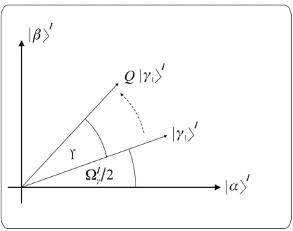
where ±iπ, i > 1 can be omitted from the right hand side, because it would result in a biggerlsthan absolutely necessary. Unlike the basic algorithm wherei >0could result in a more accurate measurement – in exchange of increased number of rotations – in case of the generalized algorithmi= 0,1can providePε= 0. Expression (3.43) can be interpreted in the following way. The generalized Grover operator(Q)rotates the new initial state|γ₁i⁰ having the initial angle

Ω⁰_γ

2 = arcsin

sin φ

2 −Λ + Λγ

sin

Ω_γ 2

(3.44)