Rotation about an arbitrary axis and reflection through an arbitrary plane
Emőd Kovács
Department of Information Technology Eszterházy Károly College
emod@ektf.hu
Submitted April 22, 2012 — Accepted November 7, 2012
Abstract
The aim of this paper is to give a new deduction of Rodrigues’ rotation formula. An other benefit of the this deduction is to give a transforma- tion matrix of reflection through an arbitrary plane with the same deduction method. In our opinion this deduction method is better for students, who are learning computer graphics.
Keywords: Point transformation, Transformation Matrix, Rotation, Reflec- tion, Rodrigues’ rotation formula,
MSC: Primary 68U05, Secondary 65D18
1. Introduction
In the theory of three-dimensional (3D) rotation Rodrigues’ rotation formula (see [7]) is an efficient matrix for rotating an object around arbitrary axis. In this paper we will deduct the matrix form in a different way from the well known method which is published in Rodrigues’ paper [7], cited in Johan’s paper [6] and also described in Wolfram Mathworld site (see [1]). First we give a short introduction of linear point transformation, then we inroduce a new deduction of reflection about an arbitrary axis. Next, we will prove, that our matrix is analogous to the original Rodrigues’
formula. In section three, we describe a matrix of reflection through an arbitrary plane, which is a consequence of our deduction.
http://ami.ektf.hu
175
1.1. Linear Point Transformation
Three dimensional point transformation is one of the well known computer graphics methods, when we manipulate the points of objects, like rotate, translate and scale.
Based on the advantages of homogeneous coordinates, 3D transformations can be represented by 4×4 matrices (see [2] and [3]). Generally the following matrix equation describes the point transformation.
p0 = M·p, (1.1)
x01 x02 x03 x04
=
m11 m12 m13 m14
m21 m22 m23 m24
m31 m32 m33 m34
m41 m42 m43 m44
·
x1
x2
x3
x4
.
When we use more 3D transformations after each other, it is constructed of matrix multiplications (see [8]), therefore composition of 3D transformation can be repre- sented by the multiplication of transformation matrices. The order of multiplication depends on the original form of matrix equation, since the matrix multiplication was noncommutative operation. If we multiply the point from left with the trans- formation matrix in Eq. (1.1), then we must multiply the transformation matrices in reverse order. LetsM1the first,M2 the second transformation matrix, then
p0=M1·p, p00=M2·p0.
Using the associative property it becomes
p00=M2·(M1·p) = (M2·M1)·p.
Therefore we multiply the matrices in reverse orderM3=M2·M1, from that p00=M3·p.
If the point is multiplied by the transformation matrix from the right, then it means the equivalent system. Some graphics library, e.g. DirectX use the latter method, in this case these system use the transposed matrices.
In this paper we deal with the general case of rotation about an arbitrary axis in space. It frequently occurs e. g. in robotics, animation and simulation.
2. Rotation about an arbitrary axis
If we want to construct rotation about an arbitrary axis, then we have a good solu- tion namely Rodrigues’ rotation formula, see [1] on Wolfram MathWorld site. Lots of literatures and internet sources give this method. The problem is that the math- ematical deduction is not suited for the previous section from methodical aspect.
Lots of students could not understand the mathematical deduction of Rodrigues’
formula, which is presented on the Wolfram MathWorld site, and therefore some
of them could not use it. When we teach basic point transformations and we try to extend it towards the composition of 3D transformations, then it could be a good example about the rotation about an arbitrary axis. It would be better if we can give the Rodrigues’ rotation matrix with the composition of basic linear point transformations, and apply multiplication of transformation matrices. In this pa- per we deduce the rotation matrix and prove the computed matrix is an equivalent of the Rodrigues’ formula. Anyone can find the deduction in Rogers’s textbook [8], but now we continue the computation.
The basic idea is to make the arbitrary rotation axis coincide with one of the coordinate axis. Assume an arbitrary axis in space passing through the point P0(x0, y0, z0)andP1(x1, y1, z1).
Figure 1: Rotation about an arbitrary axis
In this case rotation about this axis by some angleθ is accomplished using the following procedure:
1. Translate theP0(x0, y0, z0)axis point to the origin of the coordinate system.
2. Perform appropriate rotations to make the axis of rotation coincident with z-coordinate axis.
3. Rotate about thez-axis by the angleθ.
4. Perform the inverse of the combined rotation transformation.
5. Perform the inverse of the translation.
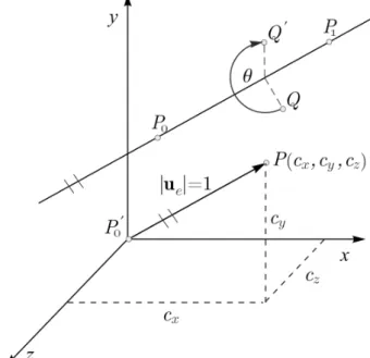
For the simplicity we compute the u=P1−P0 vector, which after the normal- ization can give us the direction cosines of axis:
ue:= u
|u| = (cx, cy, cz).
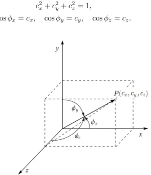
In Fig. 2 the direction cosines are satisfied the following equation:
c2x+c2y+c2z= 1,
cosφx=cx, cosφy =cy, cosφz=cz.
Figure 2: Direction cosines The required translation matrix is
T(−p0) =
1 0 0 −x0
0 1 0 −y0
0 0 1 −z0
0 0 0 1
.
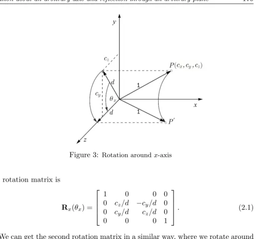
In the next step the procedure requires two successive rotation about thex-axis by the angleθxandy-axis by the angleθy.After the rotation around the thex-axis the original rotation axis will be in the[x, z]coordinate pane. (See Fig. 3).
From the Fig. 3 comes d =q
c2y+c2z, and we do not calculate explicitly the angleθx, because we only use its sin and cosine values in the rotation matrix:
sinθx= cy
d, cosθx= cz
d.
Figure 3: Rotation aroundx-axis
The rotation matrix is
Rx(θx) =
1 0 0 0
0 cz/d −cy/d 0 0 cy/d cz/d 0
0 0 0 1
. (2.1)
We can get the second rotation matrix in a similar way, where we rotate around they-axis by angleθy.
Figure 4: Rotation aroundy-axis
From the Fig. 4 comes
sinθy =d, cosθy =d.
The rotation matrix is with negative direction
Ry(−θy) =
d 0 −cx 0
0 1 0 0
cx 0 d 0
0 0 0 1
. (2.2)
The complete transformation is
M = T−1(−p0)R−x1(θx)R−y1(−θy)Rz(θ)Ry(−θy)Rx(θx)T(−p0), (2.3) where the upper index−1means the inverse transformation, so
M = T(p0)Rx(−θx)Ry(θy)Rz(θ)Ry(−θy)Rx(θx)T(−p0), (2.4) where we used the reverse multiplication order as we mentioned in the previous section. The computation is finished at this point in Rogers’s textbook [8].
Now we are giving one of our new results, and in the section 2.1 we are proving the formulas with Maple computer algebra system.
The formula in (2.3) can be enough, if someone only use the basic transformation matrices in the matrix class of the graphics engine. But methodically for the better understandability and based on our students searching practice in internet literature, we must continue the calculation.
Let multiply the inside five matrices
R=Rx(−θx)Ry(θy)Rz(θ)Ry(−θy)Rx(θx), (2.5) and
M=T(p0)RT(−p0).
Consider that the inverse of rotation matrix equals with the transposed matrix, we get
R=RTx(θx)RTy(−θy)Rz(θ)Ry(−θy)Rx(θx). (2.6) In the next section we are going to prove that if we expand the matrix multipli- cation in Eq. (2.5), then we get the general Rodrigues’ form. In [9] or in [1] we can find the totally different deduction of the Rodrigues’ form, but as we mentioned we are not satisfied the authors deduction way, therefor we give a new solution.
The Maple CAS is very robust and efficient tool for calculating multiplication of transformation matrices.
2.1. Proof with Maple
The main problem of the proof is that multiplication of five matrices in Eq. (2.6).
In order to correct calculation we used Maple computer algebra system (CAS). In [4] and [5] the author explains why Maple is a useful tool for teaching computer graphics in higher education. In Eszterházy Károly College we use CAS software in teaching undergraduate students studiing Software Information Technology bach- elor course.
We can use the power of the linalg package of Maple, to easily multiply the five matrices.
The Maple command is
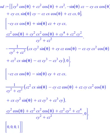
> rod:=simplify(Transpose(RX).Transpose(RY).RZ.RY.RX);
where we used that the transposed rotation matrix equals the inverse of the rotation matrix, and the “rod” means the Rodrigues’ form. After we used the built-insimplify function we got the output in Fig. 5.
Figure 5: First result in Maple
The computed formula is extremely complicated. So we must look for other
simplification possibilities. We can use the combination ofsimplifyandsubstitution functions repeatedly:
for i from 2 to 3 do for j from 2 to 3 do
rod [ i , j ]:= s i m p l i f y ( subs ({ cx^2=1−(cy^2+cz ^2)} , rod [ i , j ] ) ) ; od ;od ;
We can see the output in Fig. 6. Thecollect function was used many times, which
Figure 6: After the simplification collected coefficients. One of them is the following:
rod [ 1 , 1 ] : = c o l l e c t ( rod [ 1 , 1 ] , cos ( theta ) ) ;
After we use thecy2+cz2= 1−cx2equation we get better form. In this paper we do not give the total Maple worksheet. The reader can download it from the following link:
http://aries.ektf.hu/˜emod/mapleporoof.html Finally we got the following result:
cosθ+c2x(1−cosθ) cxcy(1−cosθ)−czsinθ cxcz(1−cosθ) +cysinθ 0 cycx(1−cosθ) +czsinθ cosθ+c2y(1−cosθ) cycz(1−cosθ)−cxsinθ 0 czcx(1−cosθ)−cysinθ czcy(1−cosθ) +cxsinθ cosθ+c2z(1−cosθ) 0
0 0 0 1
.
Obviously the result is analogous with the Rodrigues’ formula in the MathWorld sites. (http://mathworld.wolfram.com/RodriguesRotationFormula.html)
Over 90% of the built-in commands in maple are programmed in Maple’s own Pascal-like programming language. Beside this Maple also give exporting facilities to other programming languages. For example the C command translates the Maple pretty output to ANSI C code. The result was converted to C code in optimized form. When we develop new application, then with the help of “copy paste method”
we can put the code easily into the our C, C++, C# or Java program code. Maple command:
C( rod , optimize ) ; Maple output in C:
t1 = cos ( theta ) ; t2 = −t1 + 0 . 1 e1 ; t3 = cx ∗ cx ; t7 = t2 ∗ cy ∗ cx ; t8 = s i n ( theta ) ; t9 = t8 ∗ cz ; t11 = t2 ∗ cz ; t12 = t11 ∗ cx ; t13 = t8 ∗ cy ; t16 = cy ∗ cy ; t19 = t11 ∗ cy ; t20 = cx ∗ t8 ; t24 = cz ∗ cz ;
cg0 [ 0 ] [ 0 ] = t2 ∗ t3 + t1 ; cg0 [ 0 ] [ 1 ] = t7 − t9 ; cg0 [ 0 ] [ 2 ] = t12 + t13 ; cg0 [ 0 ] [ 3 ] = 0 . 0 e0 ;
cg0 [ 1 ] [ 0 ] = t7 + t9 ; cg0 [ 1 ] [ 1 ] = t2 ∗ t16 + t1 ; cg0 [ 1 ] [ 2 ] = t19 − t20 ; cg0 [ 1 ] [ 3 ] = 0 . 0 e0 ;
cg0 [ 2 ] [ 0 ] = t12 − t13 ; cg0 [ 2 ] [ 1 ] = t19 + t20 ; cg0 [ 2 ] [ 2 ] = t2 ∗ t24 + t1 ; cg0 [ 2 ] [ 3 ] = 0 . 0 e0 ; cg0 [ 3 ] [ 0 ] = 0 . 0 e0 ; cg0 [ 3 ] [ 1 ] = 0 . 0 e0 ; cg0 [ 3 ] [ 2 ] = 0 . 0 e0 ; cg0 [ 3 ] [ 3 ] = 0 . 1 e1 ;
3. Reflection through an arbitrary plane
It is often necessary to reflect an object through an arbitrary plane other than one of the coordinate planes like x= 0, y = 0and z = 0. We can deduct the trans- formation matrix similar to what was described in the previous section. The basic idea is to make the arbitrary reflection plane coincide with one of the coordinate planes. Assuming an arbitrary plane in space is given by three pointsP0(x0, y0, z0), P1(x1, y1, z1)andP2(x2, y2, z2), these points are noncollinear.
According to the previous section one possible procedure is:
1. Translate the reflection plane to the origin of the coordinate system with the help of knownP0(x0, y0, z0)point.
2. Perform appropriate rotations to make the normal vector of the reflection plane at the origin until it coincides with the +z-axis (see Eqs. (2.1) and (2.2)); this makes the reflection plane the z= 0coordinate plane.
3. After that reflect the object through thez= 0 coordinate plane.
4. Perform the inverse of the combined rotation transformation in step 2.
5. Perform the inverse of the translation in step 1.
From the three points of the reflection plane is easy to calculate the normal vector by the crossproduct ofa=P1−P0 andb=P2−P0 vectors:
n=a×b.
For simplicity we normalize the normal vector, which can give us the direction cosines similar to the previous section:
ne : = n
|n| = (cx, cy, cz).
In step 2 the rotation matrices will be the same that were used during the rotation about an arbitrary axis. Finally the seven transformation matrices were multiplied in reverse order:
M=T(p0)Rx(−θx)Ry(θy)R(x,y)ef lectRy(−θy)Rx(θx)T(−p0).
Similar to the previous section we multiply the five inside matrices:
Ref lect=Rx(−θx)Ry(θy)R(x,y)ef lectRy(−θy)Rx(θx), (3.1) then
M=T(p0)Ref lectT(−p0). (3.2)
The general reflection matrix in Eq. (3.1) has no special name in the textbooks.
Similarly to the previous section we use the Maple computer algebraic system to give a simplified form of the transformation matrix:
Ref lect=
1−2cxcx −2cycx −2czcx 0
−2cycx 1−2cycy −2cycz 0
−2czcx −2cycz 1−2czcz 0
0 0 0 1
,
since the inverse of reflection is the same with itselfR−ef lect1 =Ref lect.Good choice to perform the multiplications in Eq. (3.2), because the result is not complicated:
Ref lect=
1−2c2x −2cxcy −2cxcz −2cxd
−2cxcy 1−2c2y −2cycz −2cyd
−2cxcz −2cycz 1−2c2z −2czd
0 0 0 1
, (3.3)
where thed=−cxx0−cyy0−czz0. The previous matrix is a good result from the methodological aspect, because the student also can find the similar version in the D3DXMatrixReflect function of DirectX:
P =normalize(P lane);
−2∗P.a∗P.a+ 1 −2∗P.b∗P.a −2∗P.c∗P.a 0
−2∗P.a∗P.b −2∗P.b∗P.b+ 1 −2∗P.c∗P.b 0
−2∗P.a∗P.c −2∗P.b∗P.c −2∗P.c∗P.c+ 1 0
−2∗P.a∗P.d −2∗P.b∗P.d −2∗P.c∗P.d 1
,
where the matrix equals the matrix in Eq. (3.3) after transposition. The normalize(P lane) function normalizes the normal vector of the plane. P.a, P.b andP.care the coefficients in the plane equation, and obviously the coordinates of normalized normal vector as well (see [10]):
P.a∗x+P.b∗y+P.c∗z+P.d= 0,
andP.dcontains the one pointP(x0, y0, z0)of the plane as we mentioned above:
P.d=−P.a∗x0−P.b∗y0−P.c∗z0,
moreoverP.d comes from the dot product of the normal vector and P (see [10]).
If our student use the deduction in the section 3, then the D3DXMatrixReflect DirectX function becomes understandable without difficulties.
4. Conclusion
In this paper we proposed a better deduction of Rodrigues’ rotation formula than you can find in a lots of literature (e.g see [1]). In other text book you can find the similar deduction to our method (see [8]), but in this paper we continued the deduction and demonstrate the equality between the result and the Rodrigues’
form. From the aspect of teaching computer graphics in higher education, our method is better understandable for the students. Moreover, our deduction comes naturally from the composition of 3D transformations. An additional benefit is that our method is a good solution to deduct transformation matrix of reflection through an arbitrary plane.
References
[1] Belongie, S., Rodrigues’ Rotation Formula, From MathWorld –A Wolfram Web Resource, created by Eric W. Weisstein.
http://mathworld.wolfram.com/RodriguesRotationFormula.html
[2] Foley, J., van Dam, A.,Feiner, S., Hughes, J., Computer Graphics Principles and Practice, Addison-Wesley, 1996.
[3] Juhász, I.,Számítógépi grafika és geometria, Miskolci Egyetemi Kiadó, 1993.
[4] Kovács, E., Using some mathematical program in computer graphics teaching, 7th ICECGDG Cracow. International Conference on Engineering Computer Graphics and Descriptive Geometry July 18–22. 1996. Conference Proceedings Volume 2 p.
546–549.
[5] Kovács, E., Using Maple in teaching of computer graphics, International Conference on Applied Informatics, Eger 1995. Conference Proceedings, p. 83–92.
[6] Mebius, J. E., Derivation of the Euler-Rodrigues formula for three-dimensional rotations from the general formula for four-dimensional rotations., arXiv General Mathematics 2007.http://arxiv.org/abs/math/0701759
[7] Rodrigues, O., Des lois géométriques qui régissent les déplacements d’un systéme solide dans l’espace, et de la variation des coordonnées provenant de ces déplace- ments considérés indépendamment des causes qui peuvent les produire. Journal de Mathématiques 5, 1840, 380–440.
[8] Rogers, D. F., Adams, J. A., Mathematical elements for computer graphics, Second Edition, McGraw-Hill publishing Company, 1990.
[9] Watt, A., Policarpo, F., 3D Games: Real-Time Rendering and Software Tech- nology, New York : ACM Press, 2001.
[10] Weisstein, Eric W., From MathWorld – A Wolfram Web Resource http://mathworld.wolfram.com/Plane.html