High Level Technical Drawing

(1)

High Level Technical Drawing

(2)

2

High Level Technical Drawing

Zsolt Tiba

TERC Kft. • Budapest, 2013

(3)

3

End of manuscript / Kézirat lezárva: 2011. szeptember

Reviewer / Lektor: John Graham BEng Mechanical Engineering

ISBN 978-963-9968-67-7

Published by TERC Ltd / Kiadja a TERC Kereskedelmi és Szolgáltató Kft. Szakkönyvkiadó Üzletága, az 1795-ben alapított Magyar Könyvkiadók és Könyvterjesztők Egyesülésének

a tagja

A kiadásért felel: a kft. ügyvezető igazgatója Felelős szerkesztő: Lévai-Kanyó Judit

Műszaki szerkesztő: TERC Kft.

Terjedelem: 7,75 szerzői ív

(4)

4

Figures: János Dulovits, János Juhász, Dániel Tóth

(5)

5

ABBREVIATIONS OF TERMS AND MARKS

turning developed

R radius m

Ø diameter m

flat taper %

conical taper %

sphere R sphere radius m

square

straightness

flatness roundness

circularity

profile of surface

profile of line

angularity

perpendicularity parallelism

symmetry

position concentricity

runout

total runout

A area, cross-section m²

AS actual size m

AD actual deviation µm

BC big clearance µm

BI big interference µm

BL base line

BS basic size m

E modulus of elasticity N/m²

ES upper deviation (hole) µm

EI lower deviation (hole) µm

es upper deviation (shaft) µm

ei lower deviation (shaft) µm

F force, load N

i unit tolerance µm

I unit tolerance µm

IT international tolerance grade

l length m

LD lower deviation µm

LL low limit µm

m mass kg

MC mean clearance µm

MD mean deviation µm

MI mean interference µm

MS mean size m

n speed 1/min

(9)

9 q factor of IT grade

R_eH yield strength N/mm²

R_m tensile strength N/mm²

R_p0.2 yield strength N/mm²

SC small clearance µm

SI small interference µm

T tolerance µm

T_i resultant tolerance µm

t₁ degree of accuracy: fine t₂ degree of accuracy: medium t₃ degree of accuracy: coarse t4 degree of accuracy: very coarse Ra surface roughness average µm Rz peak to valley height average µm

UD upper deviation µm

UL upper limit µm



strength N/mm²



elastic elongation or compression, strain %

(10)

10

LIST OF TABLES

Table 1.1 Preferred sizes of drawings ... 16

Table 1.2 Line thickness groups ... 17

Table 1.3 Recommended heights of letters ... 20

Table 3.1 Conventional representation of materials ... 26

Table 13.1 The values of q factor ... 87

Table 13.2 Tolerance values ... 88

Table 13.3 Fundamental deviations for shafts ... 89

Table 13.4 Fundamental deviations for shafts ... 90

Table 13.5 Fundamental deviations for holes ... 91

Table 13.6 Fundamental deviations for holes ... 92

Table 13.7 Alternatives of free dimension tolerances ... 93

Table 13.8 Preferred fits ... 96

Table 13.9 Form and position tolerance symbols ... 101

Table 14.1 Required average surface roughness ... 108

Table 14.2 Required tolerance grades... 109

Table 14.3 General guidelines for feasible roughness Ra for different processing methods ... 110

Table 14.4 Meaning of surface roughness symbols ... 111

Table 14.5 Symbols specifying the direction of lay... 112

Table 15.1 Rockwell test methods ... 117

Table 15.2. Comparison of the hardness ranges ... 118

Table 15.3 Correlation between hardness and strength ... 119

(11)

11

LIST OF FIGURES

Figure 1.1 Sheet formats ... 16

Figure 1.2 Title block ... 17

Figure 1.3 Principal types of lines ... 18

Figure 1.4 Applying different types of line ... 18

Figure 1.5. Constructing transition lines ... 19

Figure 1.6. Drawing transition lines ... 19

Figure 1.7. Spacing different types of lines ... 19

Figure 1.8 Vertical and inclined lettering ... 20

Figure 2.1. Defining principal views ... 22

Figure 3.1 Indicating views and cutting planes ... 24

Figure 3.2 Drawing auxiliary view ... 25

Figure 3.3 Drawing local view... 25

Figure 3.4 Arranging auxiliary views ... 25

Figure 3.5 Drawing breaking ... 25

Figure 3.6 Applying breaking ... 25

Figure 3.7 Hatching adjacent components ... 26

Figure 3.8 Drawing sectional view ... 27

Figure 3.9 Marking cutting planes ... 27

Figure 3.10 Drawing half-sectional view ... 28

Figure 3.11 Drawing broken-out section ... 28

Figure 3.12 Drawing removed element ... 28

Figure 3.13 Drawing removed section by indicating the cutting plane ... 29

Figure 3.14 Drawing removed section turned by marking the cutting plane ... 29

Figure 3.15 Drawing removed sections ... 29

Figure 3.16 Drawing removed section indicated by its centre line ... 30

Figure 3.17 Drawing removed section by marking the cutting plane ... 30

Figure 3.18 Removed section applying broken out ... 30

Figure 3.19 Removed section revolved into the drawing plane ... 30

Figure 3.20 Drawing offset section ... 31

Figure 3.21 Drawing revolved offset section ... 31

Figure 3.22 Drawing revolved offset section ... 31

Figure 3.23 Drawing revolved section ... 32

Figure 3.24 Drawing developed view ... 32

Figure 3.25 Sectioning curved shape part ... 33

Figure 3.26 Drawing developed section... 33

Figure 3.27 Applying broken out section on half views ... 33

Figure 3.28 Applying broken out section when grazing a surface ... 34

Figure 3.29 Avoiding hatching webs ... 34

Figure 3.30 Breaking out webs ... 35

Figure 3.31 Sectioning a flange ... 35

Figure 3.32 Sectioning a flywheel ... 35

Figure 3.33 Drawing transition lines ... 35

Figure 3.34 Avoiding drawing transition lines ... 35

Figure 3.35 Indicating surface texture ... 36

Figure 3.36 Indicating terminal position ... 36

Figure 4.1 Main types of dimensioning ... 38

Figure 4.2 Indicating coated surfaces ... 38

Figure 4.3 Chain dimensioning and informative dimensioning ... 39

Figure 4.4 Arrowhead ... 39

Figure 4.5 Methods of indicating dimensions ... 39

Figure 4.6 Arrangement of dimensioning ... 39

Figure 4.7 Dimensioning half sectioned view ... 40

Figure 4.8 Dimensioning equiangular features ... 40

Figure 4.9 Dimensioning equidistant features ... 40

(12)

12

Figure 4.10 Dimensioning bolt circle and holes on it ... 40

Figure 4.11 Shape identification symbol, square ... 41

Figure 4.12 Shape identification symbol, sphere ... 41

Figure 4.13 Dimensioning chamfers ... 41

Figure 4.14 Simplified chamfer dimensioning ... 41

Figure 4.15 Oblique dimensioning ... 41

Figure 4.16 Angular dimensioning ... 41

Figure 4.17 Dimensioning non-circular curve ... 42

Figure 4.18 Simplified dimensioning of non-circular curve ... 42

Figure 4.19 Dimensioning non-parallel surfaces ... 42

Figure 4.20 Simplified parallel dimensioning ... 42

Figure 4.21 Simplified parallel angular dimensioning ... 42

Figure 4.22 Co-ordinate dimensioning ... 43

Figure 4.23 Choosing a significant surface as a reference surface ... 44

Figure 4.24 Choosing boundary lines as reference surfaces ... 44

Figure 4.25 Choosing several boundary lines as reference surfaces ... 45

Figure 4.26 Grouping the dimensions ... 45

Figure 4.27 Choosing a common position surface as reference surface ... 45

Figure 4.28 Dimensioning mating elements ... 46

Figure 4.29 Conventional dimensioning of bore-hole ... 46

Figure 4.30 Conventional dimensioning of threaded bore-hole ... 46

Figure 4.31 Conventional dimensioning of threaded blind bore-hole ... 47

Figure 4.32 Conventional dimensioning of bore-hole and threaded bore-hole with counterbore ... 47

Figure 4.33 Conventional dimensioning of threaded bore-hole groups ... 47

Figure 4.34 Dimensioning a shape rolled component ... 48

Figure 4.35 Dimensioning a sheet component ... 48

Figure 4.36 Conical taper ... 48

Figure 4.37 Flat taper ... 48

Figure 4.38 Dimensioning conical taper ... 49

Figure 4.39 Dimensioning flat taper ... 49

Figure 4.40 Showing the taper by dimensions and angle ... 49

Figure 4.41 Giving of measuring place of tapered part ... 49

Figure 4.42 Giving informative dimension signed by mark ... 50

Figure 5.1 Conventional presentation of external threads ... 52

Figure 5.2 Conventional presentation of internal threads ... 52

Figure 5.3 Presentation of threads in section ... 52

Figure 5.4 Ignoring the presentation of the chamfer ... 52

Figure 5.5 Presenting the chamfer of the thread ... 53

Figure 5.6 Drawing intersecting threaded holes in section ... 53

Figure 5.7 Dimensioning a thread profile... 53

Figure 5.8 Dimensioning a thread profile in on a removed element ... 53

Figure 5.9 Drawing a connecting male and female thread in section ... 53

Figure 5.10 Drawing a connecting male and female thread in section having a keyway . 53 Figure 5.11 Drawing a tapered male thread ... 54

Figure 5.12 Drawing a tapered female thread ... 54

Figure 5.13 Different types of screws ... 54

Figure 5.14 Representing locking devices ... 54

Figure 5.15 Representing left-hand threaded screw ... 55

Figure 6.1 Defining common machine element shapes ... 56

Figure 7.1 Drawing a helical spring in view and in section ... 58

Figure 7.2 Ignoring drawing spring coils with centre lines ... 58

Figure 7.3 Drawing ignored spring coils with thin continuous lines ... 58

Figure 7.4 Symbolic presentation of a cylindrical helical spring ... 58

Figure 7.5 Presentation of a conical helical spring in view, in section and symbolic ... 58

Figure 7.6 Presenting a helical extension spring ... 59

Figure 7.7 Presenting a turning helical spring ... 59

(13)

13

Figure 7.8 Representing a buffer spring ... 59

Figure 7.9 Representing an annular spring ... 60

Figure 7.10 Presenting a belleville spring in view, in section and symbolic ... 60

Figure 7.11 Simplified and symbolic presentation of multi-leaf spring ... 60

Figure 7.12 Drawing with load diagram ... 61

Figure 8.1 Bolted joint ... 63

Figure 8.2 Studded joint ... 63

Figure 8.3 Screw fastening ... 63

Figure 8.4 Left-hand bolt and nut ... 63

Figure 8.5 Rivet head shapes ... 63

Figure 8.6 Lap rivet joint ... 64

Figure 8.7 Single strap butt rivet joint ... 64

Figure 8.8 Butt joints ... 64

Figure 8.9 Lap joint ... 64

Figure 8.10 T joint ... 64

Figure 8.11 Corner joint ... 64

Figure 8.12 Presenting a welding joint in section and in view ... 65

Figure 8.13 Simplified presentation of a welding joint ... 65

Figure 8.14 Welding symbols ... 66

Figure 8.15 Placing welding symbols ... 67

Figure 8.16 Dimensioning single V-butt, single Y-butt and double V-butt joints... 68

Figure 8.17 Presenting symmetric intermittent welding ... 68

Figure 8.18 Presenting offset intermittent welding ... 68

Figure 8.19 Additional welding symbols ... 69

Figure 9.1 Presenting saddle keys ... 70

Figure 9.2 Presenting a parallel keyed joint ... 71

Figure 9.3 Presenting a Woodruff keyed joint ... 72

Figure 10.1 Presenting a splined shaft and hub in axonometric projection ... 73

Figure 10.2 Drawing a splined shaft ... 74

Figure 10.3 Drawing a hollow splined shaft in section ... 74

Figure 10.4 Drawing a broken-out section of a splined shaft ... 74

Figure 10.5 Presenting the spline run-out of the shaft ... 74

Figure 10.6 Drawing a splined hub in view and in section ... 75

Figure 10.7 Drawing a splined joint in view and in section ... 75

Figure 11.1 Presenting part of a gear tooth in axonometric projection ... 77

Figure 11.2 Drawing a spur gear ... 78

Figure 11.3 Drawing rack circle on view, in section and in axonometric view ... 78

Figure 11.4 Drawing rack ... 78

Figure 11.5 Presenting anchor wheel ... 79

Figure 11.6 Presenting worm-wheel ... 79

Figure 11.7 Presenting a bevel gear ... 79

Figure 11.8 Drawing meshing spur gears ... 80

Figure 11.9 Drawing a meshing rack and rack circle ... 80

Figure 11.10 Drawing meshing bevel gears ... 80

Figure 11.11 Drawing a meshing worm and worm-wheel ... 81

Figure 11.12 Drawing a sprocket ... 81

Figure 11.13 Drawing a chain drive ... 81

Figure 12.1 Drawing a single grooved ball bearing ... 82

Figure 12.2 Self aligning ball bearing ... 83

Figure 12.3 Single row angular contact ball bearing ... 83

Figure 12.4 Double row angular contact ball bearing ... 83

Figure 12.5 Double row self aligning roller bearing ... 83

Figure 12.6 Single row cylindrical roller bearing ... 83

Figure 12.7 Needle-roller bearing ... 83

Figure 12.8 Tapered roller bearing ... 83

Figure 12.9 Single row ball thrust bearing ... 83

Figure 12.10 Double row ball thrust bearing ... 83

(14)

14

Figure 12.11 Self aligning roller thrust bearing ... 83

Figure 13.1 Defining the sizes ... 85

Figure 13.2 Basic deviations for shafts ... 86

Figure 13.3 Basic deviations for holes... 87

Figure 13.4 Presenting the clearance and interference fit ... 94

Figure 13.5 Dimensions of clearance and interference fits ... 95

Figure 13.6 Dimensions of a transition fit ... 95

Figure 13.7 Nature of fit ... 95

Figure 13.8 Resultant tolerance of the fit ... 96

Figure 13.9–Figure 13.14 Examples for giving limit tolerances ... 99

Figure 13.15–Figure 13.18 Examples for giving ISO tolerances ... 100

Figure 13.19–Figure 13.26 Examples for giving form tolerances ... 103

Figure 13.27–Figure 13.41 Examples for giving position tolerances ... 105

Figure 14.1 The micro-irregularities of the surface ... 106

Figure 14.2 Defining the mean Peak-to-Valley Height ... 107

Figure 14.3 Surface roughness symbols ... 111

Figure 14.4 Giving average surface roughness and peak to valley height ... 113

Figure 14.5 Placement of the surface roughness symbol ... 113

Figure 14.6 Placement of the general average surface roughness symbol ... 113

Figure 14.7 Examples for giving average surface roughness ... 113

Figure 14.8 Giving average surface roughness on the-pitch circle ... 114

Figure 14.9 Giving average surface roughness on the root-line ... 114

Figure 14.10 Giving surface roughness of the thread profile ... 114

Figure 14.11 Giving surface roughness of a coated surface ... 114

Figure 14.12 Giving different surface roughness of the same surface ... 114

Figure 15.1 Standardized tension test specimen ... 115

Figure 15.2 Stress-strain diagram obtained from the standard tensile test ... 116

(15)

15

Objective

A drawing is a graphic presentation of an object, or a part of one, and is the result of the creative thinking of an engineer or technician. All machines and their parts can be presented in the form of a technical drawing and manufactured accordingly. Designing a machine part involves making sketches and technical drawings, and performing the appropriate calculations. Sometimes several alternative designs are presented in drawings, and the best one is selected for the purpose.

Machine drawing is a special “language” of engineers; it is a way of transmitting information as a graphical representation. It allows us to represent machine elements in a simplified and standardised way and to study the constructional build-up of machinery.

Machine drawing enables us to transmit all the information, which is crucial for the process of manufacturing, assembling and understanding the construction. Knowing and applying the standardized methods of presentation is necessary for the machine drawing to be understandable for everyone.

The purpose of writing and composing a book on High Level Technical Drawing is to introduce notions and presentation methods according to the Hungarian Standards.

Furthermore, it makes it possible to acquire the technical terms in connection with the given topic since it is a basic requirement for an engineer to be able to communicate with foreign engineers in English.

(16)

16

1. DRAWING STANDARDS

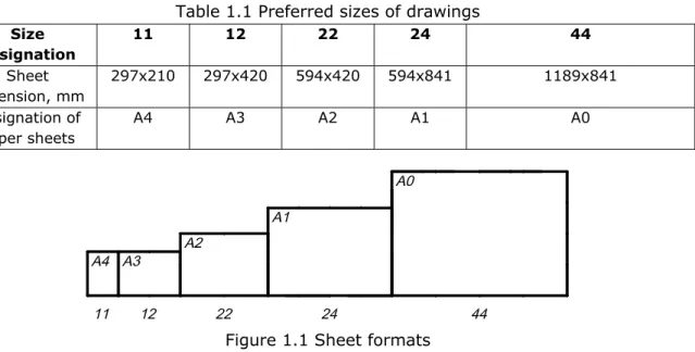
The engineering drawings are made on sheets of strictly defined sizes that are set forth in the Standard (MSZ ISO 5475). The use of standard sizes ensures convenient storage of drawings. The standard establishes five preferred sizes for drawings as tabulated in Table 1.1.

Table 1.1 Preferred sizes of drawings Size

designation

11 12 22 24 44

Sheet dimension, mm

297x210 297x420 594x420 594x841 1189x841 Designation of

paper sheets

A4 A3 A2 A1 A0

Figure 1.1 Sheet formats

Drawing size is designated by two figures in this case: the first indicates how many times one side of the drawing is longer than 297 mm, the second how many times the other side is longer than 210 mm. The basic size for drawings is S11 measuring 297 mm by 210 mm. All other sizes comprise several S11. Thus, S12 is made up of two S11 with adjoining long sides (Fig.1.1).

Depending on the form of the component other drawing sizes are applicable in order to utilize the paper sheet. Hence, in addition to the above preferred sizes, the standard provides for other sizes, which are also comprised of a whole number of S11.

(E.g.: the designation of the sheet dimension of 297x630 is S13.)

(17)

17

1.1 Title blocks

The title block of a drawing is located in the bottom right-hand corner of the sheet. The title block should be arranged along the short side of the sheet in the case of A4 and along the long side of the sheet in all other sizes. Sheets which are smaller than A1 can be used in the standing position with the title block located in this case along the short side too. Sizes and content of title blocks are standardised (DIN 323; MSZ 1700).

The title block may be changed somewhat to suit special requirements of different enterprises. The spaces of the title block are intended for; the name of the (assembly) drawing, name of enterprise or educational institution, description or title of drawing, dates and signatures, name of the definite part (e.g. "casing"), designation of the given drawing, quantity, material, weight, scale, etc. (Fig. 1.2).

Figure 1.2 Title block

In engineering drawing the standard (DIN 15; MSZ ISO 128) specifies different line thickness groups and assigns the thickness of the thick, thin and the medium thickness lines to the given thickness group (Table 1.2). Line thickness depends on the dimension of the part and the complexity, size and purpose of the drawing. In common circumstances thickness group 3a is recommended, namely thick line is 0.7 mm, medium line is 0.5 mm and thin line is 0.25 mm.

Table 1.2 Line thickness groups Lines Line thickness groups

Desig- nation

Thickness 1 2 3 4 5

a b a b a b a b a b a b

Thick s 0.35 0.5 0.7 1.0 1.0 Medium s/2 2s/3 0.18 0.25 0.25 0.35 0.35 0.5 0.5 0.7 0.7 1.0 Thin s/3 s/2 0.13 0.18 0.18 0.25 0.25 0.35 0.35 0.5 0.5 0.7 Display 2s 0.7 1.0 1.4 2.0 2.0

The standard specifies various types of lines as well to enable distinction between the lines pertaining to different surfaces.

(18)

18

Figure 1.3 Principal types of lines

Figure 1.4 Applying different types of line

There are four principal types of lines: continuous (thick, thin and wavy); short-dash;

dot-and-dash or chain (thick and thin) (see Fig. 1.3). Typical applications of the above listed types of lines are shown in Fig. 1.4.

Thick continuous lines are used for:

– drawing visible outlines which are 0.7 mm (thickness group 3a). The chosen thickness group has to be equal for all views in a given drawing representation.

Thin continuous lines used for:

– extension and dimension lines which are 0.25 mm

– hatching in sections, the hatching lines are spaced at 2 to 10 mm depending on the area to be cross-hatched

– transition lines between surfaces, gradually merging into each other as in Fig. 1.5 (a and b lines) and 1.6.

Thin wavy lines used for:

– breaks drawn by a free-hand wavy line Short-dash lines are used for:

– hidden outlines and hidden intersections; the length of a dash ranges from 2 to 8 mm, it is medium thickness (0.35 mm), the spacing between dashes (a) is between 1/2 and 1/4 of their length (see Fig. 1.7).

Thin double-dot-dash lines with long dashes (or long chain lines) are used for:

– axes and centre lines with a thin line (0.25 mm) with dashes approximately 9 mm long spaced at about 3 mm (a1), see Fig. 1.7. Centre of circles should be marked

(19)

19

by two intersecting dashes. For circles of diameters smaller than 12 mm the centre lines are usually drawn with thin continuous lines.

Thin dot-and-dash lines with two dots are used to show:

– a surface smoothly merging into another line indicating bending edge. In this case m2=m1 and a2=a1.

Figure 1.5 Constructing transition lines

Figure 1.6 Drawing transition

lines Figure 1.7 Spacing different types of lines Drawing instruments

There are several computer programs e.g. AutoCAD that make it possible to produce technical drawing in 2 or 3D and that can be saved as a file, and modified and reconstructed without having to draw it again. The aim of attending the Technical Drawing course is to acquire the methods and rules of the simplified and standardized graphical representations of machine elements, components and machine parts and machines. The only way of learning and practicing the fundamental construction principles is to draw by hand.

Accordingly, in a Technical Drawing course the following instruments are used:

 Drawing board: with drawing paper on it, on which a drawing is made.

 Triangles: two types of triangles are used for drawing: 45ô -45ô, 60ô-30ô.

 T-square: consists of two parts, a long ruler and a crosspiece.

 Ruler, French curve, protractor, compass, pencil.

1.2 Lettering

The styles of letters and numbers used for engineering drawings are also standardized (DIN 6776; MSZ ISO 3098) (forms and slant of the capital and lowercase letters). Since all mechanical parts are manufactured according to drawings and all information is given by lettering, it has to be made very carefully.

Table 1.3 indicates the recommended heights of letters and numbers, and their line thickness. The following sizes of characters are recommended: 2.5, 3.5, 5, 7, 10, 14 and 20 mm. The size is determined by the height h (in mm) of capital letters. The letters and numbers have an inclination of 75° to the horizontal. In certain cases drawings may be lettered in vertical characters. The shape of the letters and numbers of medium width are shown in the Fig. 1.8.

(20)

20

Table 1.3 Recommended heights of letters Specification Designation Size groups Height of

capital letters

h 2.5 3.5 5 7 10 14 20

Height of lower-case

letter

5h/7 1.75 2.5 3.5 5 7 10 14

Line thickness h/7 0.3 0.5 0.7 1 1.5 2 3

Minimum line spacing

10h/7 3.5 5 7 10 14 20 28

Reduced line thickness

h/10 0.2 0.3 0.5 0.7 1 1.5 2

Figure 1.8 Vertical and inclined lettering

In machine drawing the 2.5 mm height capital letter is used for tolerances, the 3.5 mm height is used for dimensions, the 5 mm height is used for notice, the 7 mm is used for displaying notice and the 10 mm height is used for item number.

(21)

21

2. TECHNICAL DRAWING

When designing either machines or a component, the first action is often to make freehand pictorial views of the machine or its parts. This process is called technical sketching.

The aim of the technical drawing course is to acquire the methods of sketching machine parts and making and reading the working and assembly drawings. When designing a machine or construction, the following drawings are elaborated:

Schematic representation: a simplified illustration of the machine or of a system, replacing all the elements, by their respective conventional representations.

– Technical sketching: freehand pictorial views of machine or machine parts to render their shape and function.

– Assembly drawing: a drawing that shows the various parts of a machine in their correct working locations. It should furnish the overall dimensions, the linkage dimensions and the dimensions important in terms of operation.

– Shop drawing: pertaining to machine parts or components. It is presented through a number of orthographic views, so that the size and shape of the component is fully understood. It furnishes all the dimensions, tolerances and special finishing processes such as heat treatment, honing, lapping, surface finish, etc.

2.1 Presentation methods in technical drawing

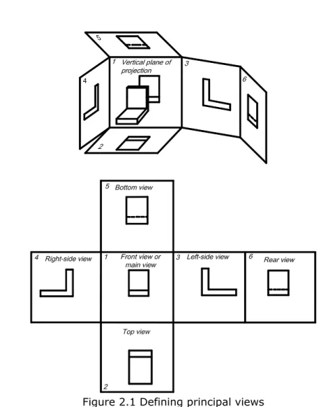
We can imagine an object that is located inside a box and projected orthographically to the corresponding plane of projection. It results in six views that can exist, when all the planes of projection are brought into alignment (see Fig. 2.1).

When drawing a machine part the main view should be selected with respect to its working position (if possible) to reveal its shape and dimensions. Such parts as axles, shafts, bushes, sleeves, tubes, etc., are usually presented in the main view with the axis in the horizontal position, and not necessarily in the working position.

There are several types of views and sections that can reveal the details of a part instead of applying the bottom view, or left hand view and so on, (see chapter 3). The number of applied views and sectional views depends on the complexity of the part and the resources of the drawer. The number of views in an orthographic drawing must be as few as possible but sufficient to provide enough information on the shape and dimensions of the object.

(22)

22 2.1.1 Views

In technical drawings orthographic projection is used in conformity with the standards (DIN 5; MSZ 1701) when constructing views and various sections. The projection of the visible portion of the surface of an object facing the viewer is called a view.

The six views obtained of the above mentioned planes of projection are called:

1 front or main view 2 top view

3 left side view 4 right side view

5 bottom view 6 rear view

Figure 2.1 Defining principal views

The views are not indicated if they are located appropriately relating to the main view, as stipulated by the above mentioned standard. In this case views have to always be in horizontal or vertical alignment with the other views and the projection of one view to another cannot be questioned.

4

(23)

23

3. MACHINE DRAWING

3.1. Presentation methods in machine drawing

Parts are manufactured and assembled according to drawings. A drawing must contain information concerning the shape of the object, its function, dimension, material, surface finish, heat treatment and more.

When making machine drawings the views can be arranged in a specific way. Some views may be located without orthographic connection to the main view or may be incomplete in which case they are bounded by a break line or an axis of symmetry. In this case the direction of viewing is indicated by an arrow designated by the corresponding letter. For indicating the direction of views and cutting planes (see later) capital letters are used.

(24)

24

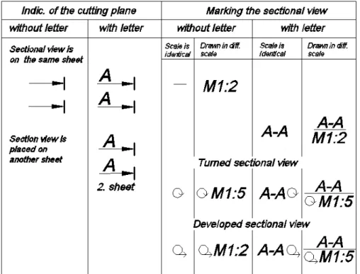
Figure 3.1 Indicating views and cutting planes

The identification of the view and the sectional view is done by using the same letters placed above or close to the view or the sectional view. If the view or sectional view is drawn in a different scale or on another sheet or it is placed in a special way, it must be indicated according to the standard (MSZ ISO 128) as in Fig. 3.1.

Besides the above considered views, machine drawings sometimes use auxiliary views facing arrows. They are resorted to when none of the six principal planes of projection gives the true shape and dimensions of a certain machine part or its elements. Therefore, any surface that is not in line with one of the three major axes needs its own projection plane which must be parallel to the object surface to show the features correctly.

3.1.1 Auxiliary view

When drawing auxiliary views distorted portions of a part are usually not shown. To avoid it the view is broken and bounded by a break line. Examples of arranging auxiliary views are given in Figs. 3.2 (a bracket) and Fig. 3.4. To avoid constructing several ellipses on the horizontal projection, the orthographic drawing should be represented as in Fig. 3.2 with the upper portion projected on an auxiliary plane of projection. Auxiliary views (say, the view facing arrow or facing arrow A) must be accompanied by the corresponding inscriptions, for instance, A, and the appropriate projection of the part must be supplied with an arrow indicating the direction of viewing (see Fig. 3.4).

(25)

25

Figure 3.2 Drawing auxiliary view Figure 3.3 Drawing local view

When arranging views, auxiliary views may be turned through any desired angle for lucidity. In this case the mark of turning should be added, which is placed next to the marking of A, as in Fig. 3.4.

Figure 3.4 Arranging auxiliary views 3.1.2 Local view

Sometimes it is necessary to show only a certain part of the surface of a machine part.

In this case it is expedient to draw only this particular part of the area which is called a local view instead of drawing all the whole orthographic views. The local view boundary is shown by a break line (as in Fig. 3.3). A local view, like an auxiliary one, may be accompanied by an inscription indicating the place where it pertains to. In simple drawing if the origin of the auxiliary view or local view is obvious the designation of the view can be omitted as in Fig. 3.2 and in Fig. 3.3.

3.1.3 Breaking

Breaking may be used to shorten certain views of long parts having similar cross sections throughout the length as in Fig. 3.5. If a view has a break, the dimension line must be drawn without breaks, and the dimension indicates the true length of the part. Fig. 3.6 illustrates a break of a part with cross sections varying in height.

Figure 3.5 Drawing breaking Figure 3.6 Applying breaking

(26)

26

3.2 Sectional views and sections

The rules of making sections are standardised (DIN 6; MSZ ISO 128). If a machine part or an element of which is cut along a plane, then a plane figure is obtained on the cutting plane. This figure is called a section. A sectional view is a view seen when a portion of the object nearest the observer is imagined to be removed by means of a cutting plane or planes, thus revealing the interior construction. However the other views are not affected in any way and always present the entire object. Some distorted elements behind the cutting plane may be omitted for simplification. The section is cross-hatched with thin lines having an inclination angle of 45°.

In assembly drawing the adjacent components should be outlined in different ways by cross-hatching in opposite directions (Fig. 3.7).

Figure 3.7 Hatching adjacent components

If a part is so shaped that 45^o degree sectioning runs parallel or nearly parallel to an outline or an axis, a hatching of 30° or 60° should be used.

The spacing between the hatching lines is estimated by eye but should be uniform. This spacing is usually between 2 and 10 mm depending on the hatched area. Small areas may be section lined at 1.5 mm. Long and narrow sections (less than 2 mm wide) may be made solid black independent of the material. In machine drawing the kind of material has to be indicated by using a specific type of section lining. The conventional symbols for various materials are shown in Table 3.1.

Table 3.1 Conventional representation of materials

Metals Filled up ground

Non-metallic material except those specified below

Electrical winding

Wood cross grain Grindstone

Wood with grain Glass and other

transparent materials Sandwich structure Blade pack

Plain concrete Earth at edges of foundations

Depending on the number of cutting planes, sectional views are classified as follows:

simple (with one cutting plane) and complex (with two or more cutting planes)

(27)

27 3.2.1 Simple sectional view

3.2.1.1 Sectional view

A sectional view is used to show the exact shape of certain interior parts which cannot be revealed in a normal two or three view drawing. A sectional view comprises the section and the view of the part behind the section plane. Only the parts actually cut by the section plane are cross-hatched (with thin continuous lines drawn at an angle of 45^o to the horizontal). All sections on the sectional view of a parts are cross-hatched in the same direction and spacing and view of other parts is not affected in any way.

A part often requires cutting planes having general location to reveal its interior without distortion (section C-C). The sectional view may be arranged by and drawn in the desired position by turning. The mark of turning has to be added, as shown in Fig. 3.8.

Figure 3.8 Drawing sectional view

Figure 3.9 Marking cutting planes

If the interior of a part is identical in several cross sections, the identical cross sectional views may be drawn only once but the cutting planes have to be marked by the same letters, see Fig. 3.9.

3.2.1.2 Half-sectional view

In the case of a half-sectional view, only one-half of the view is shown in section and the other half is an external view. The interior part is separated from the exterior part by a centre line. It is standard practice to place the sectioned part to the right of an axis of symmetry or below it as in Fig. 3.10.

(28)

28

Figure 3.10 Drawing half-sectional view 3.2.1.3 Broken-out sections

The interior parts can only be represented either by section or by dashed line presenting the hidden edges. However, the interior detail of a hollow object may be shown by breaking out the particular area of the part. The break is outlined with a thin irregular wavy freehand line (see Fig. 3.11) that must not coincide with any contour or centre lines of the view. This way the presentation by dashed lines of hidden lines can be avoided.

Figure 3.11 Drawing broken-out section 3.2.1.4 Removed element

If an element of a machine part requires some explanations as to its exact shape or dimensions because of the small size of its representation, then it is usually shown in an additional view drawn to a larger scale. This view is called a removed element (see Fig.

3.12).

Figure 3.12 Drawing removed element

A particular place in the drawing (either on an external view, sectional view, or another section) is indicated by a circle drawn in a thin continuous line accompanied by either a Roman numeral or a capital letter with or without a number. A removed element, or detail, is usually supplied with an inscription comprising the same number and the scale.

One view may have several removed elements. The removed elements may be sectioned.

(29)

29 3.2.1.5 Removed sections

Removed sections can be used in complicated drawings to clarify the construction of certain parts of the machine components. In this way, when applying the removed section, drawing a full or half-section can be avoided.

There are several ways to draw removed section:

– Cutting plane is indicated by arrows.

The principal difference between an ordinary sectional view and a removed section is that only the section is represented and the view behind the cutting plane is ignored (Fig. 3.13 and Fig. 3.14). The section plane may be marked without capital letters if the correlation between it and the removed section is obvious. (If the removed section is located at any other places on the sheet it has to be marked by capital letters.) A removed section may be turned in this case it is indicated with the mark of turning as in Fig. 3.14.

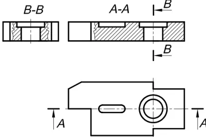
If it is beneficial to show many removed sections then the cutting planes are shown on the principal views by means of the usual symbol with arrows indicating the direction of viewing (Sections A-A, B-B, C-C) as in Fig. 3.15.

Figure 3.13 Drawing removed section by

indicating the cutting plane Figure 3.14 Drawing removed section turned by marking the cutting plane

Figure 3.15 Drawing removed sections – Cutting plane is indicated by dot-and-dash thin line.

The removed section is drawn in thick line close to the principal view in alignment and bound to the principal view with a dot-and–dash thin line (centre line). The removed section can be placed either above or below the principal view but collinear with the section plane. In this case the section plane and the removed section are not marked as in Fig. 3.16. If it is necessary the removed section may be marked as in Fig. 3.17.

(30)

30 Figure 3.16 Drawing removed

section indicated by its centre line Figure 3.17 Drawing removed section by marking the cutting

plane – The principal view is broken out.

The section plane is revolved into the drawing plane and the removed section remains in its original place. The removed section is drawn by a thick line as in Fig. 3.18.

Figure 3.18 Removed section applying broken out

Figure 3.19 Removed section revolved into the drawing plane

– The principal view is not broken out.

The section plane is revolved into the drawing plane and the removed section remains in its original place. The removed section is drawn by a thin line as in Fig.

3.19.

3.2.2 Complex sectional views

3.2.2.1 Offset sections with parallel cutting planes

Cutting planes nearly always pass through the axes of symmetry of the whole object or its detail. If several such axes of symmetry occur, the cutting plane can be offset (Fig.

3.20). Strictly speaking, the part is cut by two or more parallel planes. The two sectional views are comprised on one sectional view. A characteristic dashed line shows the offset cutting planes and arrows show the direction in which the view is taken on the end of the line. In the case of an offset sectional view the broken lines separate the sectional views to indicate the offsets of the cutting planes.

In the case of a rotation-symmetric component, if the cutting planes pass through the axis of rotation a revolved offset section can be applied by revolving the sectional views into the plane of the drawing as in Fig. 3.21 and Fig. 3.22. On the sectional view broken lines are used to indicate the cutting planes if the intersection lines of the cutting planes do not coincide with the axis of rotation. The cutting planes are shown on the drawing with the usual symbol.

(31)

31

Figure 3.20 Drawing offset section 3.2.2.2 Revolved section

A revolved section may be applied if only a part of the component is rotational-symmetric as in Fig. 3.23.

Figure 3.21 Drawing revolved offset

section Figure 3.22 Drawing revolved offset section

(32)

32

Figure 3.23 Drawing revolved section

3.2.3 Specific sectional views and sections 3.2.3.1 Developed view

If a machine part or an element thereof has a cylindrical or curved shape and its inner surface or interior construction should be represented, the developed view or developed section may be used.

Figure 3.24 Drawing developed view

By applying a developed view, representation of distorted views can be avoided. In this case the direction of viewing may be indicated by an arrow and the view has to be indicated by the symbol of developed (Fig. 3.24).

(33)

33 3.2.3.2. Developed section

Figure 3.25 Sectioning curved shape part

To represent the interior construction of a cylindrical shaped machine part, two options are available; represent several cutting planes gaining several sections (sectional views) as in Fig. 3.25 or represent a cylindrical surface as a cutting surface gaining a developed section (Fig. 3.26).

Figure 3.26 Drawing developed section

3.2.4 Conventional practice in machine drawing

The standard specifies various simplifications and conventionalities in making machine drawings.

3.2.4.1 Applying broken out section

If a visible contour line is located on the axis of symmetry (for instance an edge of a part), then the view or the section is made to be a little more than one half (as in Fig.

3.27 a, b and c) when drawing a half-sectional view.

a b c Figure 3.27 Applying broken out section on half views

(34)

34

If the cutting plane is grazing a surface of a part, this surface must not be sectioned. To avoid this, the broken-out section is used in the cutting plane as in Fig. 3.28. In this case the view is separated from the sectional view by a thin continuous freehand line.

Figure 3.28 Applying broken out section when grazing a surface

3.2.4.2 Avoiding cutting specific parts

When a section plane passes through the longitudinal axes of solid cylinders such as shafts, bolts and screws, these parts may not be cut by the section plane. Nothing would be gained by showing the solid interior of such parts, and without crosshatching large areas the drawing is clearer. Elements such as thin walls, webs, stiffening ribs, lugs, spokes of pulleys and handwheels, teeth of gears and sprockets, etc., also come under this rule. Fig. 3.29 illustrates a step bearing in section. Its stiffener is not cross-hatched even though the section plane passes through the longitudinal axis of the part and the stiffener.

Figure 3.29 Avoiding hatching webs

If webs or stiffening ribs have recesses, blind or through holes, etc., they are shown by making broken-out sections to reveal the hidden part, as in Fig. 3.30.

(35)

35

Figure 3.30 Breaking out webs

If a section plane passes through objects such as a flange (Fig. 3.31) or a flywheel (Fig.

3.32) it is conventional practice not to show the web behind the cutting plane and to represent the spoke as if turned to coincide with the section plane.

Figure 3.31 Sectioning a flange Figure 3.32 Sectioning a flywheel

3.2.4.3 Avoiding drawing transition lines

Fig. 3.33 and Fig. 3.34 indicate the conventional practice in presenting different tapers on parts. Transition lines between surfaces, gradually merging into each other, are shown conventionally or not shown at all (Fig. 3.34). This simplification can be used when the size of the drawing does not allow an accurate demonstration of the view.

Transition lines are not used for dimensioning.

Figure 3.33 Drawing transition lines Figure 3.34 Avoiding drawing transition lines

3.2.4.4 Indicating surface texture

Representing the knurled surfaces of machine parts is standardized (DIN 82) and shown, as in Fig. 3.35. Only a certain portion of such a surface is covered with the specific symbol which is limited either by outline, centre line or by free-hand drawn wave line.

(36)

36 3.2.4.5 Indicating terminal position

Terminal positions of moving components are represented by thin dot-and-dash lines as in Fig. 3.36.

Figure 3.35 Indicating surface texture Figure 3.36 Indicating terminal position

(37)

37

4. SCALES AND DIMENSIONING

4.1 Scales

The scale is the relation between the dimension of the drawing of an object and the actual dimension. Scales are defined in the standard MSZ ISO 5455.

The selected scale is appropriate if the dimension of the drawing of machine parts and assemblies is suitable for presenting their true shape and dimensions and for dimensioning. Accordingly, large objects of comparatively simple shape are drawn in smaller than full size, and small objects (such as watch parts) are scaled up.

Tabulated below are the scales used in technical drawings. All drawings should be made to scale. If several scales are used on the same drawing, the most common scale used has to be stated in the title block. However, differing scales must be shown next to the view, preferably above it.

4.1.1 Scale designation The accepted abbreviations are:

Scale 1:1 (for full size) Scale 1:5 (for scaling down)

Scale 2:1 (for scaling up), and so on.

Reduction scales: 1:2, (1:2.5), (1:4), 1:5, 1:10, (1:15), 1:20, 1:25, 1:50, (1:75) Full size: 1:1

Enlarged scales: 2:1, (2.5:1), 5:1, 10:1

The scales given in parentheses are permitted but not recommended.

4.1.2 Scale specification

If all drawings are made to the same scale, the scale should be indicated in the title block. If it is necessary to use more than one scale on a drawing, the main scale is given in the title block and all the other scales should be shown near the particular view or sectional view.

(38)

38

4.2 General instructions for dimensioning

Working drawings must indicate all necessary dimensions in a way most convenient for the workman to understand. Dimensioning methods are standardized (DIN 406; MSZ ISO 129). The size of the object or its separate parts are usually indicated in drawings by means of dimension lines, completed with numbers showing the actual measurement irrespective of the scale.

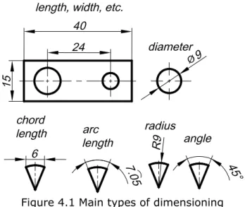
Figure 4.1 Main types of dimensioning

As a rule, dimensions in machine drawings are given in millimetres without adding the abbreviation “mm”. Dimension lines are made with thin continuous lines to contrast the thick outlines of the drawing. They are drawn parallel to the surfaces whose length they indicate and are terminated by arrowheads at the ends of the dimension line. Dimension figures must be written by standard type font to avoid confusion. They have to be written above and parallel to the dimension line leaving approximately 1 mm space from it and preferably as close to its centre as possible. Fig. 4.1 shows the main types of dimensioning.

The supplementary symbols being used in dimensioning are standardised (DIN 406 (MSZ ISO 129).

In machine drawing (working drawing, assembly drawing) the dimension pertains to the completed part. When the surface of a part has a metallic coating it pertains to the coated state, but when the surface is painted or has a plastic coating, it pertains to the state before coating (Fig. 4.2).

Figure 4.2 Indicating coated surfaces

Overall dimensions of a part have to be given. Dimensioned drawings can contain informative dimensions that are not used for manufacturing or dimensional inspection, but make it easier to read the drawing. Informative dimensions must be put in parentheses as in Fig. 4.3.

(39)

39

Figure 4.3 Chain dimensioning and informative dimensioning

However, if the drawing of a part has a break, the dimension line must be drawn without a gap, as in Fig. 3.6. Each dimension in a drawing must be given only once, duplicate dimensions have to be avoided. Dimension lines are preferably (but not obligatorily) drawn outside the drawing outlines.

The arrangement of dimensions should be carefully designed. Intersections of extension and dimension lines should be avoided. When a series of parallel dimension lines are in close proximity to each another, the space between them should be between 7 and 10 mm. Centre lines, cross-hatching lines and any other lines must be broken where arrowheads and figures are to be placed.

Arrowheads that terminate on the dimension lines must just touch the corresponding outlines, or centre lines, or extension lines (Fig. 4.4).

The size of arrowheads depends on the thickness of visible outlines. The arrowhead is about 2.5-3 mm in the case of the visible outline is 0.7 mm thick and must be the same for all dimension lines of a given drawing. Its vertex angle is 15^o (see Fig. 4.5).

Figure 4.4 Arrowhead Figure 4.5 Methods of indicating dimensions

Extension lines must extend from 2 to 3 mm beyond the ends of the arrowheads. If there is not enough space for an arrowhead because two lines of the visible outline are too close to each other, the particular outline must be broken since arrowheads must not be intersected by any lines (see Fig 4.7).

Figure 4.6 Arrangement of dimensioning

(40)

40

If there is no room for arrowheads at the ends of dimension lines arranged in a continuous chain, they may be replaced by an oblique stroke that is 2-3 mm long and has an inclination of 45° to the dimension line as in Fig 4.6.

Figure 4.7 Dimensioning half sectioned view

Figure 4.8 Dimensioning equiangular features

On half-sectioned views with an axis of symmetry it is permissible to use dimensions according to Fig. 4.7. In this case the dimension lines must extend somewhat beyond the axis of symmetry.

When dimensioning a number of equal spaced similar elements of a machine part, say, holes, proceed as in Fig. 4.8 and Fig 4.9 (usually only one hole is dimensioned and the number of holes and the spacing are indicated).

Figure 4.9 Dimensioning equidistant features

Fig. 4.10 shows how dimensions of uniform bore spacing on the same bolt circle can be given together with the diameter of the bolt circle.

Figure 4.10 Dimensioning bolt circle and holes on it

(41)

41

Squares may be dimensioned according to the size of the edge as in Fig. 4.11. The radius should always be given for dimensioning a circular part consisting of different fillets. Fig.

4.12 shows how spherical surfaces are dimensioned.

Figure 4.11 Shape identification

symbol, square Figure 4.12 Shape identification symbol, sphere

A 45^o chamfer is dimensioned using a dimension line as in Fig. 4.13 or on a leader as in Fig. 4.14.

Figure 4.13 Dimensioning chamfers Figure 4.14 Simplified chamfer dimensioning

4.2.1 Placement of dimension figures

The placements of dimensions are shown in Fig. 4.15. The basic principle is that dimension numbers should be read from the direction of the title block and from the right. Dimension numbers pertaining to the dimension lines in the hatched area have to be placed on the horizontal leader.

Fig. 4.16 shows the recommended practice for the placing of angular dimensions. An angular dimension can be placed on a horizontal leader in all cases, but in the hatched area it is compulsory.

Figure 4.15 Oblique dimensioning Figure 4.16 Angular dimensioning

(42)

42 4.2.2 Specific dimensioning

Dimension lines must not be the continuation of outlines, centre line or extension lines of any other dimensioning. Similarly, the outlines, centre lines and extension lines must not be used as dimension lines.

Although dimension lines must not be used as extension lines, they are used when dimensioning the coordinates of points on a non-circular curve (Fig. 4.17).

Figure 4.17 Dimensioning non-circular curve

If the dimension lines of a non-circular curve have a uniform spacing, the two conventional dimension types can be combined as in Fig. 4.18.

Figure 4.18 Simplified dimensioning of

non-circular curve Figure 4.19 Dimensioning non-parallel surfaces

Although extension lines should be perpendicular to the dimension lines, in certain exceptional cases extension lines may be drawn not at a right angle to dimension lines as is shown in Fig. 4.19. In this case the extension lines must be parallel to each other and they are drawn from the intersection points of the continuations of the visible outlines.

Where space limitations do not permit giving a separate line for each dimension, the dimensions may be placed in one line as shown in Fig. 4.20 and Fig. 4.21.

Figure 4.20 Simplified parallel

dimensioning Figure 4.21 Simplified parallel angular dimensioning

(43)

43

In this method, called consecutive dimensioning, there is only one arrow for each dimension, thus indicating that each dimension goes back to the original base line that is e.g. zero. In this case the dimension numbers are placed along the extension lines and the common starting point is indicated by “0” (zero) dimension.

Co-ordinate dimensioning can be performed using a table containing the coordinates (Fig.

4.22) instead of a graphical dimensional specification.

Figure 4.22 Co-ordinate dimensioning

4.2.3 Choosing reference surfaces

When dimensioning a part it is expedient to choose a reference surface in the three main directions from which the position of all the details and surfaces may be dimensioned.

Reference surfaces can be:

– a significant surface in terms of working (line marked by 1 in Fig. 4.23)

– a significant axis of symmetry in terms of working (line marked by 2 in Fig. 4.23) – boundary line/s of overall dimension/s of a stepped part (shaft), see Fig. 4.24 – boundary line of a plane or planes dimensioned from a lateral surface, Fig. 4.25 The general rule is to determine the dimensions relative to the reference surface and not to apply the closed dimension chain. However, if it is necessary derived dimensions may be put into parentheses as an informative dimension.

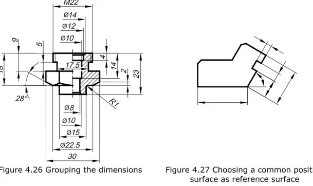
For clarity, the dimensions on the views should be grouped according to the dimensions of the inner surfaces, the outside surfaces, the finished surfaces and the unmachined surfaces as in Fig. 4.26.

(44)

44

Figure 4.23 Choosing a significant surface as a reference surface

Figure 4.24 Choosing boundary lines as reference surfaces

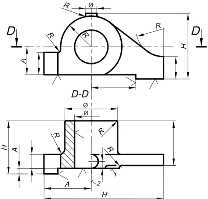
When dimensioning details on a part having common position it is expedient to choose an appropriate reference surface as in Fig. 4.27. Placement is given relative to the main directions. The dimensions of the details can be performed according to the particular reference surface.

(45)

45

Figure 4.25 Choosing several boundary lines as reference surfaces

Figure 4.26 Grouping the dimensions Figure 4.27 Choosing a common position surface as reference surface

Dimensioning of mating elements of connecting parts should be identical (i.e. the mirror image of each other, Fig. 4.28).

(46)

46

Figure 4.28 Dimensioning mating elements

4.2.4 Conventional dimensioning methods

Dimensioning of a part has to reflect the task and the significance of its surfaces in terms of working. Dimensioning is made commonly in orthogonal and rarely in the polar coordinate system.

Self evident dimensions should not be indicated in the drawing, such as:

– perpendicularity of two adjoined surfaces or edges if they are correctly drawn – parallelism of several edges or surfaces if they are correctly drawn

– equality of dimensions when halving a dimension with a centre line – vertex angle of a regular polygon

– open-end holes; a hole is always an open-end hole if the hole depth is not indicated

4.2.4.1 Conventional dimensioning practice of bore-holes a. Bore-holes with and without countersinking

Bore-hole can be threaded, without thread, open-ended holes or blind holes. Since the dimensions of the bore-hole determine its geometry, the graphical representation may be simplified and drawing a bore-hole may be omitted.

Figure 4.29 Conventional dimensioning of bore-hole

Figure 4.30 Conventional dimensioning of threaded bore-hole

(47)

47

Figure 4.31 Conventional dimensioning of threaded blind bore-hole

The bore-hole, threaded bore-hole or blind hole dimensions are given on a leader indicating the place of the centre line (Fig. 4.29, 4.30 and Fig. 4.31).

The dimensioning of the bore-hole can be completed with the simplified dimensioning of the counterbore, but the bore-hole with the counterbore has to be drawn in view and in sectional view (Fig. 4.32), as well.

Figure 4.32 Conventional dimensioning of bore-hole and threaded bore-hole with counterbore

b. Repetitive bore-holes, bore-hole groups

Dimension of identical, repetitive bore-holes may be given either on the same leader, or the bore-holes can be indicated by letters with their dimensions compiled in a table, as in Fig. 4.33.

Mark Apiece Dim.

a 6 M6x10

b 4 M8x15

c 2 Ø10

d 1 Ø12H7

Figure 4.33 Conventional dimensioning of threaded bore-hole groups

(48)

48

c. Dimensioning the length of shape rolled components and of sheet gaugenumbers The length of shape rolled materials and the sheet gauge number may be given on a leader, as in Fig. 4.34 and Fig. 4.35.

Figure 4.34 Dimensioning a shape rolled

component Figure 4.35 Dimensioning a sheet

component 4.2.5 Dimensioning tapered parts

In the case of a cone, conical taper is defined as the ratio of the diameter difference of two diameters of the cone and the distance between the two diameters as in Fig. 4.36.

Conical taper is expressed in %: D-d/L_*100. Flat taper can be defined for planes. It characterises the angle of a plane relative to another one (Fig. 4.37). Flat taper is expressed in %: A-B/L_*100.

Figure 4.36 Conical taper Figure 4.37 Flat taper

4.2.5.1 Dimensioning conical taper and flat taper

Indicating a taper by its symbol on a view is standardized (MSZ ISO 3040). The symbol is either on the centre line or on a leader parallel to the centre line, as in Fig. 4.38.

(49)

49

Figure 4.38 Dimensioning conical taper

Slant can be indicated by its symbol either on the slant line, or on a leader parallel to the reference plane of the slant, as in Fig. 4.39.

Figure 4.39 Dimensioning flat taper

The taper is given in %, but if the flat taper is bigger than 30° and the conical taper is bigger than 45°, they can be given either by the angle, or by dimensioning, as in Fig.

4.40.

Figure 4.40 Showing the taper by dimensions and angle

Figure 4.41 Giving of measuring place of tapered part

The typical dimension of the tapered or slant part is the biggest diameter or the biggest thickness. If it is difficult to measure these dimensions because of a fillet at the margin, the location of the measured point should be given, as in Fig. 4.41. Other dimensions of the tapered and slant parts are calculated from the typical dimension and

(50)

50

the given taper or slant. If a dimension is not given directly, then it is a result that has to be signed by mark as in Fig. 4.42.

Figure 4.42 Giving informative dimension signed by mark

(51)

51

5. REPRESENTATION OF THREADS AND THREADED JOINTS

Rules of machine drawing include drawing standardized parts. The application of the standardized representation facilitates drawing components and making the drawing clear and understandable.

5.1 Thread forms

Threaded fasteners (screws, bolts, nuts) should clamp parts together with a force that is big enough to hold them in contact without dislocation.

The following thread forms are in common use:

Metric threads have a sharp V profile, where the thread angle is 60°. They are widely used for bolts, screws, studs, nuts, and other fasteners.

Inch threads have a 55° triangular profile. They are used mainly for manufacturing different spare parts.

Inch taper threads have a 60^o angle. They are used in taper threaded joints of fuel, oil, water and air pipelines for various machines and machine tools.

Cylindrical pipe threads have a 55° angle with a pitch considerably smaller than that of inch thread.

Trapezoidal threads are used in different screws for driving. Its profile is trapezoidal with an angle of 30°.

Buttress threads have a profile composed of a series of non equilateral trapezium with an angle of 33°.

Standardised and practical notations and terms:

A_s Stress area of thread

D_Km Acting diameter for determining the friction torque at the fastener head or nut bearing face

FM Tension force in the fastener after completed mounting MM Tightening torque for mounting

P Thread pitch

d Fastener diameter (biggest diameter of the thread) d2 Mean flank diameter of the thread

d3 Smallest diameter of the thread



G_,



_KCoefficient of thread friction and of the fastener head or nut bearing faces

(52)

52 Property classes

The designation system for threaded fasteners consists of two numbers separated by a decimal point. The first number represents



1/100 of the ultimate tensile strength in N/mm², while the second number is 10 times the ratio of the minimum yield point to the minimum tensile strength.

The property classes of standard nuts are indicated by a number which corresponds to 1/100 of the stress under proof load in N/mm², this stress corresponds to the minimum tensile strength of a fastener in the same property class.

5.2 Conventional representation of threads

The drawing of threads is standardised (DIN 202, DIN 406 (MSZ ISO 6410). Threads are illustrated by simplified presentations according to the enveloping surface. The conventional presentation of external threads is the following: the outline of the rod, corresponding to the major diameter of the thread is drawn in continuous straight thick lines (see Fig. 5.1). Lines corresponding to the minor diameter of the thread (or lines of the roots) are drawn by continuous fine line. Internal thread in sectional view is presented by continuous visible line (the minor diameter) and continuous fine line (the major diameter), as shown in Fig. 5.2.

Figure 5.1 Conventional presentation of external threads

Figure 5.2 Conventional presentation of internal threads

Figure 5.3 Presentation of threads in

section Figure 5.4 Ignoring the presentation of the chamfer

In views perpendicular to the axis, the thread is drawn by continuous fine arc of about three-fourths of a circle. The beginning and end of the thread are presented by continuous thick lines as in Fig. 5.3. The distance between the continuous visible line and the fine line presents the thread and it is equal to the depth of thread, but it should be minimum 0.8 mm. In general only the effective length of a thread is depicted and dimensioned. If it is necessary the thread runout may be shown. In the case of a threaded blind hole, the cone angle of the hole is not of importance, it is drawn at 120°

without indicating it. Chamfers on threaded rods and holes are not shown when projected on a plane perpendicular to the axis of the rod or hole (Fig. 5.4) because they would disturb the depiction of the thread. If the chamfer of the rod is bigger than the depth of