arXiv:1708.07387v1 [math-ph] 23 Aug 2017
Volume of the space of qubit-qubit channels and state transformations under random quantum
channels ∗
Attila Lovas
†, Attila Andai Department of Analysis,
Budapest University of Technology and Economics, 1111 Budapest, Egry J´ ozsef street 1., Building H, Hungary
March 13, 2018
Abstract
The simplest building blocks for quantum computations are the qubit- qubit quantum channels. In this paper, we analyze the structure of these channels via their Choi representation. The restriction of a quantum chan- nel to the space of classical states (i.e. probability distributions) is called the underlying classical channel. The structure of quantum channels over a fixed classical channel is studied, the volume of general and unital qubit channels with respect to the Lebesgue measure is computed and explicit formulas are presented for the distribution of the volume of quantum channels over given classical channels. We study the state transformation under uniformly random quantum channels. If one applies a uniformly random quantum channel (general or unital) to a given qubit state, the distribution of the resulted quantum states is presented.
1 Introduction
In quantum information theory, a qubit is the non-commutative analogue of the classical bit. A qubit can be represented by a 2×2 complex self-adjoint positive semidefinite matrix with trace one [7, 11, 12]. The space of qubits is denoted byM2 and it can be identified with the unit ball inR3 via the Stokes parameterization. A linear map Q : M2 → M2 is called a qubit channel (or qubit quantum operation) if it is completely positive and trace preserving (CPT) [11]. A qubit channel is said to beunital (or equivalently identity preserving) if it leaves the maximally mixed state invariant.
Choi and Jamio lkowski has published a tractable representation for com- pletely positive (CP) linear maps [4, 6]. To a superoperatorQ:C2×2 →C2×2
a block matrix
Q11 Q12
Q21 Q22
Q11, Q12, Q21, Q22∈C2×2 (1)
∗quantum channel, volume; MSC2010: 81P16, 81P45, 94A17
†lovas@math.bme.hu
is associated, which is called Choi matrix, such that the action ofQis given by a b
c d
7→aQ11+bQ12+cQ21+dQ22.
Due to Choi’s theorem, the linear mapQ:C2×2→C2×2 is CP if and only if its Choi matrix is positive definite [4]. Hereafter, we will use the same symbol for the qubit channel and its Choi matrix. Clearly, a block matrix Qof the form (1) corresponds to a qubit channel if and only if Q11, Q22 ∈ M2, Q21 =Q∗12, TrQ12= 0 and Q≥0, thus the space of qubit channels can be identified with a convex subset of R12 which is denoted byQ. If we consider the set of unital qubit channels, identity preserving property requires thatQ11+Q22=I must hold in the Choi representation (1), hence the space of unital qubit channels (Q1) can be identified with a convex submanifold ofR9.
Investigation of the set Q of all qubit channels play the key role in the field of quantum information processing [7], since any physical transformation of a qubit carrying quantum information has to be described by an element of this set. Although the classical analogues ofQ andQ1 are trivial objects, the geometric properties of qubit channels are widely studied [8, 10]. However, the volume of the setsQandQ1is still unknown. Random quantum operations and especially random qubit channels are subject of a considerable scientific interest [2]. For example, an effect of external noise acting on qubits can be modeled by random qubit channels. Authors in [3] have studied the spectral properties of quantum channels and designed algorithms to generate random quantum maps.
We should mention that transformations of the maximally mixed state have important applications in superdense coding [5] which provide motivation for research on the distance of the maximally mixed state and its image under the action of a random qubit channel.
Quantum channels are non-commutative analogues of classical stochastic maps, therefore it is natural to consider their actions on classical quantum states (i.e diagonal density matrices). For a qubit channel Q, the underlying classical channel is defined as the restriction of Q to the space of classical bits. For example, the following Markov chain transition matrix represents the underlying classical channel ofQ∈ Qgiven by (1)
P =
diag(Q11) diag(Q22)
,
where diag(Qii) is a row vector that contains the diagonal of Qii.
The main aim of this paper is to compute the volume of general and unital qubit channels and investigate the distribution of the resulted quantum states if a general or unital uniformly random quantum channel was applied to a given state. To compute the volume, we follow a similar strategy to those that was introduced by Andai in [1] to calculate the volume of density matrices. This approach makes possible to gain information about the distribution of volume over classical states and to compute the effect of uniformly random quantum channels on the given state.
The paper is organized as follows. In the second Section, we fix the notations for further computations and we mention some elementary lemmas which will be used in the sequel. In Section 3, the volume of general and unital qubit channels with respect to the Lebesgue measure is computed and explicit formulas are
presented for the distribution of volume over classical channels. Section 4 deals with state transformations under uniformly random quantum channels.
2 Basic lemmas and notations
The following lemmas will be our main tools, we will use them frequently.
We also introduce some notations which will be used in the sequel.
The first two lemmas are elementary propositions in linear algebra. For an n×n matrix A we set Ai to be the left upper i×i submatrix of A, where i= 1, . . . , n.
Lemma 1. The n×n self-adjoint matrix A is positive definite if and only if the inequalitydet(Ai)>0 holds for everyi= 1, . . . , n.
Lemma 2. Assume thatAis ann×nself-adjoint, positive definite matrix with entries (aij)i,j=1,...,n and the vector x consists of the first(n−1) elements of the last column, that isx= (a1,n, . . . , an−1,n). Then we have
det(A) =anndet(An−1)− hx, T xi, whereT = det(An−1)(An−1)−1.
Proof. Elementary matrix computation, one should expand det(A) by minors, with respect to the last row.
When we integrate on a subset of the Euclidean space we always integrate with respect to the usual Lebesgue measure. The Lebesgue measure onRn will be denoted byλn.
Lemma 3. If T is ann×nself-adjoint, positive definite matrix andk, ρ∈R+, then
Z
{x∈Cn | hx,T xi<ρ}
(ρ− hx, T xi)kdλ2n(x) = πnρn+kk!
(n+k)! detT.
Proof. The set{x∈Cn | hx, T xi< ρ} is anndimensional ellipsoid, so to com- pute the integral first we transform our canonical basis to a new one, which is parallel to the axes of the ellipsoid. Since this is an orthogonal transforma- tion, its Jacobian is 1. When we transform this ellipsoid to a unit sphere, the Jacobian of this transformation is
n
Y
k=1
ρ µk
,
where (µk)k=1,...,n are the eigenvalues of T. Then we compute the integral in spherical coordinates. The integral with respect to the angles gives the surface of the 2n dimensional sphere that is 2πn
(n−1)!r2n−1. The integral of the radial part is
Z 1 0
2πn
(n−1)!r2n−1 ρn
detT(ρ−ρr2)kdr= 2πnρn+k (n−1)! detT
Z 1 0
r2n−1(1−r2)k,dr which gives back the stated formula.
Lemma 4. Assume thatX is a spherically symmetric and continuous random variable which takes values in the unit ball {x∈ R3 : kxk ≤ 1}. If f denotes the probability density function of thezcomponent ofX, then for the density of kXk we have
ρ(r) =−2rf′(r) r∈]0,1[. (2) Proof. Let us denote by fX the probability density function of X in the unit ball. The distribution of X is rotation invariant thus there exists a function g: [0,1]→R+ such that, for everyxin the unit ballfX(x) =g(kxk). For the radial density we have
ρ(r) = d
drP(kXk< r) = d dr4π
r
Z
0
g(s)s2ds= 4πg(r)r2 r∈]0,1[.
Now we compute the density function of thez component from the radial dis- tribution. For everyz0∈]0,1[
f(z0) = d dz0
P(z < z0) =− d dz0
P(z≥z0)
=− d dz0
2π
Z
0 1
Z
y
arccos(z0/r)
Z
0
g(r)r2sinφdφdrdθ= 2π
1
Z
z0
g(r)rdr
holds and from this by derivation we get
f′(r) =−2πg(r)r=−ρ(r) 2r , which completes the proof.
3 The volume of qubit channels
To determine the volume of different qubit quantum channels we use the same method which consists of three parts. First, we use a unitary transforma- tion to represent channels in a suitable form for further computations. Then we split the parameter space into lower dimensional parts such that the adequate applications of the previously mentioned lemmas lead us to the result.
3.1 General qubit channels
The following parametrization ofQ ⊂R12 is considered
Q=
a1 b c d
¯b a2 e −c
¯
c ¯e f1 g d¯ −¯c g¯ f2
, (3)
wherea1, f1∈[0,1],a2= 1−a1,f2= 1−f1 andb, c, d, e, g∈C. Let us define a=a1and f =f1.
The underlying classical channel corresponding to these parameter values are given byQcl=
a 1−a f 1−f
. Let us choose the unitary matrix
U =
1 0 0 0 0 0 1 0 0 1 0 0 0 0 0 1
(4)
and define the matrixA as
A=U∗QU =
a c b d
¯
c f e¯ g
¯b e a2 −c d¯ ¯g −c¯ f2
, (5)
which is positive definite if and only ifQis positive definite.
Theorem 1. The volume of the space Q with respect to the Lebesgue measure is
V(Q) = 2π5 4725
and the distribution of volume over classical channels can be written as
V(a1, f1) =24π5 45
a31f13(a21f12−5a1a2f1f2+ 10a22f22) if a1+f1≤1, a32f23(a22f22−5a1a2f1f2+ 10a21f12) if a1+f1>1.
(6) Proof. Since there is an unitary transformation (4) between the set of matrices of the form of (5) and the quantum channels their volumes are the same. We compute the volume of the set of matrices given by parameterization (5).
The volume element corresponding to the parametrization (3) is 27dλ12. The matrixA in Equation (5) is positive definite if and only if det(Ai)>0 for i= 1,2,3,4.
First we assume that the parameters a, f and the submatrix A3 are given and consider the requirement detA4 ≥ 0. Simple calculation shows that we have
detA4=R3− d′
g′
, T3 d′
g′
,
whered′=d+ bc a2
,g′=g+c¯e a2
,R3= (detA3) f2−|c|2 a2
! and
T3=
a2f1− |e|2 be−a2c
¯b¯e−a2¯c a1a2− |b|2
.
In this case the inequality detA4≥0 can be written in the form of d′
g′
, T3
d′ g′
≤R3. (7)
The matrix T3 is positive, because detT3 = a2detA3 ≥ 0 and (T3)11 is the determinant of the middle 2×2 submatix ofA. It means, that the Inequality (7) has solution if, and only iff2a2≥ |c|2.
The transformation (d, g)7→ (d′, g′) is a shift, therefore it does not change the volume element. We have by Lemma 3
V(a, f, b, c, e) = 27
Z
d′ g′
,T3
d′ g′
≤R3
1 d(d′, g′) = 26R32π2 detT3
,
where detT3=a2detA3, therefore
V(a, f, b, c, e) =
26π2
a32
a2f2− |c|22
detA3 if f2a2≥ |c|2, 0 if f2a2<|c|2.
In the second step we assume that the parameters a, f and the submatrix A2 are given and consider the requirement detA3≥0. We have
detA3=R2− b
¯ e
, T2
b
¯ e
, whereR2= (1−a) detA2 and
T2=
f −c
−c¯ a
. The inequality detA3≥0 can be written in the form of
b
¯ e
, T2
b
¯ e
≤R2.
We now integrate with respect tob ande. To compute the integral V(a, f, c) =
Z
b
¯ e
,T2
b
¯ e
≤R2
V(a, f, b, c, e) d(b, e)
=
Z
b
¯ e
,T2
b
¯ e
≤R2
f2a2≥c2
26π2 a32
a2f2− |c|22
detA3d(b, e)
we substitute detA3=R2− b
¯ e
, T2
b
¯ e
and by Lemma 3 we have
V(a, f, c) = 26π2 a32
a2f2− |c|22 Z
b
¯ e
,T2
b
¯ e
≤R2
R2−
b
¯ e
, T2
b
¯ e
d(b, e)
= 26π2 a32
a2f2− |c|22
× π2R32 6 detT2
,
where detT2= detA2, therefore
V(a, f, c) =
25π4
3
a2f2− |c|22
×(detA2)2 if f2a2≥ |c|2, 0 if f2a2<|c|2.
In the final step we assume that the parametersa, f are given and consider the requirement detA2≥0. It means that|c|2≤af, therefore if
|c|2≤min{af,(1−a)(1−f)} then
V(a, f, c) = 25π4 3
a2f2− |c|22
×
af− |c|22
.
Ifa+f ≤1, thenaf ≤(1−a)(1−f). In this case using polar coordinates for cwe have
V(a, f) = 2π
√af
Z
0
25π4
3 a2f2−r22
af−r22
×rdr
=24π5
45 a31f13(a21f12−5a1a2f1f2+ 10a22f22). (8) Ifa+f ≥1, thenaf ≥(1−a)(1−f). In this case using polar coordinates for cwe have
V(a, f) = 2π
√(1−a)(1−f)
Z
0
25π4
3 a2f2−r22
af−r22
×rdr
=24π5
45 a32f23(a22f22−5a1a2f1f2+ 10a21f12). (9) Equations (8) and (9) give back Equation (6). The volume of the space of quantum channels is
V = Z 1
0
Z 1 0
V(a, f) dadf = 2π5
4725. (10)
3.2 Unital qubit channels
The following parametrization ofQ1⊂R9is considered
Q=
a1 b c d
¯b a2 e −c
¯
c ¯e a2 −b d¯ −¯c −¯b a1
, (11)
where a1 ∈ [0,1], a2 = 1−a1 and b, c, d, e ∈ C. Let us define a =a1. The underlying classical channel corresponding to these parameter values are given
byQ1cl=
a 1−a 1−a a
. Let us choose the unitary matrix
U=
0 0 1 0
1 0 0 0
0 1 0 0
0 0 0 1
(12)
and define the matrixAas
A=U∗QU =
a2 e ¯b −c
¯
e a2 ¯c −b
b c a1 d
−¯c −¯b d¯ a1
, (13)
which is positive definite if and only if Qis positive definite.
Theorem 2. The volume of the space Q1 with respect to the Lebesgue measure is
V(Q) =8π4 945
and the distribution of volume over classical channels can be written as
V(a) =24π4
3 a4(1−a)4. (14)
Proof. Since there is an unitary transformation (12) between the set of matrices of the form of (13) and the quantum channels, their volumes are the same. We compute the volume of the set of matrices given by parameterization (13).
The volume element corresponding to the parametrization (11) is 27dλ12. The matrixAin Equation (13) if positive definite if and only if det(Ai)>0 for i= 1,2,3,4.
First we assume that the parameter aand the submatrix A3 are given and consider the requirement detA4≥0. Simple calculation shows that we have
detA4= (detA3)2
detA2 − |d′|2detA2, where
d′=d+2bc(1−a)−ec¯ 2−b2e detA2
.
In this case the inequality detA4≥0 can be written in the form of
|d′| ≤ detA3
detA2
.
The transformationd7→d′ is a shift, therefore it does not change the volume element. So we have
V(a, b, c, e) = Z
|d′|≤detdetA3A2
27d(d′) = 27π
detA3
detA2
2
.
In the next step we assume that the parameteraand the submatrixA2are given and consider the requirement detA3≥0. We have
detA3=R2− ¯b
¯ c
, T2
¯b
¯ c
, where
R2=A33detA2 and T2=
a2 −e
−e¯ a2
. The inequality detA3≥0 can be written in the form of
¯b
¯ c
, T2
¯b
¯ c
≤R2.
We now integrate with respect tobandc. To compute the integral V(a, e) =
Z
¯b
¯ c
,T2
¯b
¯ c
≤R2
V(a, b, c, e) d(b, c)
=
Z
¯b
¯ c
,T2
¯b
¯ c
≤R2
27π
detA3
detA2
2
d(b, c)
we substitute detA3=R2− ¯b
¯ c
, T2
¯b
¯ c
and by Lemma 3 we have
V(a, e) = 27π (detA2)2
Z
¯b
¯ c
,T2
¯b
¯ c
≤R2
R2−
¯b
¯ c
, T2
¯b
¯ c
2
d(b, c)
=25π3a4
3 ×detA2.
Finally we assume that the parameterais given and consider the requirement detA2 ≥0. The condition detA2 ≥0 means that|e| ≤1−a, therefore using polar coordinates forewe have
V(a) = 2π Z 1−a
0
25π3a4
3 ×((1−a)2−r2)×rdr=24π4
3 a4(1−a)4, which gives back Equation (14). The volume of the space of unital quantum channels is
V = Z 1
0
V(a) da=8π4 945.
One might think about the generalization of the presented results, although in a more general setting several complications occur. For example, in the case of unital qubit channels one should integrate on the Birkhoff polytope, which would cause difficulties since even the volume of the polytope is still unknown [9].
4 State transformations under random channels
In this point, we study how qubits transform under uniformly distributed random quantum channels with respect to the Lebesgue measure. For sim- plification in this Section uniformly means that uniformly with respect to the Lebesgue measure.
For further calculations, we need the Pauli basis representation of qubit channels. The Pauli matrices are the following.
σ1= 0 1
1 0
σ2=
0 i
−i 0
σ3= 1 0
0 −1
We use the Stokes representation of qubits which gives a bijective correspon- dence between qubits and the unit ball inR3 via the map
x∈R3| kxk2≤1 → M2 x7→ 1
2(I+x·σ), wherex·σ=
3
X
j=1
xiσi andI= 1 0
0 1
. The vectorx, which describes the state called Bloch vector and the unit ball in this setting is called Bloch sphere.
Any trace-preserving linear map Q : C2×2 → C2×2 can be written in this basis as
Q 1
2(I+x·σ)
= 1
2(I+ (v+T x)·σ),
where v∈R3 and T is a 3×3 real matrix. Necessary and sufficient condition for complete positivity of such maps are presented in [12]. If the Choi matrix of qubit channel is given by Equation (3), then the Pauli basis representation has the following form.
v=
Re(b+g)
−Im(b+g) a+f−1
T =
Re(d+e) Im(d+e) Re(b−g) Im(e−d) Re(d−e) Im(g−b)
2Re(c) 2Im(c) a−f
(15) The next lemma expresses the simple fact that uniformly distributed qubit- qubit channels have no preferred direction according to the Stokes parameteri- zation of the state space.
Lemma 5. An orthogonal orientation preserving transformation O in R3 in- duces maps αO, βO : Q → Q via Stokes parametrization αO(Q) = O◦Q and βO(Q) =Q◦O. The Jacobian of these transformations are 1. The Jacobian of the restricted transformationsα′O=αO
Q1 andβO′ =βO
Q1 are 1.
Proof. We used a computer algebra program to verify this lemma. We consid- ered three different kind of rotations according to the plane of rotations (xy,xz and yz plane). It is enough to prove that the Jacobian of the generatedα, β transformation is 1, since every orthogonal orientation preserving transforma- tion can be written as a suitable product of these elementary rotations. We present the calculations forβ0, where
O=
1 0 0
0 cosα −sinα 0 sinα cosα
α∈R.
If we consider a quantum channel given by parameters as in Equation (3), then the effect ofβO can be computed
βO(a, f, b1, b2, c1, c2,d1, d2, e1, e2, g1, g2)
= (a′, f′, b′1, b′2, c′1, c′2, d′1, d′2, e′1, e′2, g′1, g2′),
where all the parameters are real numbers and subscript 1 refers to the real part and 2 to the imaginary part. We list some of the new parameters.
a′= a+f
2 +(a−f) cosα
2 +c2sinα f′= a+f
2 −(a−f) cosα
2 −c2sinα b′1= b1(1 + cosα) +g1(1−cosα)
2 +(e2+d2) sinα 2 b′2= b2(1 + cosα) +g2(1−cosα)
2 + +(e2−d2) sinα 2 c′1=c1
c′2=c2cosα−(a−f) sinα 2
Next we computed the 12×12 coefficient matrix, which is the derivative of the function β0, and the computed determinant of the coefficient matrix turned to be 1. The similar computation was done for the other rotations. The Jacobian of transformationsα0,α′O andβO′ was checked similarly.
The idea of calculations about state transformations under random quantum channel is presented by the following simpler case.
Theorem 3. Applying uniformly random channels to the most mixed state, the radii distribution of the resulted quantum states is the following.
κ(r) = 40r2(1−r)6(r3+ 6r2+ 12r+ 2) r∈[0,1] (16) Proof. Applying a quantum channel of the form of given by Equation (3) to the most mixed state giveszcomponentz′=a+f−1. Ifz≥0 then take the (not normalized) distribution from Equation (6)
V˜(a, f) = (1−a)3(1−f)3 (1−a)2(1−f)2−5a(1−a)f(1−f) + 10a2f2 . The density function of thez component comes from the integral
η(z)∼
1
Z
z
V˜(a, z+ 1−a) da.
Thez <0 case can be handled in a similar way. After normalization we have the following formula for the density function.
η(z) = 20 11
z4+ 7|z|3+ 17z2+ 7|z|+ 1
(1− |z|)7 z∈[−1,1] (17) The distribution of quantum channels is invariant for orthogonal transforma- tions (Lemma 5, the Jacobian ofαOis 1). This means, that for every orthogonal
basis the distribution of thez component of the image of the maximally mixed state is given by Equation (17). Using Lemma 4 we have
κ(r) =−2rη′(r), which gives the desired formula forκimmediately.
It is worth to note that contrary to the classical case in quantum setting the entropy of the most mixed state will decrease after a random quantum channel is applied, since the Bloch radius of the resulted quantum state is 50
143 in average.
Now we study the effect of unital uniformly distributed quantum channels.
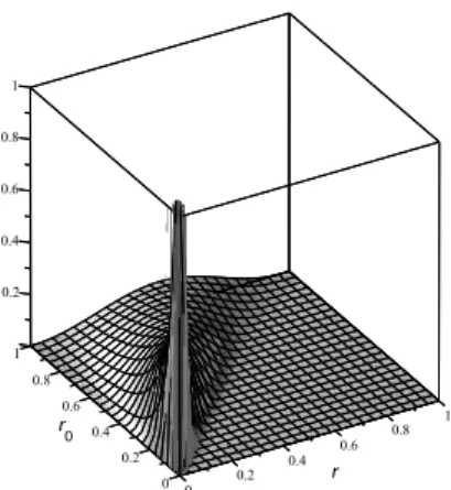
Theorem 4. Assume that uniformly distributed unital quantum channel is ap- plied to a given state with Bloch radiusr0. The radii distribution of the resulted quantum states is the following.
κ1(r, r0) =315
16 ×r2(r20−r2)3
r09 χ[0,r0](r) r∈[0,1]. (18) Proof. Since the distribution of unital uniform quantum channels is invariant for orthogonal transformations (Lemma 5, the Jacobian ofβO′ is 1), we can assume that the initial state was given by the vector (0,0, r0) (r0∈]0,1]). Applying a unital quantum channel of the form of (11) to the initial state, we get a state withz component z′ =r0(2a−1). The density function of the parametera of uniformly distributed unital quantum channels is a normalized form of (14)
V˜(a) = 630a4(1−a)4 a∈[0,1]. Ifz∈[−1,1] arbitrary, then
P(z′< z) =P
a <z+r0
2r0
=
0 if z≤ −r0,
(z+r0)/(2r0)
Z
0
V˜(a) da if −r0< z < r0, 1 if z≥r0. We have for the density function of the zcomponent
fr0(z) = dP(z′ < z)
dz =315
256×(r20−z2)4
r90 χ[−r0,r0](z),
whereχdenotes the characteristic function. If the distribution of thezcompo- nent is known then by Lemma 4 we can compute the radial distribution which gives us Equation (18).
The transition probability between different Bloch radii under uniformly distributed unital quantum channels κ1(r, r0) is shown in Figure 1. As it is expected, a unital quantum channel decreases the initial Bloch radius r0, the new Bloch radius is 63
128r0 in average. Since r′ ∼ r
2, repeated application of uniformly distributed unital quantum channels maps every initial state to the most mixed state and the convergence is exponential.
Figure 1: The function κ1(r, r0). That is the radii distribution (r) of the resulted quantum states if uniformly distributed unital quantum channels were applied to a given state with Bloch radiusr0.
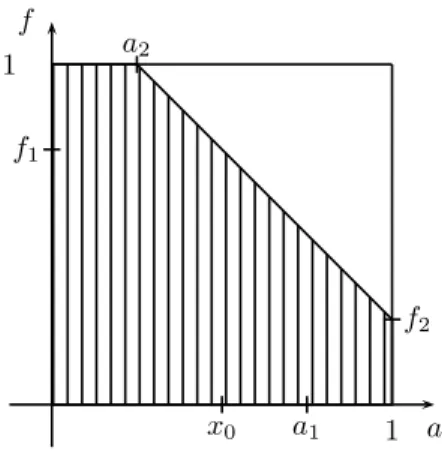
Theorem 5. Assume that uniformly distributed quantum channel is applied to a given state with Bloch radiusr0. The radii distribution of the resulted quantum states is the following.
κ(r, r0) =
If 0< r≤r0: 40r2
r0(1 +r0)6(21r4−6r2r20−36r2r0+r04+ 6r30+ 12r20+ 2r0), if r0< r≤1:
40r(r−1)6
(1−r20)6 (21r04−6r2r20−36rr20+r4+ 6r3+ 12r2+ 2r).
(19) Proof. Since the distribution of unital quantum channels is invariant for orthog- onal transformations (Lemma 5, the Jacobian ofβO′ is 1) we can assume that the initial state was given by the vector (0,0, r0) (r0∈]0,1]). Applying a quantum channel of the form of (3) to the initial state, we get a state withzcomponent z′=a+f−1 +r0(a−f). The density function of parametersa, f of uniformly distributed quantum channels is a normalized form of (6)
V˜(a, f) =
Vu(a, f) if 1≤a1+f1, Vl(a, f) if 1> a1+f1, where
Vu(a, f) = 840(1−a)3(1−f)3((1−a)2(1−f)2−5a(1−a)f(1−f) + 10a2f2) Vl(a, f) = 840a3f3(a2f2−5a(1−a)f(1−f) + 10(1−a)2(1−f)2).
First, we compute the probabilityP(z′< ξ), whereξ∈[−1,1] is an arbitrary parameter. To determine the probabilityP(z′< ξ) the solution of the inequality
z′ =a+f −1 +r0(a−f)< ξ
is needed for every parameterr0∈]0,1] andξ∈[−1,1], taking into account the constraints 0≤a, f≤1.
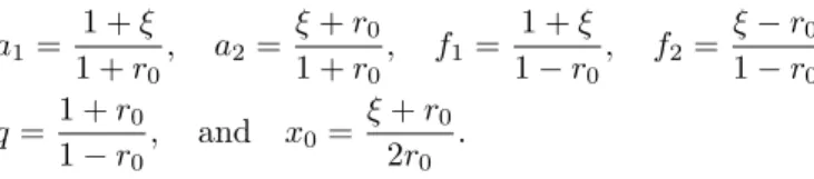
To simplify this computation we define temporarily a1= 1 +ξ
1 +r0
, a2= ξ+r0
1 +r0
, f1= 1 +ξ 1−r0
, f2=ξ−r0
1−r0
q=1 +r0
1−r0
, and x0= ξ+r0
2r0
.
In the ξ < −r0 case to compute the probability P(z′ < ξ) we have to integrate the density function ˜V(a, f) over the marked area shown in Figure 2.
a f
1 1
a1
x0
a2
f1
f2
Figure 2: Solution of the inequalityz′< ξ in the ξ <−r0 case.
P(z′< ξ) = Z a1
0
f1−aq
Z
0
Vl(a, f) dfda=
(10ξ4−88ξ2r20+ 495r40−80ξ3+ 704ξr20+ 228ξ2−198r20−144ξ+ 33)(1 +ξ)8 66(1−r20)6
In the −r0 ≤ ξ ≤ r0 case to compute the probability P(z′ < ξ) we have to integrate the density function ˜V(a, f) over the four marked areas shown in Figure 3. That is
P(z′< ξ) =
x0
Z
0 1−a
Z
0
Vl(a, f) dfda+
a1
Z
x0
f1−aq
Z
0
Vl(a, f) dfda
+
a2
Z
0 1
Z
1−a
Vu(a, f) dfda+
x0
Z
a2
f1−aq
Z
1−a
Vu(a, fdfda
a f
1 1
a1
x0
a2
f1
f2
Figure 3: Solution of the inequality z′ < ξin the −r0≤ξ≤r0case.
which gives us
P(z′< ξ) = −1
66r0(1 +r0)6(660ξ7−396ξ5r02+ 220ξ3r40−100ξr60−33r70
−2376ξ5r0+ 1320ξ3r03−600ξr05−198r60+ 2640ξ3r20−1440ξr04−495r50 + 440ξ3r0−1640ξr03−660r40−720ξr20−495r03−120ξr0−198r02−33r0).
Finally in the ξ > r0 case to compute the probabilityP(z′ < ξ) we have to integrate the density function ˜V(a, f) over the marked area shown in Figure 4.
a f
1 1
a1
x0
a2
f1
f2
Figure 4: Solution of the inequalityz′< ξ in theξ > r0 case.
P(z′< ξ) = 1−
1
Z
a2
1
Z
f1−aq
Vu(a, f) dfda= 1−
(10ξ4−88ξ2r02+ 495r40+ 80ξ3−704ξr20+ 228ξ2−198r20+ 144ξ+ 33)(1−ξ)8 66(1−r20)6
Now we can compute the density function of thez component as fz(ξ) = dP(z′< ξ)
dξ .
Since the density function is even (fz(ξ) =fz(−ξ)), we consider only theξ≥0 case. Ifξ > r0, we have
fz(ξ) = 20(1−ξ)7
33(1−r0)6(3ξ4−22ξ2r20+ 99r04+ 21ξ3−154ξr20+ 51ξ2−22r20+ 21ξ+ 3) and if 0≤x≤r0, then
fz(ξ) = −10
33r0(1 +r0)6(231ξ6−99ξ4r20+ 33ξ2r40−5r06−594ξ4r0+ 198ξ2r30
−30r05+ 396ξ2r20−72r40+ 66ξ2r0−82r30−36r20−6r0).
Now we have the distribution of thez component and by Lemma 4 we can get the radial distributionκ(19).
The transition probability between different Bloch radii under uniformly distributed channelκ(r, r0) is shown in Figure 5.
Figure 5: The functionκ(r, r0). That is the radii distribution (r) of the resulted quantum states if uniformly distributed quantum channels were applied to a given state with Bloch radiusr0.
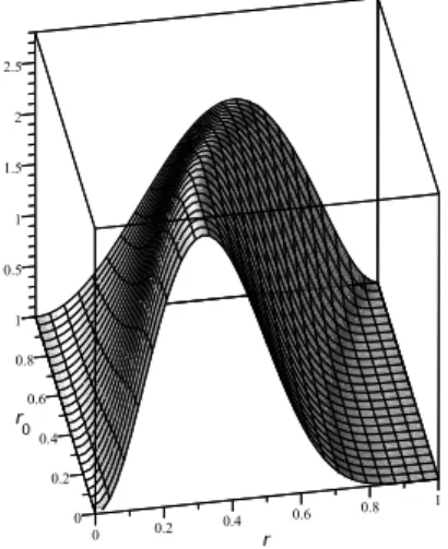
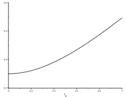
Note that the function κ(r,0) gives back the formula (16) in Theorem 3. In Figure 6 the average Bloch radius is shown after uniformly distributed random quantum channel applied to a state with Bloch radius r0. From this figure it is clear that if the initial Bloch radius is small then a quantum channel likely increases the Bloch radius and ifr0 is big then decreases. Repeated application of such kind of random quantum channels will send initial states to the Bloch radiusr≈0.388.
Figure 6: The average Bloch radius after uniformly distributed random quantum channel applied to a state with Bloch radiusr0.
5 Concluding remarks
In this work we considered the Choi representation of quantum channels and the Lebesgue measure on matrix elements. We computed the volume of quan- tum channels and studied the effect of uniformly randomly distributed (with respect the Lebesgue measure) general and unital qbit-qbit quantum channels using the Choi’s representation. It was shown that the chosen measure on the space of qbit-qbit channels is unitary invariant with respect to the initial and final qbit spaces separately. We presented the Bloch radii distributions of states after a uniformly random general or unital quantum channel was applied to a given state. This gives opportunity to study the distribution of different infor- mation theoretic quantities (for example different channel capacities, entropy gain, entropy of channels etc.) and the effect of repeated applications of uni- formly random channels.
References
[1] A. Andai. Volume of the quantum mechanical state space. Journal of Physiscs A: Mathematical and Theoretical, 39:13641–13657, 2006.
[2] J. Bouda, M. Koniorczyk, and A. Varga. Random unitary qubit channels:
entropy relations, private quantum channels and non-malleability. The European Physical Journal D, 53(3):365–372, 2009.
[3] W. Bruzda, V. Cappellini, H.-J. Sommers, and K. Zyczkowski. Random quantum operations. Physics Letters A, 373(3):320–324, 2009.
[4] M.-D. Choi. Completely positive linear maps on complex matrices. Linear Algebra and Appl., 10:285–290, 1975.
[5] A. Harrow, P. Hayden, and D. Leung. Superdense coding of quantum states. Phys. Rev. Lett., 92(18), 2004.
[6] A. Jamio l kowski. Linear transformations which preserve trace and positive semidefiniteness of operators.Rep. Mathematical Phys., 3(4):275–278, 1972.
[7] M. A. Neilsen and I. L. Chuang. Quantum Computation and Quantum Information. Cambridge University Press, Cambridge, 2000.
[8] S. Omkar, R. Srikanth, and Subhashish Banerjee. Dissipative and non- dissipative single-qubit channels: dynamics and geometry.Quantum Infor- mation Processing, 12(12):3725–3744, 2013.
[9] Igor Pak. Four questions on birkhoff polytope. Annals of Combinatorics, 4(1):83–90, 2000.
[10] A. Pasieka, D. W. Kribs, R. Laflamme, and R. Pereira. On the geometric interpretation of single qubit quantum operations on the bloch sphere.Acta Appl. Math., 108(697), 2009.
[11] D. Petz. Quantum Information Theory and Quantum Statistics. Springer, Berlin-Heidelberg, 2008.
[12] M. B. Ruskai, S. Szarek, and E. Werner. An analysis of completely positive trace- preserving maps onM2. Linear Algebra Appl., 347:159–187, 2002.