Learning to Generate Ambiguous Sequences

(1)

Learning to Generate Ambiguous Sequences

David Iclanzan and László Szilágyi Sapientia University, Târgu-Mure¸s, Romania

david.iclanzan@gmail.com

Abstract. In this paper, we experiment with methods for obtaining binary sequences with a random probability mass function and with low autocorrelation and use it to generate ambiguous outcomes.

Outputs from a neural network are mixed and shuﬄed, resulting in binary sequences whose probability mass function is non-convergent, con- stantly moving and changing.

Empirical comparison with algorithms that generate ambiguity shows that the sequences generated by the proposed method have a significantly lower serial dependence. Therefore, the method is useful in scenarios where observes can see and record the outcome of each draw sequentially, by hindering the ability to make useful statistical inferences.

Keywords: neural networks·generative adversarial networks ·objective ambiguity·Knightian uncertainty

1 Introduction

Many real world processes involve a high degree of uncertainty and modelling them is an important and challenging aspect of the analysis of complex systems.

Typically it is assumed that uncertainty should be modelled in the form of risk, where the uncertainty can be described with a probability distribution. However, uncertainty is a complex concept that goes beyond risk; there are also unpredictable events where probabilities cannot be assigned to the possible outcomes.

[9] explicitly distinguishes risk from so called Knightian uncertainty, on the basis of whether (objectively or subjectively derived) probabilistic information about the possible outcomes is present or not.

For example, if urnAcontainsnred and blue balls in equal proportion while urnBcontainsntotal red and blue balls but the number of each is unknown: (i) the probability of drawing a red ball from urnAis 1/2; (ii) no such probability can be assigned in the case of urnB.

Looking at the sources of unpredictability, we can distinguish between ignorance, where probabilistic information about the external events that aﬀect the outcomes are withheld or hidden; and true ambiguity, where there is a lack of any quantifiable knowledge about the possible occurrences [6].

Typically, experiments that need to convey uncertainty[3] have chosen to achieve this by withholding information; here an objective probability exists, but the subjects are placed in a state of unawareness, they lack the suﬃcient information to infer a probabilistic.

(2)

Withholding information can become diﬃcult in experiments involving rep- etition as experience can reduce subjects ignorance. Therefore, there are also eﬀorts to generate so called objective ambiguity in the laboratory [13] where true probabilities are incognizable to the subjects, even with arbitrarily large numbers of repetitions. In the devised process, even the experimenter, with full knowledge of the operations involved does not have a way to assess the probability distribution of the outcomes.

Extensive evidence corroborate that subjects behave diﬀerently under Knigh- tian uncertainty and risk. Specifically, most subjects are ambiguity averse, as exemplified in the Ellsberg Paradox [3]. Other results show that Knightian uncertainty can be used in games strategically to gain an advantage [11], given that the other players are ambiguity averse.

Ambiguity averse behaviour can be explained by the maxmin expected utility model [4], where one maximizes the minimum utility across diﬀerent probability distributions. Here, players focus on worst-case scenarios to determine their op- timal decisions. However, even if ambiguity aversion may usually prevail among players, there are also other behaviours and choices that occur in situations that feature ambiguity [12,8]. Focusing exclusively on worst-case scenarios may place an excessive and unrealistic limitation on the domain of admissible individual preferences in the presence of ambiguity[7]. This is especially true in the case of objective ambiguity devices, whose properties can be freely studied. In the case of these devices, a subject could learn form experience, that the setup is not adversarial, and assuming the worst case scenario is not the most appropriate.

If subjects are not averted by the fact that the precise probability of outcomes stay unknown, there still remains quantifiable and exploitable knowledge about the possible occurrences. By definition, if the outcomes do not follow the uniform probability distribution, the entropy is not maximal, there might be useful information that could be used to gain an advantage. For example, in the objective ambiguity generation process described in [13] there is a strong serial dependence between realizations. In experiments where one can observe each realization as it is made, a savvy agent could infer which outcomes have a higher probability than others; that is an exploitable edge even if the true exact probabilities remain unknowable.

In order to induce ambiguity aversion in a larger spectrum of subjects, data coming from an objective ambiguity generation processes should (i) have a divergent cumulative distribution function; (ii) be non-predictable not just in the sense that the exact probability of outcomes are impossible to known taking into account past data, but also in a stronger sense, where it is hard to identify outcomes more likely to occur in the short term than the others.

To achieve the above desiderates, in this paper we fuse a neural network’s outputs for ambiguity generation. We train a neural network as generative model, to transform noise into binary sequences with low autocorrelation. The outputs of the network are combined to obtain binary sequences with a divergent cumulative distribution function and low serial dependence.

(3)

2 Background

2.1 Compound lotteries

The simplest way to induce ambiguity, is to generate a distributions of balls in an Ellsberg-type urn using a uniform distribution over possible ratios of the balls [1]. For example, if rand() is a function to generate a number according to a uniform distribution, then an ambguous bit can be generated with the b=rand()<rand() expression.

This method is suitable just for one-shot experiments. It is not suitable for repeated outcomes as the cumulative distribution function of the generated series is not divergent.

2.2 Objective ambiguity

[13] introduces a data generating process in which the cumulative distribution function is divergent, and for which it is not possible to infer any quantile or moment of the underlying distribution.

The method is centred around three building blocks:

1. A process with a unit root, that leads to divergence as the number of draws becomes large.

2. A Cauchy distribution for individual draws, , which is a distribution without any integer moments.

3. Controlling the scale of the Cauchy distribution, to prevent the process from diverging too quickly.

The Cauchy distribution is defined as F(x) = 1

πarctan(x−x0

γ ) +1

2 (1)

wherex0 is called the location of the distribution, andγ is the scale.

The parametrized distribution is denoted byC[x0,γ].

The trick is that the realized draws are used to shift the location and scale of the distribution, making the process non-stationary (giving the process a unit root). Whenγis small the location is usually shifted slowly, but large draws also materialize, that induce a larger jumps.

Let capital letters denote random variables, lower case letters realizations andφ,ψ∈(0,1) two parameters, both small. Formally, the procedure described in [13] works as follows:

1. Draw Z0∼C[0,1]

2. Draw Z1∼C[z0,1]

3. Fort≥2 drawZt∼C[z_t−1,φ|z_t−1|+ψ]

(4)

Binary outcomes are generated, by checking if the greatest integer no larger thanztis even or odd:bt=⌊zt⌋mod2.

The procedure alternates between stable and volatile phases. Whenγis small, the generated values tend to stay close together (stable period). When an extreme realization arrives that is far from x0, it is embedded into the scale pa- rameter two draws later. This increases the chance that subsequent draws are also far from the location, causing the process to shift to an unstable period, until a draw with a small absolute value arrives again, causing the scale to be reduced again. The period lengths are unpredictable.

The cumulative sums of some sample runs, containing 10e4 binary outcomes generated according to the above described process, are shown in fig. 1. Zero values have been replaced with -1 to make the ratio of the two possible outcomes more easily assessable visually. The 0X axis is depicted with a red line. We can observe that the cumulative sums do not converge and the stable and extreme periods alternate randomly.

We can also observe that the data is serially dependent, there are long periods when the process only generates one kind of output. Fig. 2 shows the sample autocorrelation function (ACF) of the runs, with lagk= 20. Autocorrelation is very high, close to 1 for all lags, in almost every run.

-2.5 -2 -1.5 -1 -0.5 0104

-2 -1 0 1 2 3104

-1 0 1 2 3104

-2 -1 0 1 2 3 4104

-2 -1.5 -1 -0.5 0 0.5 1 104

-5000 0 5000 10000 15000

-2 -1.5 -1 -0.5 0 0.5 1 104

-4000 -2000 0 2000 4000

-2 -1 0 1 2 3104

-2000 0 2000 4000 6000 8000 10000

-6 -4 -2 0 2104

-3 -2 -1 0 1 2104

-1 0 1 2 3104

-2 0 2 4 6 8 10104

-5 -4 -3 -2 -1 0 1104

-2 -1.5 -1 -0.5 0 0.5 1104

-4 -3 -2 -1 0 1 2104

-1 0 1 2 3 4 5104

-2.5 -2 -1.5 -1 -0.5 0104

-5000 0 5000 10000

0 2 4 6 8 10

104 -2

-1 0 1 2104

0 2 4 6 8 10

104 0

0.5 1 1.5 2 2.5 3104

0 2 4 6 8 10

104 -1

-0.5 0 0.5 1 1.5 2104

0 2 4 6 8 10

104 -2

0 2 4 6 8104

0 2 4 6 8 10

104 -0.5

0 0.5 1 1.5 2 2.5104

Fig. 1. Cumulative sums of sample runs. Stable and extreme periods alternate randomly.

To hinder the ability to exploit the serial dependence, resulting from whether the process is in a calm or unstable period, the authors in [13] propose to reme- dies.

The first one requires to randomly permute the original sequence, and present the data in the randomly garbled order. While this approach destroys the autocorrelation it also introduces a look ahead bias as depicted in fig. 3. With

(5)

0 0.2 0.4 0.6 0.8 1

Lag

0 0.2 0.4 0.6 0.8 1

0 5 10 15 20

Lag 0 0.2 0.4 0.6 0.8 1

0 5 10 15 20

Lag 0 0.2 0.4 0.6 0.8 1

0 5 10 15 20

Lag 0 0.2 0.4 0.6 0.8 1

0 5 10 15 20

Lag 0 0.2 0.4 0.6 0.8 1

0 5 10 15 20

Lag

Fig. 2.Sample ACF of the example runs from fig. 1. Values are close to 1 for all lags, in almost every run.

the random shuﬄe the amount of divergence at time-stept is “smoothed out”, resulting in mostly monotone increasing or decreasing cumulative sums.

If the sequence is long enough, a random permutation makes it extremely unlikely to have mean reversals of the cumulative sums. Therefore, a subject observing the first outcomes could figure out quickly which outcome is more probable; by computing the slope of the cumulative sum it could also reasonably estimate the probabilities.

The second approach, proposes the generation from a path of ambiguous length, and shuﬄed in an ambiguously defined way. These sequences still suﬀer from a very high autocorrelation.

3 Material and methods

To provide reduced serial dependence and also strong divergence, we propose a method where the basic building-blocks are the binary outputs of a neural network.

3.1 Generative Adversarial Networks

Recently, generative adversarial networks (GAN) [5] have gained a lot of atten- tion due to their capability to generate complex data without explicitly modelling the probability density function. GAN models proved their power and flexibil- ity by achieving state-of-the-art performance in multiple hard generation tasks, like plausible sample generation for datasets [15], realistic photograph generation [2], text-to-image synthesis [14], image-to-image translation [16], super-resolution [10] and many more.

(6)

-6000 -4000 -2000 0

-4 -3 -2 -1 010⁴

-4 -3 -2 -1

0 10⁴

-6 -4 -2

0 10⁴

0 5000 10000

0 1000 2000 3000 4000

-4 -3 -2 -1 0104

-2 -1.5 -1 -0.5

0 104

-10000 -5000 0

0 1000 2000 3000

-3 -2 -1

0 10⁴

0 0.5 1 1.5 210⁴

-4 -3 -2 -1

0 10⁴

0 1 2 3 10⁴

-10000 -5000 0

-4 -3 -2 -1

0 10⁴

0 5000 10000

0 1 2 3 4 10⁴

-3 -2 -1

0 10⁴

-4 -3 -2 -1 010⁴

0 5 10

10⁴ 0

2000 4000 6000

0 5 10

10⁴ 0

500 1000 1500

0 5 10

10⁴ 0

5000 10000

0 5 10

10⁴ 0

5000 10000 15000

0 5 10

10⁴ 0

5 10104

Fig. 3.Cumulative sums of the randomly shuﬄed sample runs from fig. 1.

z G

~p(z)

x

_g

~pg(x)

D x

r

~p_r(x)

y

₁

real or generated

Fig. 4.GAN schematic view. GeneratorGtransforms a samplezfromp(z) into a generated samplexg. DiscriminatorDis a binary classifier that diﬀerentiates the generated and real samples formed byxg andxr respectively.

(7)

As depicted in fig. 4, in the GAN model two networks are trained simultane- ously, the generatorGfocused on data generation from pure noisezand network D centered on discrimination. The output of the generatorG,xg is expected to be similar to the samplesxr.D is a simple binary classifier; it takes as input a real or a generated sample and outputs y1, the probability of the input being real. Greceives a feedback signal fromD, by the back propagated gradient information.G adapts its weights in order to produce samples that can pass the discriminator.

3.2 Model setup

The generator G takes as input a 128 element vector of Gaussian noise and outputs a 32x32 (=1024) element matrix with values in [-1, 1]. Ghas a dense layer with 128x8x8 (=8192) nodes followed by two transposed convolution layers with a kernel size of 4x4 and stride of 2x2. For activation function we choose the leaky version of a Rectified Linear Unit with 0.2 for the slope value. Coming last is a 2D convolution layer with 8x8 kernel size and hyperbolic tangent activation function. The output is binarized by applying the sign function.

The discriminatorDhas two convolutional layers with 64 filters each, a kernel size of 4x4 and stride 2x2. There are no pooling layers. The output is a single node with the sigmoid activation function to predict whether the input sample is real or fake.Dis trained to minimize the binary cross entropy loss function with the Adam stochastic gradient descent, with a learning rate of 0.0001, momentum set to 0.5. The model is trained for 1000 epochs with batch size of 256. The real samples are 1024 bits of data with very low autocorrelation and random probability mass.

3.3 Using the output

After training, the network output can be used to obtain 1 KB of data with low autocorrelation. However, we found that the probability distribution stays close to uniform. Therefore, to obtain one sample we combine a number of m networks outputs by randomly applying binaryandoror, wheremis randomly chosen natural number between 8 and 16, as seen in listing 1.1. nn() denotes the call that generates 1024 binary outcomes with the help of the trained neural network.

Listing 1.1.Combining multiple network outputs 1 f u n c t i o n b = b s e q ( )

2 b = nn ( ) ;

3 f o r i = 2:8+r o u n d(r a n d∗8 ) 4 i f r a n d < 0 . 5

5 b = and ( b , nn ( ) ) ;

6 e l s e

7 b = o r ( b , nn ( ) ) ;

8 end

(8)

Now, to obtain a sequence of desired length, one just have to concatenate outputs until the length threshold is reached. The disadvantage of this basic concatenation procedure is that the series has a fixed period, after every 1024 outcomes is given that the distribution changes.

3.4 Mixing and overlapping

To avoid the hardcoded period and further reduce autocorrelation, we devise a sequence generating protocol based on mixing and overlapping the outputs obtained from the network.

In our experiments, at each step we use two binary samplesb1 andb2, each obtained by combining multiple network outputs as detailed in the previous section. The samples are mixed, then a randomly chosen fraction of the result is overlapped and mixed again with the sequence’s end.

The mixing function is outlined in listing 1.2. It takes two binary vectors of lengthn,b1,b2 and produces a third oneb, where the i^thelement of bis set to eitherb1[i],b2[i] or the two values combined with eitherandor theoroperator.

All four possible outcomes have the same probability to be chosen.

Listing 1.2.Function for mixing two binary vectors 1 f u n c t i o n b = mix ( b1 , b2 , n )

2 f o r i = 1 : n

3 r = f l o o r(1+r a n d( )∗4 ) ; 4 s w i t c h r

5 c a s e 1

6 v = b1 [ i ] ;

7 c a s e 2

8 v = b2 [ i ] ;

9 c a s e 3

10 v = b1 [ i ] and b2 [ i ] ;

11 c a s e 4

12 v = b1 [ i ] o r b2 [ i ] ;

13 end

14 b [ i ] = v ;

15 end

To break up the fixed period resulting from simple concatenations ofbseq() calls, the described sequence generation admits random overlaps between outputs. The entire generation process is presented in listing 1.3.

The sequence is initialized with the mixed result of two bseq() calls. Then, inside a loop a new mixed sequence b is generated. In line 4 it is randomly decided what is the maximum percentage (25%, 50%, 75% or 100%) of the last 1024 outcomes that will potentially overlap and mix with b. In line 5 the overlap index is randomly chosen, and line 6 and 7 perform the overlap, mix and concatenation. The loop repeats until the desired sequence length is achieved.

(9)

Listing 1.3.Mixing and overlapping 1 s = mix ( b s e q ( ) , b s e q ( ) , 1 0 2 4 ) ;

2 w h i l e l e n g t h( s ) < l i m i t

3 b = mix ( b s e q ( ) , b s e q ( ) , 1 0 2 4 ) ; 4 m a x o v e r l a p = f l o o r(1+r a n d( )∗4 ) ;

5 o v e r l a p = f l o o r(r a n d( )∗1024/ m a x o v e r l a p ) ;

6 b [ 1 : o v e r l a p ] = mix ( b [ 1 : o v e r l a p ] , s [end−o v e r l a p +1:end] , 1 0 2 4 ) ;

7 s = c o n c a t e n a t e ( s [ 1 :end−o v e r l a p ] , b [ 1 :end] ) ; 8 end

4 Results

Fig. 5 presents the cumulative sums of some sample sequences obtained a) by just simply concatenating the outputs of the network; b) also applying the proposed mix and overlap steps. The runs obtained in b) show a more pronounced zigzag patterns. Again, the zeros have been replaced by -1 for better visualization of the proportion of the two outputs.

a) b)

-10000 -8000 -6000 -4000 -2000 0

pm=0.45342

-4000 -2000 0 2000

pm=0.51061

-5000 0

5000 pm=0.47766

0 2000 4000 6000 8000

10000 pm=0.50935

-2000 0 2000

4000 pm=0.4945

-5000 0

5000 pm=0.48025

0 1000 2000 3000 4000

pm=0.50665

0 2000 4000 6000 8000 10000

pm=0.55502

-1000 0 1000 2000 3000

4000 pm=0.49817

0 1000 2000 3000 4000 5000

pm=0.52865

0 5000 10000

pm=0.56039

-10000 -8000 -6000 -4000 -2000

0 pm=0.45521

0 2 4 6 8 10

104 -10000

-5000 0

5000 pm=0.45109

0 2 4 6 8 10

104 -5000

-4000 -3000 -2000 -1000 0

pm=0.48978

0 2 4 6 8 10

104 0

2000 4000 6000 8000 10000

pm=0.55848

0 2 4 6 8 10

104 -2000

0 2000

4000 pm=0.511

0 2000 4000 6000

pm=0.51276

-4000 -2000 0

2000 pm=0.49308

-5000 -4000 -3000 -2000 -1000 0

pm=0.48708

-4000 -3000 -2000 -1000

0 pm=0.49265

-2000 -1500 -1000 -500 0

pm=0.49909

0 1000 2000 3000

4000 pm=0.51131

-2000 0 2000

4000 pm=0.51308

-2000 0 2000

4000 pm=0.51639

-4000 -2000 0

2000 pm=0.48805

-2000 -1000 0 1000

2000 pm=0.50002

-1000 0 1000 2000 3000 4000

pm=0.52247

-2000 0 2000

4000 pm=0.5184

0 2 4 6 8 10

104 -10000

-8000 -6000 -4000 -2000 0

pm=0.46291

0 2 4 6 8 10

104 -2000

0 2000

4000 pm=0.5067

0 2 4 6 8 10

104 -6000

-4000 -2000 0

pm=0.46931

0 2 4 6 8 10

104 0

2000 4000 6000

pm=0.5326

Fig. 5.Cumulative sum of sample runs obtained a) simple concatenation of network outputs; b) outputs obtained by also applying the mix and overlap steps.

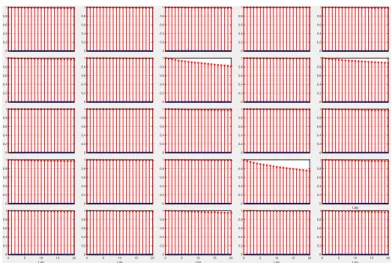
Analyzing the autocorrelation of the runs, presented in 6, we can observe that in case of simple concatenation, the coeﬃcients are around 0.4; applying the mix and overlap steps more than half this value, reducing it to bellow 0.2. We can observe that with the reduced autocorrelation, it seems that the divergence of the cumulative sum from 0 also decreases.

To statistically analyze the properties of the proposed methods, we generated 1000 sequences, each of length 10e4 for both the simple concatenation and mix and overlap. For comparison, we consider the objective ambiguity method

(10)

a) b)

0 0.2 0.4 0.6 0.8 1

0 5 10 15 200

0.2 0.4 0.6 0.8 1

0 5 10 15 200

0.2 0.4 0.6 0.8 1

0 5 10 15 200

0.2 0.4 0.6 0.8 1

0 5 10 15 20

0 0.2 0.4 0.6 0.8 1

0 5 10 15 200

0.2 0.4 0.6 0.8 1

0 5 10 15 200

0.2 0.4 0.6 0.8 1

0 5 10 15 200

0.2 0.4 0.6 0.8 1

0 5 10 15 20

0 0.2 0.4 0.6 0.8 1

0 5 10 15 200

0.2 0.4 0.6 0.8 1

0 5 10 15 200

0.2 0.4 0.6 0.8 1

0 5 10 15 200

0.2 0.4 0.6 0.8 1

0 5 10 15 20

0 0.2 0.4 0.6 0.8 1

0 5 10 15 20

Lag 0 0.2 0.4 0.6 0.8 1

0 5 10 15 20

Lag 0 0.2 0.4 0.6 0.8 1

0 5 10 15 20

Lag 0 0.2 0.4 0.6 0.8 1

0 5 10 15 20

Lag 0

0.2 0.4 0.6 0.8 1

0 5 10 15 200

0.2 0.4 0.6 0.8 1

0 5 10 15 200

0.2 0.4 0.6 0.8 1

0 5 10 15 200

0.2 0.4 0.6 0.8 1

0 5 10 15 20

0 0.2 0.4 0.6 0.8 1

0 5 10 15 20

0 0.2 0.4 0.6 0.8 1

0 5 10 15 20

0 0.2 0.4 0.6 0.8 1

0 5 10 15 20

0 0.2 0.4 0.6 0.8 1

0 5 10 15 20

0 0.2 0.4 0.6 0.8 1

0 5 10 15 200

0.2 0.4 0.6 0.8 1

0 5 10 15 200

0.2 0.4 0.6 0.8 1

0 5 10 15 200

0.2 0.4 0.6 0.8 1

0 5 10 15 20

0 0.2 0.4 0.6 0.8 1

0 5 10 15 20

Lag 0 0.2 0.4 0.6 0.8 1

0 5 10 15 20

Lag 0 0.2 0.4 0.6 0.8 1

0 5 10 15 20

Lag 0 0.2 0.4 0.6 0.8 1

0 5 10 15 20

Lag

Fig. 6.Autocorrelation coeﬃcients of the runs from fig. 5

presented in [13] as the baseline. We used the implementation¹of the ambiguity generator provided by the authors to obtain 1000 samples of length 10e4.

Fig. 7 depicts the average of the autocorrelation coeﬃcients at each lag index over the 1000 runs, for the 3 methods. The results confirm that the mix and overlap steps are highly beneficial in reducing the autocorrelation to 0.17.

Fig. 7.Comparison of the autocorrelation coeﬃcients for the tree methods.

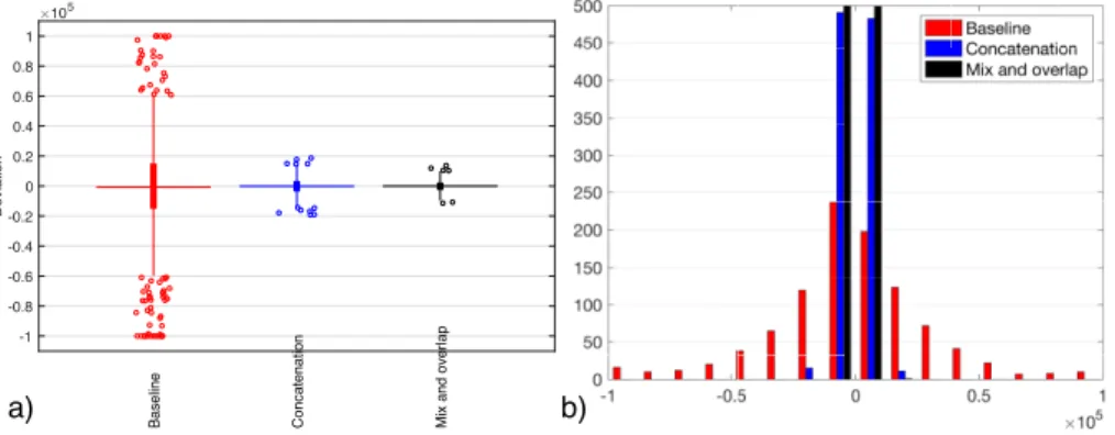
We analyzed the divergence of the methods by measuring how far is the cumulative sum from 0 at the end of sequences.The results are presented in fig.

8.

1 https://github.com/HaskellAmbiguity/AmbiguityGenerator

(11)

We can observe in fig. 8 a) too the baseline method presents many outliers, with some of the values very close to the length of the sequence, meaning that that in these runs mostly the output was all ones or all zeros.

As the proposed methods shorten these monotone runs, in order to decrease the autocorrelation, the degree of divergence in the examined timeframe also decreases, the deviation of the cumulative sums will stay closer to zero. However, as seen in the histogram in fig. 8 b), these values are still quite far away from zero, providing a good compromise between low autocorrelation and divergence.

a)

-1 -0.8 -0.6 -0.4 -0.2 0 0.2 0.4 0.6 0.8 1

Deviation

10⁵

Baseline Concatenation Mix and overlap b)

Fig. 8.Cumulative sums at the end of sequences for the three methods: a) boxplot; b) histogram.

5 Conclusions

The paper introduced a generative adversarial network model for generating data with low serial dependence. The model is used to build ambiguous binary sequences, by randomly and repeatedly combining and mixing the outputs of the network. The method is useful in setups where observes can see and record the outcome of each realization sequentially.

Empirical analysis revealed that the method provides sequences with low autocorrelation whose cumulative distribution function is non-convergent. In the long run, the method is also less likely to produce extreme departures from the half-half ratio of zeros and ones.

The study also revealed that the proposed neural network approach is not an eﬃcient building-block for generating ambiguous sequences. In order to obtain satisfactory results, many network outputs must be combined and mixed, making the method needlessly computationally expensive.

Future work will consider the development of more eﬃcient methods to obtain sequences with the same characteristics. We will also study how the length of the building-block binary samples influences the sequence’s degree of divergence.

(12)

Acknowledgments

This research was partially supported by Sapientia Foundation Institute for Scientific Research (KPI). L. Szil´agyi is J´anos Bolyai Fellow of the Hungarian Academy of Sciences.

References

1. Arl´o-Costa, H., Helzner, J.: Iterated random selection as intermediate between risk and uncertainty. In: Manuscript, Carnegie Mellon University and Columbia University. In the electronic proceedings of the 6th International Symposium on Imprecise Probability: Theories and Applications. Citeseer (2009)

2. Brock, A., Donahue, J., Simonyan, K.: Large scale gan training for high fidelity natural image synthesis. arXiv preprint arXiv:1809.11096 (2018)

3. Ellsberg, D.: Risk, ambiguity, and the savage axioms. The quarterly journal of economics pp. 643–669 (1961)

4. Gilboa, I., Schmeidler, D.: Maxmin expected utility with non-unique prior. In:

Uncertainty in Economic Theory, pp. 141–151. Routledge (2004)

5. Goodfellow, I., Pouget-Abadie, J., Mirza, M., Xu, B., Warde-Farley, D., Ozair, S., Courville, A., Bengio, Y.: Generative adversarial nets. In: Advances in neural information processing systems. pp. 2672–2680 (2014)

6. Guidolin, M., Rinaldi, F.: Ambiguity in asset pricing and portfolio choice: A review of the literature. Theory and Decision74(2), 183–217 (2013)

7. Kast, R., Lapied, A., Roubaud, D.: Modelling under ambiguity with dynamically consistent choquet random walks and choquet–brownian motions. Economic Mod- elling38, 495–503 (2014)

8. Kim, K., Kwak, M., Choi, U.J.: Investment under ambiguity and regime-switching environment. Available at SSRN 1424604 (2009)

9. Knight, F.: Risk, uncertainty and profit, kelley and millman. Inc., New York, NY (1921)

10. Ledig, C., Theis, L., Husz´ar, F., Caballero, J., Cunningham, A., Acosta, A., Aitken, A., Tejani, A., Totz, J., Wang, Z., et al.: Photo-realistic single image super- resolution using a generative adversarial network. In: Proceedings of the IEEE conference on computer vision and pattern recognition. pp. 4681–4690 (2017) 11. Riedel, F., Sass, L.: Ellsberg games. Theory and Decision76(4), 469–509 (2014) 12. Schr¨oder, D.: Investment under ambiguity with the best and worst in mind. Math-

ematics and Financial Economics4(2), 107–133 (2011)

13. Stecher, J., Shields, T., Dickhaut, J.: Generating ambiguity in the laboratory. Man- agement Science57(4), 705–712 (2011)

14. Xu, T., Zhang, P., Huang, Q., Zhang, H., Gan, Z., Huang, X., He, X.: Attngan:

Fine-grained text to image generation with attentional generative adversarial networks. In: Proceedings of the IEEE Conference on Computer Vision and Pattern Recognition. pp. 1316–1324 (2018)

15. Yu, Y., Gong, Z., Zhong, P., Shan, J.: Unsupervised representation learning with deep convolutional neural network for remote sensing images. In: International Conference on Image and Graphics. pp. 97–108. Springer (2017)

16. Zhu, J.Y., Park, T., Isola, P., Efros, A.A.: Unpaired image-to-image translation using cycle-consistent adversarial networks. In: Proceedings of the IEEE international conference on computer vision. pp. 2223–2232 (2017)