Elementary Theory of Magnetic Resonance
1 . The Physical Background
T h e historical roots of nuclear magnetic resonance spectroscopy can be traced back to the old quantum theory, which flourished during the 12-year period (1913-1925) immediately preceding the discovery of modern quantum mechanics. Indeed, the Stern-Gerlach experiment (1921)—unquestionably the precursor of all magnetic resonance experi- ments—was originally designed (7) to detect the space quantization of orbital magnetic moments; but modified versions of the experiment were later used to provide the first reliable determinations of nuclear magnetic moments. T h e experimental technique was vastly improved by the introduction of the resonance method (1938), and subsequent improvements led to precise determinations of nuclear moments by atomic and molecular-beam magnetic resonance experiments ( 2 ,3 ) . However, it was not until 1946 that nuclear magnetic resonances were detected in bulk matter (4, 5).
T h i s introductory chapter presents a qualitative discussion of the physical basis for magnetic resonance experiments and a brief account of Bloch's phenomenological theory (4). T h e relevant quantum mechan- ical theory—the theory of spin angular momentum and the quantum mechanics of magnetic moments in magnetic fields—will be discussed in Chapters 2 and 3. T h e greater part of the discussion presented in this chapter will be couched in the language of classical mechanics.
A. Angular Momentum
T h e motion of a classical point particle, relative to a suitably chosen coordinate system, is determined by Newton's laws of motion (6)
1
together with an initial specification of the position vector r and the velocity vector1
dr
v = Tt = r'
If the particle is subjected to a force field F, the position vector at any time is given by the solution of the equation of motion
F=^(mv) = p, (1.1) where m is the mass of the particle (assumed constant) and ρ = mv
its linear momentum.
For some purposes, the motion of the particle is more appropriately described in terms of the vector moments of F and p, computed with respect to the origin. The moment of force is called the torque and denoted τ; the moment of linear momentum is called the angular momentum and denoted P:
τ = r X F, P = r X mv. (1.2)
Evidently, τ is perpendicular to the instantaneous plane determined by r and F, while Ρ is perpendicular to the instantaneous plane of r and v.
An important relation between the torque and the angular momentum may be deduced by computing the vector moments of the first two members of (1.1):
_ d . . d . x
r X F = r X ^ (mv) = — (r X mv).
The last equality follows from the rule for the differentiation of a vector product and the fact that the vector product of any vector with itself vanishes identically. Thus the torque acting on a particle is equal to the time rate of change of the angular momentum:
The importance of the angular momentum in classical mechanics is based upon the fact that Ρ is a constant of the motion whenever the torque vanishes identically.2 For, according to (1.3), the vanishing of τ implies
1 H e r e , a n d subsequently, a d o t over a n y s y m b o l denotes differentiation w i t h respect to time.
2 I n general, a n y physical q u a n t i t y is said t o b e a c o n s t a n t of t h e m o t i o n if its total time derivative vanishes identically.
that Ρ is constant in magnitude and direction. Thus the plane determined by r and ν is invariable, and the motion of the particle is necessarily confined to this plane. The path traced out by the terminus of r is called the orbit, and Ρ is called the orbital angular momentum.
An example of a force field which results in the conservation of angular momentum is the so-called central force (6), where F is always collinear with r, so that r X F = 0. In the particular case of a particle whose orbit passes through the origin, conservation of angular momen- tum requires that Ρ = r X mv = 0, which implies that ν = r is collinear with r. In this circumstance, the force is proportional to r and the orbit degenerates to a straight line through the origin. In the case of a central force whose magnitude varies as the inverse square of the distance from the origin, the orbit is always a conic section.
The concept of angular momentum is of fundamental importance in quantum mechanics, but the orbital angular momentum of a quantum mechanical particle possesses properties that are remarkably different from those of a classical particle. Let Ρ denote the orbital angular momentum of a classical particle with respect to an arbitrary origin, and let η denote a unit vector specifying the direction of a variable line through the origin. If Ρ is a constant of the motion, then, according to classical mechanics, the projection of Ρ along η varies continuously from -F-1 Ρ I to — | Ρ | as the angle between η and Ρ varies continuously from 0 to π. On the other hand, the quantum mechanical theory of angular momentum asserts that a measurement of a component of angular momentum in any direction must yield some member of the sequence
-ÄL, -h(L - 1), h(L - 1), hL, (1.4) where fi is Planck's constant3 divided by 2π,
h = -^- = 1.0544 X 10⁻²⁷ erg-sec,
and L is a nonnegative integer called the orbital quantum number.
The discrete nature of the sequence (1.4) is described by saying that in quantum mechanics the angular momentum is quantized. It is con- venient to express the quantization in terms of a discrete variable Κ whose domain consists of the 2L + 1 integers: —L, — (L — 1), L — 1, L . A generic member of the sequence (1.4) is denoted fiK.
3 T h e n u m e r i c a l values of t h e f u n d a m e n t a l physical c o n s t a n t s follow t h e r e c o m m e n d a - tions of t h e I n t e r n a t i o n a l C o m m i t t e e o n W e i g h t s a n d M e a s u r e s (Natl. Bur. Std. (U.S.) Tech. News Bull., O c t . 1963).
It is important to recognize that although an experimental measure- ment of the angular momentum in a given direction η must yield one of the 2L -f 1 possible values of fiK, the probability of observing a particular value fiK' will not, in general, be unity. The probabilities of the several values of fiK are theoretically calculable (cf. Chapter 3) and, in principle, may be experimentally determined by measuring the angular momentum of a large number of identical systems S± , S2 ,
SN(N^>2L-{- 1). These experiments yield a set of TV values
fiKx , fiK2 , fiKN , where each K{ is an integer in the closed interval (— L, L). From these data one can compute the probability distribution associated with the sequence (1.4) for the direction n. If the value fiK is observed in each of the Ν experiments (i.e., the probability of fiK is unity), the direction η is called the axis of quantization.
Another distinction between the classical and quantum mechanical conceptions of orbital angular momentum is provided by the relation of the square of the maximum component of angular momentum to the square of the total angular momentum in the two theories. According to classical mechanics, the component of Ρ in a direction η is a maximum when η is parallel to P, so that (n · P)ma x = I Ρ I2· According to quantum mechanics, the square of the angular momentum is fi2L(L +1), not (/^)2 m a x = fi2L2.
The quantization of the angular momentum is a consequence of the quantum mechanical interpretation of the angular momentum as a
vector operator (cf. Chapter 2), rather than an ordinary vector composed of three scalar components. The2L + 1 quantities — fiL, —fi{L — 1), fiL
are the eigenvalues associated with the component of the angular momen- tum operator in any specified direction, and fi2L(L + 1) is the eigenvalue associated with the square of the angular momentum operator. However, the quantum mechanical properties of the orbital angular momentum approach those of a classical angular momentum in the limit as quantum mechanics approaches classical mechanics, that is, as fi —> 0. For the orbital quantum number L may, in principle, become arbitrarily large, so that it is possible for ft —> 0 and L —>• oo in such a way that the product hL remains finite. In the limit, the sequence (1.4) approaches a continuous range of values, and the square of the angular momentum
fi2L(L + 1) = WL\\ + lIL) -> fi2L2, as L -> oo.
Since the possible components of a quantum mechanical angular momentum are always integral (or half-integral) multiples of fi, and the square of the angular momentum is proportional to #2, it is convenient to introduce a dimensionless "vccior^ which ^ιπ^ευ^" the angular momentum in units of ft. In the particular case of an orbital angular momentum, this vector is denoted L, so that fiL represents the orbital
angular momentum. The component of fïL in the direction η is denoted fin · L. The eigenvalues of L2 are L(L +1); those of η · L are —L,
- ( L - 1),...,L.
B. Orbital Magnetic Moments
The quantization of orbital angular momentum requires the quantiza- tion of any physical quantity that is functionally related to the angular momentum. Perhaps the most familiar textbook example is the deduction of the quantization of the energy from the postulated quantization of orbital angular momentum in Bohr's theory of the hydrogen atom.
A second example is the quantization of the orbital magnetic moment generated by the orbital motion of a charged particle.
The relation between the orbital magnetic moment and the orbital angular momentum may be derived by considering a classical point particle of mass M and electric charge Q moving with respect to a fixed origin. The motion of the charge generates an orbital magnetic moment (7), defined by
where c is the speed of light. But the orbital angular momentum of the particle is r X Mv, so that
The scalar factor Q/2Mc is called the gyromagnetic ratio* and denoted γ.
Equation (1.6) is valid in both classical and quantum mechanics, but in the classical case it is to be interpreted as a relation between ordinary vectors, whereas in a quantum mechanical context it relates the vector operator for the orbital magnetic moment to the vector operator for the orbital angular momentum. In the case of an electron, the quantum mechanical magnetic moment operator is usually expressed in the form
t A = - 2 ^ L = ^ f l L ' ( L 7 )
where
μΒ = 9.2732 χ ΙΟ"21 ergs G"1
4 T h e electromagnetic u n i t s are gaussian cgs, so that t h e d i m e n s i o n s of γ a n d μ a r e : [γ] = rad s e c- 1 G_ 1, [μ] = ergs G- 1.
is the so-called Bohr magneton. From the quantization of L, it follows that an observation of the component of the orbital magnetic moment in any direction must yield some member of the sequence
The maximum observable component of the orbital magnetic moment operator, μΒ(Κ)ηνάχ = μΒΣ, is defined as the orbital magnetic moment of the electron. Thus an electron in a state with K = L = 1 is said to possess an orbital magnetic moment of 1 Bohr magneton. Obviously, an electron in a state with L = 0 does not generate an orbital magnetic moment.
Atomic states with L — 0 are called S states. The ground states of 1H1 and 4 7Ag1 0 7, for example, are S states.
Equation (1.6) also holds for a system of particles with charges Çi > #2 > ·-> a nd masses m1 , m2 , such that qi = kmi , where ft is a constant. The angular momentum and magnetic moment are defined as
and the condition qi = kmi shows that μ = (k/2c)P. The constant k
is just the ratio of the total charge to total mass, as one may verify by summing qi — km{ over all particles.
An analogous argument can be used to establish (1.6) for the case of a rigid body with charge density q(x, v, z) and mass density p(x, yy z) such that q(x, yy z)/p(xy y, z) is a constant. The only difference in the calculation is that summations over particles are replaced by integrations over the volume of the body.
C. The Electron Spin
The hypothesis that electrons possess an internal angular momentum was introduced into modern physics (8, 9) during the last hours of the old quantum theory (1925) to explain structural details of atomic spectra that were inexplicable on the basis of the quantization of the electronic orbital angular momentum alone. The internal angular momentum of the electron was assumed to arise from a circulation of the electronic mass brought about by an actual rotation of the electron, which was visualized as a small sphere with charge —e and mass me. Because of the evident analogy of this classical model to spinning tops, the internal angular momentum is often described as the electron spin.
In the absence of a definitive theory, the classical description of the electron spin was at best heuristic; the ultimate justification of the
—pBL, —μΒ(ί — 1), ..., μΒ^~ 1), μΒΣ.
hypothesis depended upon its agreement with experiment. I t was found that the electron-spin hypothesis was compatible with the results of experimental observations if the following conditions were satisfied:
(1) T h e component of the electron spin in any direction is of the form sfi, where s is the discrete spin variable whose range consists of two points: s = -\- \ and s = — \.
(2) T h e spin magnetic moment is related to the internal angular momentum by the equation
where fis is the quantum mechanical angular momentum of the electron.
T h e first condition demands the quantization of the internal angular momentum, but this was not an innovation in physics, since the old quantum theory had enjoyed many successes in quantizing orbital angular momentum. T h e significant aspects of the quantization were the half-integral quantum numbers and the fact that the absolute magnitude of a component of the electron spin could not exceed Ä/2.
T h e maximum value of the spin variable is called the spin or spin quantum number. Since the spin is fixed at \, fi\2 tends to zero as ft —>• 0, so that the electron spin has no analog in classical mechanics.
T h e second condition asserts that the electron gyromagnetic ratio is
—ejmec rather than — e/2mec, as might be expected from classical considerations. However, conditions (1) and (2) together imply that a measurement of a component of the magnetic moment in any direction would yield the values — μΒ for s = + · | and + / x5 for s = — \. Hence the factor of \ removed from the classical expression for the gyromagnetic ratio by (2) is replaced by (1) in an experimental determination of the electron's magnetic moment. T h u s a free electron has a magnetic moment of 1 B o h r magneton.
T h e new quantum mechanics (1926) did not include the electron spin in its theoretical structure, so that it was necessary to fit the electron spin into the theory. T h e absence of a classical model led to some difficulties (10), but eventually (1927) a satisfactory theoretical framework was developed (11) which provided a basis for the quantitative inter- pretation of the alkali doublets (spin-orbit interaction), the anomalous Zeeman effect, and the S t e r n - G e r l a c h experiment (12).
T h e theoretical problem of the electron spin was considerably clarified by the relativistic quantum mechanics of Dirac (1928). According to the special theory of relativity, the space and time coordinates must enter into the theory in a symmetrical way, whereas the (second)
Schrödinger equation prescribes that the time development of the wave function is governed by an equation that is linear only in the time derivative. The synthesis of these conditions into the principle that the space and time derivatives appear linearly in a relativistic quantum mechanics (13) requires the introduction of a new variable. The new variable was not specified initially, but upon developing the theory it turned out to be an angular momentum of spin \. The theory also predicts that a particle of mass m and charge —e possesses a spin magnetic moment with gyromagnetic ratio —ejmc.
The spin and magnetic moment of the electron are now well-estab- lished properties which are as characteristic of the electron as its mass or charge. The internal angular momentum is a property built into the electron by Nature; hence, the spin of the electron is often described as
an intrinsic angular momentum.
D. The Stern-Gerlach Experiment
The conceptual differences in the classical and quantum mechanical descriptions of angular momentum were put to a crucial test in the Stern-Gerlach experiment. This experiment provided unambiguous evidence confirming the quantization of angular momentum. At the same time, however, the experiment revealed an anomaly which was subsequently explained by the electron-spin hypothesis.
The physical basis of the Stern-Gerlach experiment rests on an elementary theorem concerning the behavior of a magnetic moment in an inhomogeneous magnetic field. Let H(x, y, z) denote a stationary external magnetic field5 and μ the magnetic moment of a microscopic physical system. In the presence of the field, the magnetic moment experiences a torque
τ = μ Χ Η , (1.9) which tends to align μ with the direction of the field at the point occupied
by μ (Fig. 1.1). The energy of orientation may be obtained from the torque-energy relation
where θ is the angle between μ and H. For a fixed, but otherwise arbitrary point in the field, it follows that
— = I τ I = μΗ sin 0, (1.10)
Ε = - μ · Η, (1.11)
5 A n external m a g n e t i c field is a field set u p in an otherwise h o m o g e n e o u s region of space w h i c h does n o t include t h e sources of t h e field. T h e curl of an external m a g n e t i c field is zero.
F I G . 1.1. T h e geometric relations b e t w e e n μ, Η , a n d τ .
where the reference level for the energy has been set at zero field. Since μ does not depend upon x9 y, or z, the force exerted on μ is given by6
-VE = ( μ · V)H
8x
(Η
dz (1.12) For the particular case where Η is a uniform field, the force vanishes and the moment does not change its position.
The Stern-Gerlach experiment is performed (Fig. 1.2) by heating a source of silver atoms in an oven Ο and allowing the thermally emitted atoms to pass from the oven into an evacuated chamber where they are collimated by slits S1 and S2 ; the atomic beam thus formed is passed through an inhomogeneous magnetic field and deposited on a plate P.
If the atoms in the beam possess a magnetic moment, by virtue of a nonvanishing angular momentum, the nature of the silver deposit will depend upon whether the angular momentum obeys classical or quantum mechanical laws.
For simplicity, let the field and its gradient be in the ζ direction, so that the force on an atom is
F d H*
F I G . 1.2. S c h e m a t i c r e p r e s e n t a t i o n of t h e S t e r n - G e r l a c h e x p e r i m e n t .
6 E q u a t i o n (1.12) follows from t h e vector identity ν(μ · Η ) = (μ · V ) H + ( Η · \7)μ + μ Χ ( V Χ Η ) + Η Χ ( V Χ μ) a n d t h e fact t h a t V Χ Η = 0 for an external field.
According to classical theory, an atom whose magnetic moment makes an angle θ with the ζ direction will be deflected an amount proportional to μζ = μ cos θ. N o w the incoming beam includes all values in the range of Θ, so that classically one expects the beam to be drawn out and deposited as a continuous band on the plate. O n the other hand, if the ζ component of the magnetic moment is a function of a discrete variable, the beam should be split into several components and deposited as discrete bands on the plate. I n the original experiment the beam was split into two components. T h e observed splitting was attributed to an orbital magnetic moment whose discrete orientations had to be an odd number, namely, 2L -f 1 , where L is an integer. I f one assumes that L = 1, and that the atoms enter the field with the most probable
velocity, measurements of yx , y2 , d> and dHzjdz permit computation of the magnetic moment. T h e original calculation showed that the observed splitting was consistent with a magnetic moment of 1 Bohr magneton.
However, if L = 1 , the theory predicts that the beam should be split into 2L -f- 1 = 3 components, corresponding to Κ = 1 , 0, — 1 . T h e two beams observed were assumed to correspond to Κ = ± 1 , but the theory was unable to account for the absence of the unperturbed (K = 0) beam.
T h e results of the Stern-Gerlach experiment are completely explained by the electron-spin hypothesis. T h e silver atom is normally in a 25 '1/2
state; that is, the resultant angular momentum is just the intrinsic spin of the 5s electron. Applying conditions (1) and (2) of Section l . C , one concludes that the beam should be split into two components with the upper and lower beams corresponding to atoms whose valence electrons are described by s = and μζ = ±μΒ .
T h e Stern-Gerlach experiment is analogous to the polarization of light waves by doubly refracting crystals. T h e direction of the magnetic field defines an axis of reference for the two independent states of spin orientation, and corresponds to the polarizer in optical experiments.
T h e gradient of the magnetic field separates the silver atoms into two groups, one with s = -f-|-, the other with s = — J , and corresponds to an optical analyzer. T h i s analogy helps to clarify the essential quantum mechanical properties of intrinsic spin angular momentum. F o r con- venience, let the beam consist of s p i n - \ particles with a positive gyromagnetic ratio. A l l particles in the upper-beam component are then described by s = + J and are said to be polarized in the positive ζ direction. I t must be emphasized, however, that the ζ direction is arbitrary. Before the beam enters the field region there is no preferred direction of quantization—the direction of quantization is established by the direction of the applied field H .
I f the magnet is rotated through an angle θ about the direction of the incoming beam, the unpolarized beam will again be split into two components corresponding to s = ± J ; but these states of quantization are referred to the new direction of the field. T h i s result emphasizes the fact that if a particle has spin J , the measurement of a component of its angular momentum in any direction can yield only ±#/2. T h e experiment is illustrated in F i g . 1.3(a), where the common direction of
F I G . 1.3. S c h e m a t i c r e p r e s e n t a t i o n s of S t e r n - G e r l a c h e x p e r i m e n t s for an u n - polarized i n c i d e n t b e a m (a), a n d ^-polarized b e a m s (b), (c), a n d (d). T h e vector A in- dicates t h e direction of t h e S t e r n - G e r l a c h analyzer.
the field and its gradient are represented by a vector A issuing from the origin of an arbitrarily chosen coordinate system. T o clarify the drawing, the beam components have be^n represented as geometric rays and the beam deposits as two points on the plate.
I f the incident beam has been selectively polarized in some direction (for example, by selecting one of the components of an initial Stern- Gerlach experiment), then the experimental results depend upon the angle θ which the direction of the polarization makes with the Stern- Gerlach analyzer A. I f θ = 0, and the incident beam consists entirely of particles with s = + \ [ F i g . 1.3(b)], then all particles in the beam are deflected in the positive ζ direction. I f the experiment is repeated with θ = π [ F i g . 1.3(c)], the beam is again deflected in the positive ζ direction.
I n this case, the Stern-Gerlach analyzer A defines a new ζ axis, and relative to this axis the beam particles all appear to be in a spin state characterized by s = — J .
F o r 0 < θ < 77, an incident ^-polarized beam will be split into two components [ F i g . 1.3(d)], but the deposits on the plate will not be of equal intensity. T h i s result is best analyzed by considering the problem
from a coordinate system whose z' axis is parallel to A. Consider first a single particle of the beam. T h e incoming particle is polarized in the ζ direction, but from the point of view of z', the particle appears to have a mixture of the -\-z and — ζ polarizations. U p o n interacting with the Stern-Gerlach analyzer, the particle exhibits one or the other of the two states of polarization, but which state of polarization will be observed for a single particle cannot be predicted. I f the experiment is repeated many times, as indeed it is with a beam, one can ask for the probabilities P+ and P_ of observing the positive or negative states of polarization.
Clearly, the intensity ratio of the two beam deposits is P+jP- and P+ + P- = 1.
T h e functional dependence of P+ and P_ on θ may be determined from the special cases already considered. W h e n ζ coincides with z\
a beam polarized in the -\-zf direction is not split by A [ F i g . 1.3(b)], so that P+ = 1 when θ = 0. W h e n θ = π, as in F i g . 1.3(c), P _ = 1.
F r o m these particular results, one can conclude that P+ = c o s2| , P_ = s i n2| .
I n optical polarization the intensities are proportional to cos2 θ and sin2 Θ;
the half angles appear in the above equations because the two independent states of polarization of a s p i n - \ particle differ in phase by 180°.
E. Nuclear Spins
T h e electron-spin hypothesis was quickly followed (1927) by the suggestion (14) that the proton also possesses an intrinsic spin angular momentum characterized by the spin quantum number \ . Somewhat surprisingly, the spin of the proton was not inferred from an analysis of the structure of spectral lines, but from the anomalous behavior of the specific heat of molecular hydrogen. O n the other hand, it had been noted by Pauli (15), before the electron-spin hypothesis, that a non- vanishing nuclear angular momentum could explain the hyperfine structure observed in atomic spectra. Pauli's suggestion referred to the angular momenta of complex nuclei which, at the time, were presumed to consist of A protons and A-Z electrons, where A and Ζ are, respec- tively, the nuclear mass and charge numbers. T h u s the proposed nuclear angular momentum did not represent an intrinsic angular momentum—the latter is an attribute of a single particle (16). However, as long as the internal structure of the nucleus is not at issue, the
distinction between the angular momenta of "simple" and complex particles is an academic one, and intrinsic is frequently used as a modifier in either case.
The first determinations of the spins of complex nuclei were based upon analyses of atomic hyperfine structure which showed that a nuclear angular momentum could be characterized as a general quantum mechanical angular momentum. In particular, the spin quantum number / may be integral or half-integral, and a component of the angular momentum in any direction is of the form nth, where m is the discrete spin variable whose range consists of 21 + 1 values:
Significant experimental results on the spins and quantum statistics of complex nuclei were obtained from studies of the band spectra of homonuclear diatomic molecules (77). In fact, the experimentally determined quantum statistics played a prominent part in the rejection of a nuclear model consisting of electrons and protons. According to quantum statistics (18), all spin-^ particles follow Fermi-Dirac statistics, and systems of spin-^ particles obey Fermi-Dirac or Bose-Einstein statistics, accordingly as the number of particles is odd or even. Experi- mentally, it was found that the statistics depended only on the mass number. On the electron-proton model, the mass number is equal to the number of protons, so that the nuclear electrons appeared to lose their identity as fermi particles. For example, 7N1 4 was found to satisfy Bose-Einstein statistics, whereas quantum statistics demands Fermi- Dirac statistics for a system of 21 fermi particles. The difficulty was resolved with the discovery of the neutron (1932). For it was immediately pointed out (19) that if the neutron is a spin-J particle, a nucleus consisting of Ζ protons and A-Z neutrons would satisfy the requirements demanded by experiment. On this model, the mass number is determined by the total number of nucléons, which in turn determines the quantum statistics.
The total angular momentum of a complex nucleus (20) is the sum of the intrinsic and orbital angular momenta of the protons and neutrons and may be written
kl = h(L + S),
where I is the dimensionless nuclear spin vector and h(L + S) denotes the sum of the orbital and spin angular momenta of the nucléons.
Since the orbital angular momentum is described by integral quantum numbers, the nuclear-spin quantum number is expected to be integral or half-integral, accordingly as A is even or odd, and this conclusion is confirmed by experiment. Furthermore, no exception has as yet
been found which violates the empirical rule that the nuclear spin is zero whenever A and Ζ are even integers. These results are illustrated in Table 1.1, which lists the spins of some common nuclei.7 It should be recognized that the nuclear spins given in Table 1.1 refer to the nuclear ground state. In excited nuclear states, the spin quantum number may be different from that observed for the ground state (20).
All subsequent references to nuclear spin will refer to the ground-state spin.
T A B L E 1.1
S P I N S A N D M A G N E T I C M O M E N T S OF S O M E C O M M O N N U C L E I N u c l e u s
>H' 1 2 2.79270
1 0.85738
5B1 0 3 1.8006
5B " 3 2 2.6880
rn2
6^
0 0
pl3 \ 0.70216
7N1 4 1 0.40357
7Ν *δ 1 - 0 . 2 8 3 0 4
9F1 9 1 2.6273
15P31 2 1.1305
F. Nuclear Moments
A nucleus with a nonvanishing spin angular momentum also possesses a magnetic moment. Indeed, it is the interaction of the nuclear moment(s) with internal and applied fields which permits the observation of effects attributed to the nuclear angular momentum.
The proton has intrinsic spin \ and one expects, according to the Dirac relativistic theory, that a measurement of the proton magnetic moment would yield an absolute value of 1 nuclear Bohr magneton,
namely,
eft
μ° = 2M~c = 5 0 0 X5 0 10~24 C r gS G _ 1'
where e and Mp are the charge and mass of the proton. Furthermore, since the neutron carries no charge, the Dirac theory predicts a zero moment for the neutron. Experimentally it is found that
μ, = 2 . 7 9 2 7 S >0, μη = - 1 . 9 1 3 0 / χ ο .
7 A co mp le te tabulation is available on request from Varian Associates, Palo A l t o , California.
These results may be expressed in terms of a dimensionless g factor by the equation
μ=gμol, (1.13)
where the components of I are m = + \ ,m = ~ \. The magnetic moment is defined as the maximum component of μ in any direction, so that£ has the values 5.58556 and —3.8260 for the proton and neutron, respectively.
Since the Dirac theory does not correctly predict the magnetic moments of the neutron or proton, it comes as no surprise to learn that the nuclear moments of complex nuclei must be determined experimentally.8 It is found that the magnetic moment can be expressed in the form (1.13), where the value of g depends upon the nucleus. Nuclear g values may be positive or negative; their absolute values usually range from 1 to 6.
If the nuclear spin is greater than \ , the absolute magnitudes of the components of μ in a given direction will range over several distinct values. The magnetic moment is defined as that component for which the spin variable has the value /:
μ =gμ0I. (1.14)
Tabulated values of the magnetic moment usually give the magnetic moment in units of the nuclear Bohr magneton, that is, μ/μ0 = gl.
However, for the description of nuclear magnetic resonance experiments it is preferable to express the relation between the magnetic moment and angular momentum vectors in terms of the nuclear gyromagnetic ratio defined by
μ = γΜ. (1.15) Comparing this relation with (1.13), it follows that
γ = $ψ. = g - J L - = 4.78948 X 10³£ rads sec"1 G"1.
The absolute values of nuclear gyromagnetic ratios usually range from 102 to 104 rads sec-1 G- 1. For example, the gyromagnetic ratio of the proton is
γρ = 2.67519 X 10⁴ rads sec"1 G"1.
8 I n this connection, it s h o u l d be n o t e d t h a t t h e D i r a c t h e o r y predicts t h a t t h e electronic g value is exactly 2, w h e r e a s t h e e x p e r i m e n t a l value is actually 2.002292.
Equation (1.15) expresses the collinearity of μ and I, but it should be pointed out that μ represents the time-averaged nuclear moment in the direction of I. That the magnetic moment is not collinear with I at all times may be made plausible by assuming that the magnetic moment is the vector sum of the orbital and spin magnetic moments. Since the neutron carries no charge, it cannot generate an orbital magnetic moment;
hence the orbital part of the assumed decomposition contains no contribution from the neutrons, and μ cannot be proportional to I.
F r o m a classical point of view (27), E q . (1.15) may be justified by noting that the magnetic moment rotates rapidly about the direction of the angular momentum. T h e time interval required for an experi- mental observation of the magnetic moment includes many periods of the rotation of μ about I, so that one observes the time-averaged value of μ in the direction of I.
A nucleus whose spin quantum number is greater than \ possesses a nuclear electric quadrupole moment which arises from a charge distribution within the nucleus that is not spherically symmetric (3).
T h e nuclear electric quadrupole moment interacts with the gradient of the electric field set up at the nuclear centroid by the surrounding electrons. T h i s interaction vanishes identically for spin- \ nuclei, and is zero for nuclei with spins / > J whenever the electronic charge distribution is spherically symmetric. Since the following chapters will be primarily concerned with s p i n - \ nuclei, the theory of the quadrupole interaction will not be considered here.
2. Classical Dynamics of Magnetic Moments in Applied Fields A. The Equation of Motion
T h e dynamics of nuclear magnetic moments in applied magnetic fields can be profitably discussed from the point of view of quantum mechanics or that of classical mechanics. T h i s somewhat paradoxical circumstance is brought about by a remarkable correspondence between the equation of motion for a classical magnetic moment and the quantum mechanical equation of motion for the magnetic moment operator. T h e precise formulation of this correspondence must be deferred to Chapter 3, but the implications of this correspondence will be anticipated in the present chapter through the frequent consideration of the nuclear magnetic moment as an ordinary classical vector. T h e particular advan- tage of this interpretation is that the solution of the classical equation of motion leads to an elegant geometric description of the resonance phenomenon.
The classical equation of motion for a magnetic moment results upon eliminating the torque and the nuclear angular momentum from the equations
μ=γΑ1, τ = μΧΗ , τ = ^ (hl).
Thus
μ = - y H Χ μ, (2.1) where μ is now interpreted as an ordinary vector.
In general, the classical motion has six degrees of freedom—three of translation and three of rotation. The three translational degrees of freedom will be removed by assuming that Η is not a function of position, although it may depend upon the time. The initial point of μ is then fixed in space, and this point will be taken as the origin.
Two additional conditions on the motion of μ may be derived from (2.1) by taking the scalar product on both sides of the equation with μ and H:
μ · μ = 0, (2.2) Η · μ = 0. (2.3) Condition (2.2) is equivalent to
4(μ·μ)=0, which may be immediately integrated to give
I μ I = μ = constant.
This result, which is valid for any time dependence of H, expresses the conservation of the magnitude of μ and reduces the problem to one with two degrees of freedom. It follows that the terminus of μ is constrained to move on the surface of a sphere of radius μ.
The second condition is not directly integrable when Η is a function of but its differential form suffices for a geometric description of the motion. Consider first the special case where Η does not change with the time, so that (2.3) is equivalent to
This equation expresses the conservation of the energy Ε = —μ · Η = constant.
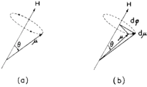
Since μ, Ε, and Η are constant, it follows that the angle between μ and Η is also constant. T h e dynamic problem is thus reduced to a single degree of freedom, so that the motion of μ consists of a rotation about the direction of Η [ F i g . 1.4(a)]. T h e sense of the rotation is
(a)
FIG. 1.4. (a) Precession of μ a b o u t t h e direction of a stationary u n i f o r m field H ; (b) t h e infinitesimal c h a n g e in μ d u r i n g a t i m e interval dt.
determined by the sign of y. F o r given any initial orientation of μ, say μ(£0), the direction i n which μ rotates, relative to the initial plane of μ(£0) and H, is determined by (2.1); hence the sense of the rotation is positive or negative, accordingly as the sign of γ is negative or positive.
T h e angular frequency of rotation about Η is, by definition, άφ
CO = —— ,
dt '
where άφ is an element of angle between successive radii on the instan- taneous circle of rotation [ F i g . 1.4(b)]. F r o m the figure it is clear that
μ S I N θ άφ = άμ = I γμ χ Η | dt;
hence
ω = I γ I Η. (2.4)
Rotational motions that evolve with time are often described as precessions, and more specifically as L a r m o r precessions if the motions are induced by the application of a magnetic field to a system of magnetic moments or moving charged particles. T h e frequency ω = \ γ \H is called the (angular) nuclear Larmor precession frequency when γ is inter- preted as the nuclear gyromagnetic ratio. I n stationary fields of the order of 10,000 G , the nuclear L a r m o r frequency is i n the megacycle range.
F o r example, the L a r m o r frequency of the proton in a field of 10,000 G is
« = y^j = 2.67519 X 10» = ^
When the applied field is a function of the time, the motion of μ is quite complicated and, excepting special cases, its analytical description cannot be expressed in terms of the elementary transcendental functions.
However, (2.4) is still valid, provided that ω and Η are interpreted as instantaneous values. Indeed, the motion of μ, over a small time interval dt, may be described as an infinitesimal rotation about the instantaneous direction of H(t). The motion of μ over a finite time interval is com- pounded from an infinite sequence of such infinitesimal rotations.
B. Integration of the Equation of Motion
An analytical description of the motion requires the integration of the system of three equations obtained from the expansion of (2.1). The integration of this system can be reduced to the integration of a single first-order equation. For this purpose, let
μ = /x(w, v, w), (2.5)
where u, v, and w are the components of a unit vector in the direction of μ. The motion of μ/μ is simply the radial projection of the motion of μ onto the unit sphere about the origin. From (2.1) and (2.5) it follows that
ù = y(Hzv — Hvzo)> ν = y(Hxw — Hzu), w = y(Hyu — Hxv). (2.6)
Now
u2 + v2 + w2 = 1, (2.7)
and this relation admits the following factorization:
(u + iv)(u — iv) = (1 + w)(l — w).
Thus one can introduce two complex parameters defined by the equations
u + iv 1 — w u +iv 1 + w I -\- w u — iv 1 — w u — iv
These parameters are not independent, since
ζ'ζ* = -1. (2.9)
The definitions (2.8), when solved for w, v9 and w, yield
u = ς _ζ > ν = - ι ^ , w = _ ζ' (2·10)
These relations identically satisfy (2.3) and (2.7), and one may readily verify that ζ and ζ' satisfy the same Riccati equation,
t = f {Hx + iHy - 2ΗΖζ - (Hx - ίΗ„)ζ*} . (2.11) T h e geometric interpretation of this reduction is simple. T h e unit
sphere about the origin is stereographically projected onto the complex ζ plane (ζ = ξ + ίη) with the south pole of the sphere as the center of the projection. T h e correspondence established by the projection is one-to-one and maps all points in the northern hemisphere onto the points of the ζ plane which lie inside the equatorial circle, while all points in the southern hemisphere are mapped onto the points of the ζ plane outside this circle. T h e north pole, for example, is mapped onto the point ζ = 0, while the south pole is mapped onto the point at infinity (ζ = GO). T h u s the path traced out by (u, v, w) is mapped onto a corresponding path in the ζ plane, and (2.11) is the equation of motion for the projected locus.
T h e geometry of the stereographic projection is shown in Figs. 1.5 and 1.6, from which one may easily deduce the projection formulas:
p 1 — w p ρ u ν I -\- zv ρ' T' ρ 1 η ' F r o m these ratios, one obtains, since ρ2, — ξ2 + η2,
F I G . 1.5. S t e r e o g r a p h i c projection of t h e F I G . 1.6. G e o m e t r y of t h e stereo- u n i t s p h e r e o n t o t h e c o m p l e x plane. g r a p h i c projection.
Hv - iH„ ) . . y2 then
y + \ί γ ί Ιζ - hI - ml i *+τ( / /*2 + H*, ) y = °- ( 2 1 7 )
If jyx and j 2 are two independent solutions of (2.17), then
l = — * ^ * k ± J & . (2.18)
ιγ(Ηχ + iHy) cxyx + ^ 2
Equation (2.18) depends only upon the ratio of the constants c1 and c2, and so contains only one arbitrary (complex) constant of integration.
The solution of (2.17) for magnetic fields that vary with time is normally a problem of some difficulty. However, in the particular case where the components of H(t) are
Hx = Ηλ cos œty Ηy = sin cot, Hz = H0 (2.19) (Άχ = ώ — ß 0 = 0), then (2.17) has constant coefficients and is easily integrated to
y = cx exp(—iQxi) + c2 exp(—iQ2t)1
If uy vy and w are expressed in terms of the polar angles ψ and #,
u = sin θ cos φ, ζ; = sin θ cos φ, zu = cos (2.13) then
ξ = cos φ tan - , ρ = tan ^ , θ θ
(2.14)
Θ γ θ
η = sin 99 tan - , ζ = elcp tan - .
Note that if ζ is the image of a point P(w, «;) = Ρ(φ) θ) on the unit sphere, the image of the diametrically opposite point P(—u, —vy —w) =
Ρ(ψ + 77, π - θ) is
= = cot | . (2-15) The solution of (2.11) can be made to depend upon the solution of a
second-order linear differential equation. For if one introduces a variable y by
Ζ7(#χ + iH2 ν y) y
where
Ω1=γΗ0Τω + [(γΗ0 Τ ω)2 + γ'Η,ψ^
Ω2=γΗ0Τω- [(γΗ0 Τ <*>ψ + γ*Ηχψ*.
From these results it is not difficult to trace back through the preceding definitions and obtain explicit expressions for the components of μ as functions of the time. A more direct method of obtaining these results will be given in Section 3 along with a geometric description of the motion.
The fields defined by (2.19) are called precessing or rotating fields,
since they rotate about the ζ axis with frequency ω and a sense of rotation given by the sign of Hy . The rotation of the full field H(i) stems from the rotation of Hxy = (Hx , Hy , 0), which is said to be circularly polarized. In magnetic resonance experiments, the frequency of Hxy is in the megacycle range, so that Hxy is frequently described as a (circularly polarized) radiofrequency (rf) field.
C. Adiabatic Change of Field
When the magnetic field is a function of t, the angle between μ and H(i) will also be a function of t. However, if the time rate of change of Η is sufficiently slow, μ will maintain a given orientation relative to H.
A simple criterion for the approximate conservation of Ζ_(μ, Η) may be obtained by examining the second derivative of μ:
μ = γ2(μ Χ Η) Χ Η + γμ Χ Η . (2.20)
The right side of this relation differs from the second derivative of μ when Η is constant, and /_(μ, Η) is rigorously conserved, only by the presence of the term γμ Χ Η. Hence the motion of μ will approximately maintain Ζ_(μ, Η) if
I μ Χ Η Κ I γ I I (μ Χ Η) Χ Η | .
Now for any vectors A and Β, | A Χ Β | < | A | | Β |, so that the above inequality will be satisfied if
I μ I I Η |< I γ I |(μ Χ Η) Χ Η | < | γ | | μ I I Η I2, or
l # K ! y l #2. (2.21)
When (2.21) is satisfied, the time rate of change of Η is said to be
adiabatic.
3. The Resonance Phenomenon A. Rotating Coordinate Systems
The classical motion of a magnetic moment in precessing fields of the form (2.19) admits a transparent geometric description when the problem is considered from a coordinate system which is initially coincident with the fixed laboratory coordinate system but subsequently rotates about the ζ axis with the same sense and frequency as the rf field (Fig. 1.7).
z'= ζ
X
F I G . 1.7. M a g n e t i c fields in t h e r o t a t i n g c o o r d i n a t e system for γ > 0 .
The motivation behind the introduction of the rotating coordinate system is that an observer in the rotating system does not observe that component of the motion generated by a uniform precession of μ about the ζ axis with the sense and frequency of the rf field. If the equation for the time dependence of μ in the rotating system can be solved, the motion of μ relative to the laboratory coordinate system is obtained by superimposing the appropriately sensed rotation about the ζ axis.
The exploitation of this idea requires a simple but important relation connecting the time derivatives of an arbitrary vector, as observed from the stationary and rotating coordinate systems. Let Κ denote a cartesian- coordinate system fixed in the laboratory, and K' a second cartesian- coordinate system whose origin is always coincident with that of Κ but rotates relative to Κ with angular velocity ω.
The angular velocity ω is measured with respect to K, and it will be assumed that observers in Κ and K' use the same system of units for
all measurements. Furthermore, differentiation with respect to the time will be denoted djdt relative to K, and δ/δ/ relative to Κ'.
If U denotes any fixed vector in K' (e.g., U could denote one of the unit vectors along the axes of K')> then, by definition
%-*
However, the vector U, being fixed in K\ rotates with angular velocity ω relative to K; hence, an observer in Κ describes the motion of U by the equation
d\J
^ Γ = ω χ υ·
Consider now a fixed vector V in the stationary system, so that
dt
An observer stationed in Κ' perceives a rotation of V with angular velocity —ω, and describes the motion of V by the equation
/ dV Λ
However, if V is a vector of Κ which is a function of time, then an observer in K' perceives not only the rotational motion —ω χ V, but also the change of V brought about by its change of orientation relative to K. Thus
S
— χ ν + £for any vector V in K.
B. Classical Description of Resonance
The application of (3.1) to the motion of a magnetic moment in an arbitrary magnetic field Η yields
| ^ r = - y J H + ^ - j x ^ (3.2)
where —yH Χ μ has been substituted for d\LJdt. All vectors in the last member of (3.2) are referred to the stationary coordinate system; the