Basic thermodynamics of electrified interfaces

1

Basic thermodynamics of electrified interfaces

Gyözö G. Láng^*

Eötvös Loránd University, Institute of Chemistry, Department of Physical Chemistry&Laboratory of Electrochemistry and Electroanalytical Chemistry

H-1117 Budapest, Pázmány P. s. 1/A, Hungary

Abstract: In this study some general aspects of the thermodynamics of systems with interfaces are discussed, and a brief treatment of interfaces within the framework of classical thermodynamics is presented. Special attention is paid to the theory of electrified interfaces.

The intensive parameter conjugate to surface area (“surface tension” or “interfacial tension”) is an important parameter also in the thermodynamic theory of electrodes, because the interactions between the adjacent bulk phases take place via interfaces, e.g. via the interface between a metal and an electrolyte solution. As a consequence, the thermodynamic properties of the interface region (i.e. the electronic conductor | ionic conductor interface) directly influence the electrochemical processes. First, to introduce the reader to the topic, basic concepts (such as

“surface”, “interface”, “interphase”, “interfacial or interface region”, “dividing surface”,

“adsorption”) are reviewed, a reasonably simple thermodynamic treatment of interfaces, together with a brief description of the models widely used in the literature, are presented, and the characteristics of the Gibbs „dividing plane” model and the Guggenheim „interphase”

model are outlined. The derivation of the electrocapillary equation, the Gibbs adsorption equation, and the Lippmann equation for an ideally polarizable electrode is given. A simple illustrative example for the application of the electrocapillary equation is presented. Some important mathematical concepts (e.g. theory of homogeneous functions and partly homogeneous functions, Euler's theorem and Legendre transformation) and various functional relationships of the thermodynamics of surfaces and interfaces are summarized.

Keywords: Adsorption, Dividing surface, Electrocapillary equation, Euler’s theorem, Gibbs adsorption equation, Gibbs dividing surface, Gibbs model, Gibbs‒Duhem equation, Guggenheim model, Homogeneous functions, Interfacial thermodynamics, Interfacial tension,

*Tel.: +36 1 209 0555/1107; fax: +36 1 372 2592.

E-mail address: langgyg@chem.elte.hu

2

Intensive parameter conjugate to surface area, Legendre transformation, Lippmann equation, Surface excess, Surface tension

Introduction and basic concepts

A “thermodynamic system” is a part of the physical world constituted by a significantly large number of particles (i.e., atoms, molecules or ions). A “homogeneous thermodynamic system” is defined as the one whose intensive thermodynamic properties are constant in space.

If a portion of a thermodynamic system behaves in this way throughout all its volume, it is called a “phase”, i.e. the term “phase” is used for a region that is chemically and structurally homogeneous. According to a more general definition, a “phase” is a region of (spatially) constant or continuously changing physical (intensive thermodynamic) and chemical properties.

A “heterogeneous system” can involve more than one phase, and the passage through the interface among two phases leads to a discontinuous variation of one or more intensive functions, such as concentrations, density, electric potential, etc.

The plane ideally marking the boundary between two phases is called the “interface”.

Although interfaces are always dealt with from a thermodynamic point of view, if attention is actually focused on only one of the two phases, the plane between the phase and the environment is called the “surface” of the phase (see e.g. [1]). The region between two phases where the properties vary between those in the bulk is the “interfacial or interface region”. It is sometimes regarded as a distinct – though not autonomous – phase and is called the

“interphase”.

The primary objectives of all thermodynamic treatments are to describe systems involving interfaces in terms of experimentally observable quantities and to derive equations (functions) that enable one to relate the thermodynamic properties of a system under one set of conditions to those valid for another set of conditions. An interface or a surface does not exist in isolation.

It is the interface region in a two-phase system and valid thermodynamic conclusions can only be drawn by considering the system, namely, the interface and the two regions adjacent to the interface, as a whole. Provided that the radius of curvature is sufficiently large, the interface/interphase may be regarded as plane and its energy then differs from that of a bulk phase by a term expressing the contribution of changes of energy due to a change of the area of contact. Edge effects can be eliminated by considering a section of an interface in a larger

3

system. There is no clear boundary between the interfacial region and the bulk of the phases so that the thickness of the interphase depends on the model chosen to describe this region.

The words “interface” and “surface” are often used synonymously, although interface is preferred for the boundary between two condensed phases and in cases where the two phases are named explicitly, e.g. the solid/gas interface [2]. Nevertheless, solid surfaces are usually not perfectly flat but are somewhat rough. The geometric area, as represented by the product of the length and breadth of a rectangle enclosing part of a surface, is not the same as the actual surface area which takes into account the areas of the hills and valleys within the rectangle. If the surface is very rough, the geometric area may be considerably smaller than the actual area. The properties of a portion of surface are dependent on orientation, and if there are many portions of different orientation, correct summation over the whole surface may be a difficult task. Such a surface is unlikely to be in a state of equilibrium and caution should be exercised when considering systems containing such surfaces. (This complication is not always dealt with in standard textbooks because they tend to concentrate on the surface thermodynamics of liquid systems which usually possess smooth surfaces.) Consideration will be restricted here to systems in which the difference between geometric and actual areas is not of major importance.

Generally, the thickness of the interface or local values of physical quantities (parameters) cannot be measured. That is the reason why integrated quantities (which are accessible experimentally, or can be calculated from experimental data) are used for the thermodynamic characterization of interfaces. Usually, these quantities are given by the expression

 

Ψ d

ββ

αα

s ^



or by

 

ξ

Ψ d

ββ

αα

s ^



where z is the coordinate perpendicular to the plane of the interface, Ψ^s is the integrated quantity, αα and ββ are the two adjacent phases, dV represents the volume element, Ξ(z) is the “local”

value (related to the area) and ξ(z) is the volume density of any extensive physical quantity in the interfacial region.

In heterogeneous systems, mobile electric charges may accumulate at the interfaces between the constituent phases, thus a thermodynamic approach requires us also to be able to characterize the state of the system containing electrified interfaces. It is obvious that heterogeneous systems with electrified interfaces can only be described by complex

4

thermodynamic models. In electrochemistry, a heterogeneous electrochemical system in which an electronic conductor phase is in contact with an ionic conductor phase is often called an

“electrode” [3-5]. Electrodes are, in fact, capillary systems, because the interactions between the different phases occur at the interface. Thus, the understanding of the thermodynamics of these interfaces is of importance to all surface scientists and electrochemists.

The aim of this brief review is to present a simple and concise treatment of electrified interfaces within the framework of classical thermodynamics, together with a brief description of the models widely used in the literature. More detailed discussions can be found in several comprehensive reviews and research papers [5-24]).

Models of the interface region

As already mentioned in the introduction, interfacial thermodynamics is the study of the application of thermodynamics to interfacial phenomena, addressing topics including adsorption, interfacial energies, interfacial tension, superficial charge, etc. and about relations between them [see e.g. 5-26]. “Adsorption” of one or more of the components, at one or more of the phase boundaries of a multicomponent, multiphase system, is said to occur if the concentrations in the interfacial layers are different from those in the adjoining bulk phases.

The concentration of a particular species varies as a function of the distance perpendicular to the surface, as shown in Figure 1a. The overall stoichiometry of the system therefore deviates from that corresponding to a reference system of (hypothetical) homogeneous bulk phases whose volumes and/or amounts are defined by suitably chosen dividing surfaces, or by a suitable algebraic method (see later).

5

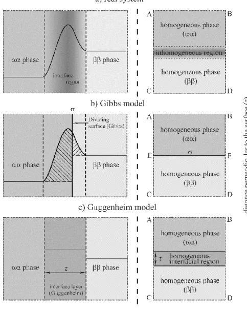
Figure 1 a) Schematic representation of the concentration profile (c_i ) of the i-th component of the system as a function of distance (z) normal to the phase boundary in the “real system” (full line);

Broken lines: boundaries of the interfacial layer;

b) Schematic representation of the concentration profile (c_i ) according to the Gibbs model of the interface; σ: the Gibbs “dividing surface” (“surface of discontinuity” or “mathematical plane”); Full line: the concentration profile (c_i ) as a function of distance (z) in the real system and in the reference system (chain-dotted lines); Broken lines: boundaries of the interfacial layer; The surface excess amount n_i^σ (or the surface excess concentration n_i^σ/A, where A is the area of the interface) corresponds to the sum of the areas of the two shaded regions of the diagram.

c) The concentration profile (c_i) according to the Guggenheim model of the interface; τ: thickness of the “interfacial layer” (“interphase”); Broken lines: boundaries of the interfacial layer;

On the right-hand sides: the macroscopic subsystems selected for investigation are represented by the ABCD rectangles.

6

Historically, there are two main approaches to describing the thermodynamic properties of interfaces. The classic work is that of Gibbs [27]; a paper by Guggenheim and Adam [28]

discusses the physical interpretation of surface excesses, and Guggenheim [29] has given a good summary of interfacial thermodynamics emphasizing a viewpoint somewhat different from that of Gibbs.

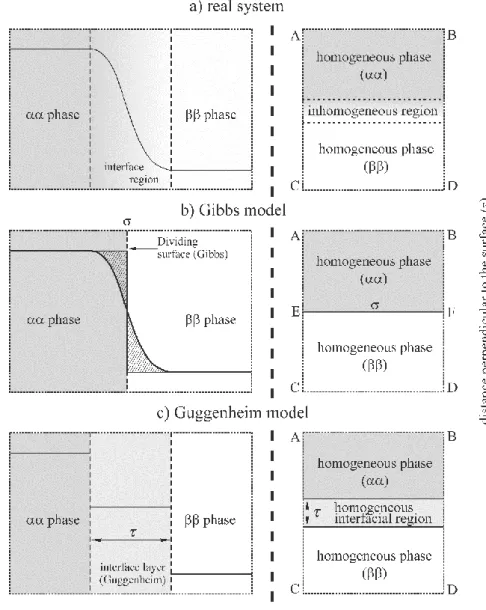
Figure 2 Schematic representation of the interfacial region. a) Real system; b) The Gibbs model of the interface; c) The Guggenheim model of the interface; On the right hand side: the macroscopic subsystems selected for investigation are represented by the ABCD rectangles.

σ is the Gibbs “dividing surface” (“surface of discontinuity” or “mathematical plane”), τ is the thickness of the “interface layer” (“interphase”);

7

As outlined above, many properties of a system vary as a function of the distance perpendicular to the surface as shown in Figure 2a (or in Figure 1a, where the concentration profile of a component is shown as a function of the position variable z). Gibbs found it mathematically convenient to consider an idealized system depicted in Figure 2b, with properties identical with those of the whole real system, that is, his approach is based on a model in which a real interface layer is replaced by a dividing surface. The “surface of discontinuity”

or “dividing surface” in the idealized system is a two-dimensional region whose position is determined by the requirements that the property under consideration should maintain a uniform value in each bulk phase right up to the dividing surface (Figures 2a and 2b). A disadvantage of this approach is that the position of the dividing surface alters according to the property considered.

In the alternative model (Guggenheim model, see Figures 1c and 2c), two dividing surfaces, one at each boundary, are employed. It is assumed that there is an “interface” or

“surface” layer of finite thickness () bounded by two appropriately chosen surfaces parallel to the phase boundary, one in each of the adjacent homogeneous bulk phases. A layer of this kind is sometimes called a Guggenheim layer, or “interphase”. A disadvantage is that terms dependent on surface volume are present in the equations, but it is difficult to assign values to these terms. (It should be noted that for very highly curved surfaces, i.e. when the radius of curvature is of the same magnitude as , the notion of a surface layer may lose its relevance.)

Given a system, subsystems consisting of a segment of the interface and finite volumes of the adjacent phases can be selected. In principle, these subsystems should not be geometrically regular in shape; however, the rectangular parallelepiped-shaped domain is usually the most expedient selection. In two dimensions, the macroscopic subsystem selected for investigation is represented by the ABCD rectangle (see Figures 1 and 2).

Let the area of the interface in the system defined according to the above concepts denoted by A, and the internal energy by U. The V volume of the system is the sum of the volumes of the two homogeneous phases  and , and the volume of the inhomogeneous (heterogeneous) region:

ββ inh

αα V V

V

V    [2]

The internal energy can be given as:

ββ inh

αα U U

U

U   [3]

etc.

8

Of course, this division is completely arbitrary, since the values on the right hand sides of equations [2] and [3] depend on the (arbitrary) choice of the dividing surface(s). In the Guggenheim model the V^ volume of the interfacial layer is

A

V^σ  [4]

The Gibbs dividing surface (or Gibbs surface) is a geometrical surface chosen parallel to the interface and used to define the volumes of the bulk phases. That is:

ββ αα V V

V   , [5]

and the volume of the “surface phase is” V^0.

Adsorption

As already discussed above, the Gibbs interface is a two-dimensional homogeneous phase without thickness (i.e. the interface is regarded as a mathematical dividing surface). In Guggenheim’s approach the interface is considered to be a 3-dimensional phase with finite thickness and volume treated in a way analogous to bulk phases, except that the thermodynamic equations contain terms related to the contributions of changes of energy due to changes of area and electrical state of the interface [5].

9

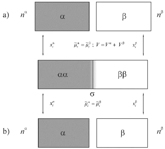
Figure 3 In the middle: the real system (an idealized surface or surface phase is separating two homogeneous bulk phases αα and ββ), and the reference systems α and β. V is the volume of the real system, V^α and V^β are the volumes of the reference phases, ~^α

μi and μ~_i^ are the electrochemical potentials, x_i^α and x_i^β are the mole fractions of component i (or constituent i) in phase α and phase β, respectively. a) Gibbs model; b) Guggenheim model.

According to these two core properties the above two (apparently different) approaches can be characterized by the following procedure:

a)There is an idealized surface or surface phase separating two homogeneous bulk phases (see Figures 1 and 2). The bulk phases are in equilibrium with the surface or surface phase.

b)Two separated reference systems  and  thought to be noninteracting homogeneous bulk phases have to be chosen (see Figure 3), the conditions of temperature, pressure, composition, etc. being identical to those in the adsorption equilibrium. Both reference phases consist of suitably defined amounts of the components. Each of the selected reference amounts is characterized by its respective molar or specific properties.

10

c) Any extensive property of the reference systems is simply the sum of the contributions from the reference amounts, without any contributions from interactions with the interfacial region in the real system.

d) The “excess thermodynamic quantities” (surface excess quantities) are the respective differences between the real system and the chosen reference systems (reference phases). The surface excess amount of component i, n_i^σ which may be negative or positive, can be defined in the Gibbs sense as the total extensive quantity minus its amount residing in hypothetical bulk phases that are uniform up to a mathematical dividing surface (“Gibbs adsorption of component i ”), or in the Guggenheim sense as an excess in the boundary zone (“surface phase”) of finite but small thickness (see equation [5]).

According to the assumptions of the Gibbs model, the reference amounts in the two reference phases are thought to be contained in and making up the volume of the actual real system, but can equally well be thought to be quite independent and spatially apart one from the other. However, it should also be noted here that from the mathematical point of view the volume of the chosen reference amounts should not be necessarily equal to the volume of the real system. (This means, that the geometric conventions employed by Gibbs in his treatment of capillary thermodynamics are replaceable by an algebraic formalism in which no mention is made of “dividing surfaces” [5,11,15,16].) It is even not necessary that the corresponding phases are effectively present in their chosen reference states within the real system. In principle, this is why the Gibbs and the Guggenheim approaches can be considered as equivalent. Nevertheless, there is an important restriction in the Guggenheim approach replacing the condition of equivalent volumes in the Gibbs method: The reference systems must be chosen in such a manner that the remaining “surface phase” has a constant thickness. Thus, this restriction essentially affects the choice of the geometrical shape of the reference systems.

However, since the reference systems are homogeneous bulk phases, their thermodynamic properties are independent of the shape. For this reason, a set of appropriate reference systems can be always selected without loss of generality. This consideration determines implicitly the selection of thermodynamic systems simply as a “section” of the interface cut out by perpendicular planes (a “parallelepiped”, a system “with cylindrical shape”, etc.) [30-34].

The surface excess amount or Gibbs adsorption of component i is n_i^ is given as

ββ β αα α β

β α α β

α σ

i i

i i i i i i i

i n n n n n x n x n n x n x

n          [6]

11

where n_i is the total amount of component i in the “real” system, x_i^ and x_i^ are the mole fractions in phases  and , respectively. n^ and n^ are the total amounts of the components (“total number of moles”) in the reference systems. From equation [6] it is obvious that the surface excess amount is well defined only when n^ and n^ are fixed. It can be also seen that with different n^ and n^ values we have different values for n_i^.

On the other hand, using the volumes of the two reference systems (V^α and V^β ) and the corresponding concentrations (c_i^α and c_i^β ), the surface excess amount of component i can also be expressed as

ββ β αα α β

β α α σ

i i

i i i

i

i n V c V c n V x V x

n       , [6a]

or, according to the Gibbs model if c_i is the concentration of species i in a volume element dV, then

  _  





surface Gibbs to

ββup phase

ββ

surface Gibbs to

ααup phase

αα

σ c c dV c c dV

n_{i i i i i} .

[6b]

The total surface excess amount of adsorbed substance, n^σ is





i σ i

σ n

n . [7]

According to the above rules the surface excess X^ of any extensive property X is calculated as

β α

σ X X X

X    , [8]

where X denotes the value of the extensive property in the whole system, X^αand X^β are the values in the reference systems.

The relation that gives the internal energy U as a function of the extensive parameters is a fundamental relation. If the fundamental relation of a particular system is known, all conceivable thermodynamic information about this system can be ascertained [35].

The internal energies of the reference phases are given by





α α α

α U S ,V ,n n_m

U   [9a]

and

12





β β β

β U S ,V ,n n_m

U   [9b]

The internal energy (U ) of the system depends on the entropy (S ), volume (V ), the amounts n₁ ... n_m of the components 1 ... m, and the surface area (A), respectively:





U

U , , , ₁ . [10]

The excess of the internal energy is given by

β α

σ U U U

U    , [11]

and the excess of the entropy is

β α

σ S S S

S    . [12]

The excess internal energy function





σ σ σ

σ U S ,V ,A,n n_m

U   [13]

is a homogeneous function of degree one with respect to all variables (see Appendix I), if V ^  0 (Gibbs model), or V ^ = A (Guggenheim model), since under these conditions









σ kS ,kV ,kA,kn_i kn_m kU S ,V ,A,n_i n_m

U    [14]

for all k > 0 real numbers. Therefore, in the framework of the Gibbs model:

σ σ σ

σ σ

i i

in γA

S T

U ^{  }



where γ is the intensive (interfacial) parameter conjugate to the extensive variable A.

Equation [15] follows from Euler’s theorem for homogeneous functions (Appendix II), i.e. it is a simple mathematical consequence of the homogeneous degree one property of the excess internal energy function [5,36].

For a system in thermodynamic equilibrium

T T T T T

T^σ  ^α ^β ^αα ^ββ , [16]

and

i i i i i

i     

^σ  ^α  ^β  ^αα ^ββ , [17]

13

etc. This means that is not necessary to use superscripts to distinguish T, ₁ … _m, in the different equilibrium phases because these must have uniform values throughout , , , 

and  (due to the equilibrium assumptions).

In the two reference phases the following relationships are valid:

α α

α α

i i

in pV

TS

U ^{  }



and

β β

β β

i i

in pV

TS

U ^{  }



According to equation [15] γ is defined by

σ σ 1 σ, σ

nm

n

A S

γ U





 







  [19]

Although this expression is mathematically correct, it is not really useful for practical purposes.

Equation [15] expresses the dependence of the excess internal energy on the variables S^σ, A, n₁^σ

… n_m^σ . This set of independent variables is not by any means the most convenient. It is usually preferable to use T as an independent variable instead of S. If the experiment is such that the external conditions are constant temperature and constant pressure, the most convenient potential function to use is the Gibbs free energy function, G(T,p,n₁ … n_m), obtained from U(S,V, n₁ … n_m) by two subsequent Legendre transformations (Appendix III):

α α α

α U pV TS

G    [20a]

and







U pV TS

G . [20b]

Consequently:

α α

i i

in

G ^



and

14

β β

i i

in

G ^



The excess Gibbs free energy function is given as

σ σ

i i

in γA

G ^{ }



and γ is defined by

σ σ

,1

σ

nm

n

A T

γ G





 







  . [23]

Unfortunately, this definition of γ is still not appropriate for experimental studies or to confirm experimental results since G^σ(T,A, n₁^σ … n_m^σ ) remains ill-defined and arbitrary (because n₁^σ … n_m^σ clearly depend on the selection of the reference systems). The Gibbs free energy function for the whole system can be expressed as:

 













i

i i i i i

i i i

i i i

i

in μn μn γA μ n n n

μ

G γA ^{α β σ α β σ} . [24]

Equation [24] indicates that γ can also be defined in terms of the Gibbs free energy function of the whole system as

nm

n p

A T

γ G

1 , ,



 







  . [25]

or in terms of the Helmholtz (free) energy function as

nm

n V

A T

γ F

1 , , H



 







  . [26]

(The Helmholtz energy or “free energy” function is defined as the Legendre transform of the internal energy function (F_H = U – T·S ).) On the other hand ‒ still remaining in the framework of the Gibbs model ‒ it should be noted, that since no volume term appears in equation [15]

there is no distinction between the surface Helmholtz and Gibbs free energies.

According to the above discussions, G^ is a partly homogeneous function of degree one in the variables A and n₁^σ … n_m^σ . The expression for the total differential of G^ is

15

σ , σ σ

σ

σ d d d

d

σ σ

σ 1 σ

σ 1

i

i T,An

n T,n n

A,n

A n A G

A T G

T G G

i j m

m







 







 



 







 



 







 





. [27]

Taking into account that

 

 



 







 S

T G

nm

A,n1^{σ σ}

σ



, γ

A G

nm

T,n

 



 









σ σ 1

σ



, and _i

n T,A ji

A

G  

 









σ

, σ

, equation [27] can be written as:

σ σ

σ d d d

d _i

i

i n

γ A T S

G ^{  }



We can get another expression for dG^σ by taking the differential of equation [22] :











i

i i i

i

i n n

A γ γ A

G d d d d

d ^{σ σ σ} [29]

There are thus two (general) expressions for dG^ (equations [28] and [29]), both of which are correct [5,36]. This can only be the case if

0 d d

d ^σ

σ  



i

i

ni

A γ T

S  . [30]

Equation [30] is the so-called Gibbs-Duhem equation for interfaces.

At constant temperature:







i

i

ni

Adγ ^σd . [31]

Dividing both sides of equation [31] by A yields









i

i i i

i

i Γ

A

γ n d d

d

σ

[32]

where Γ_i is the surface excess concentration of species i. Equation [32] is commonly called the Gibbs adsorption equation.

In the case of liquid/liquid interfaces the interfacial intensive parameter (γ) can be identified with the “interfacial tension” or “surface tension”. (Note that in case of solid/liquid interfaces there is some controversy in the literature concerning the correct name and meaning of γ [5,23,24,30,37,38].)

16 Two remarks on equation [32] are in order here:

1. First, in the case of ionic components (charged species, electrified interface)

“electrochemical potentials” (μ~

i) may be used instead of “chemical potentials” in the corresponding equations.

2. It follows from Equation [6] (which is the definition equation of the surface excess amounts) that the Γ_i values are uncertain, since they depend on the arbitrary selection of n^ and n^. However, for comparison of model predictions with experimental observations experimentally determinable (“measurable”) physical quantities are required that do not depend on the size of the reference phases.

The following procedure can be used for this purpose:

At constant T and p the Gibbs-Duhem relationships for the two reference bulk phases are 0

αd 



i

xi  _[33a]

and

0

βd 



i

xi  _{. [33b]}

Using the above two relationships it is possible to express d₁ and d₂ (i.e. the differential changes of the chemical potentials of two selected components) as a function of the other di values and the mole fractions at constant temperature and pressure

i i

i

x x x

x  

 d d

d

1,2 α 1

α α 2

1 α 2

1









 . [34a]

and

i i

i

x x x

x  

 d d

d

1,2 β 2 β β 1

2 β 1

2









 . [34b]

Combining equations [32],[34a] and [34b] and by taking into account that





1

i i i

i n n x n x

Γ  A   [35]

17 we obtain

i i

i i i

i

i x x x x

x x x n x x x x x

x x x n x A n

γ 1 d

d

1,2

β 1 α 2 β 2 α 1

β α 1 α β 1 β 2

1 α 2 β 2 α 1

α β 2 β α 2



 

 







 



 



 [36]

or

i i

i i

i i

i x x x x

x x x Γ x x x x x

x x x Γ x Γ

γ d

d

1,2

β 1 α 2 β 2 α 1

β α 1 α β 1 β 2

1 α 2 β 2 α 1

α β 2 β α 2



 

 







 



 



 . [37]

Equation [37] can be written in the simpler form:

i

Γi

γ d

d

1,2 i







 , [38]

where Γ_i^' denotes the (relative) surface excess of component i with respect to the two selected components. It is obvious from equations [36] and [37] that the Γ_i^' values do not depend on the selection of the reference systems (that is, on the selection of n^ and n^). As a consequence of the above equations, the Γ_i^' values can be determined from experimental data according to the following formula:

i j i

j i T pa

p i T

i a

γ RT Γ γ







 







 

 



 







 



, , ,

, '

ln 1

  ^[39]

(or more exactly

   

i j i

j ii T pa

i μ i

i a

γ μ RT

Γ γ



















 

 











 





1,2 1,2 , ,

'

ln 1

d ), where a_i denotes the relative

activity of component i.

Equation [38] (the Gibbs adsorption isotherm or also called the Gibbs adsorption equation) is one of the most important results from interfacial thermodynamics and it is used all the time in physical chemistry and surface science.

The electrocapillary equation

When dealing with heterogeneous electrochemical systems containing electrified interfaces the expressions derived above should be modified. In such systems, the “electrode”

is a typical basic unit. The term "electrode" is used here to denote heterogeneous electrochemical systems, in which at least two phases are connected and one of them is an

18

electronic conductor or a semiconductor, the other is an ionic conductor, usually an electrolyte solution.

In case of an electronic conductor (metal)/electrolyte solution interface we should take into account that the solvent of the electrolyte solution is not a component of the electronic conductor or semiconductor phase. The same may be true for other components. Let  denote an ionic conductor phase (e.g. an aqueous electrolyte solution) and let  denote the electronic conductor (or semi-conductor) phase. In the electrolyte solution component 1 (the “solvent” S) is e.g. water (or another component which is absent from the electronic conductor phase). We denote the mole fraction of this component by x_S^α , and therefore

α S α

1 x

x  . [40]

and

β 0

S β

1 x 

x . [41]

On the other hand, we can select a component (constituent) M of the metal phase (component 2), which is absent from the electrolyte solution, i.e.

β M β

2 x

x  [42]

and

α 0

M α

2 x 

x . [43]

We can consider that in the metal phase there is a formal electrochemical (“dissociation”) equilibrium between atoms of metal M_i and the corresponding cations M_i^zi of ionic charge z_i and the electrons e^– (i.e. we can consider these species as constituents of the metal phase). The condition of electroneutrality can be temporally relaxed, so, all the extensive variables appearing in equation [38] may be treated as independent. The electron is the only component besides metal ions in a pure metal phase. Of course, in case of alloys we have several components. According to the above equation [38] can be rewritten as

i i

i i

i x

Γ x x Γ x Γ

γ d^~

d

1,2

β M

β α M

S α



 



 



  



 . [43]

For “ideally polarizable” electrodes:

19

k k k

j j

j x

Γ x x Γ

Γ x Γ

γ d~ d^~

d

M M S

S







 



 

 











 



 , [44]

where index j denotes components in the electrolyte solution (phase α), index k refers to components of the metal phase (phase β). (The term “ideally polarizable interface” is used when no charged component is common to both phases adjoining the (electrified) interface.

Heterogeneous electrochemical systems that possess this property are called “ideally polarizable” or “ideal polarized” electrodes. The concept of ideal polarizability implies the total absence of charge transfer between the two adjacent phases.)

Electrocapillary measurements, like any other electrochemical measurements, require the use of a complete cell containing (at least) two electrodes. In a two-electrode cell one electrode is the ideal polarized electrode; the other electrode is a reversible charge-transfer electrode, which is reversible (in the Nernstian sense) to one of the ions of the solution. This second electrode of the electrocapillary cell is called the indicator electrode and is usually denoted by the symbol IN. The particular ion of the solution to which electrode IN is reversible will be called the indicator ion. An electrolyte solution containing c cationic species and a anionic species could be prepared in many different ways. However, a general electrocapillary equation can be derived if we assume that the ions of the solution are furnished by neutral binary salts [5,10,13]. Of the c × a different binary salts that could be chosen, we shall select c + a – 1 binary salts in the following way: If the indicator electrode IN is reversible to cation j’, we arbitrarily select an anion, say k’. If the indicator electrode is reversible to anion k’, we arbitrarily select a cation, say j’. In either case we have selected a binary salt containing ions j’

and k’. We call this salt the indicator salt. The electrolyte solution is then considered to have been made up by dissolving c + a – 2 additional binary salts of which c – 1 have anion k’ in common with the indicator salt; the remaining a – 1 salts have cation j’ in common with the indicator salt [5,10,13]. Thus the Gibbs adsorption equation for an ideally polarizable electrode and for the cation-reversible indicator electrode at constant temperature T and pressure p can be given in the following form [5,13,28,39]:

 

j j

j h j k

j k k j h k h

h

h h h

k j k

k

k j h k k

j j

j

k j h j i

i

i i i

Γ z Γ z

Γ

Γ Γ

Γ E

γ q







 













 























 



















































 















1 d d

d d

d d

d _M

, [45]

20

where γ is the interfacial intensive parameter, q_M is the charge density on the metal side of the interface, E₊ is the electrode potential with respect to the cation-reversible indicator electrode, subscript i indicates the components (metals) in the metallic phase (a single phase alloy), subscript h designates the neutral molecular species in the solution, the z-s are the ionic charges, the Γ and μ values are the surface excesses and chemical potentials of the various components, respectively, and the  -s indicate the number of moles of cations (or anions) per formula weight of the salt.

The above equation or more generally, the equation

 

j j

j h j k

j k k

j h k h

h

h h h

k j k

k

k j h k k

j j

j

k j h j i

i

i i i

Γ z Γ z

Γ

Γ Γ

Γ E

q T γ s





 

 













 



 









 







 

 





















































 













 1 d d

d d

d d

d

d ^σ _M

[46]

is usually called the “electrocapillary equation”. Equations [45] and [46] can sometimes be written in somewhat simpler forms [1]. However, even in the case of a very simple system the Gibbs adsorption equation could take various forms depending on the choice of independent components, the indicator electrolyte and the indicator ion.

From equations [45] and [46]

M , , ,

γ q

k

T j

p

 



 







 



  ^{, [47]}

where

k k

k j

j

jΓ F z Γ

z F

q^{M }





Equation [47] is usually called the Lippmann equation [1,5,13,39].

A simple illustrative example for the application of the electrocapillary equation

We consider a planar interface between two homogeneous phases. The phase β is supposed to be a pure liquid metal (e.g. mercury) thought to dissociate into metal ions M⁺ and electrons e^–. Let phase  be an electrolyte solution with cations K⁺ and anions A^– (originating from the dissolved salt, KA) in a not dissociated solvent L. Let the interface between the two phases be. The amounts of a component i in the two bulk phases and in the interphase are n_i^,

21

n_i^ and n_i^σ, and the (total) chemical amounts of M⁺, e^–, K⁺ and A^– in the whole system are n_K+ , n_A– , n_M+ , n_e–, respectively.

The total differential of the (excess) internal energy of the interface is

σ σ σ

σ d d ~ d

d _i

i

i n

γ A S T

U ^{  }



with the intensive interfacial parameter γ. The Gibbs–Duhem equation can be written as

~ 0 d d

d ^{σ σ}

σ  



i

i

ni

γ A T

S  , [50]

Electroneutrality in the bulk phases and in the whole system corresponds to

α A α K^ x ^

x , [51a]

β e β M^ x^

x , [51b]

and

e 0

M A

K n  n  n 

n . [52]

The excess amounts in the interface can be calculated with the help of the following material balance equations:

β M β M M σ

M^ n ^ x ^n ^

n [53a]

β e β e e σ

e^ n^ x^n^

n [53b]

α K α K K σ

K^ n ^ x ^n ^

n [54a]

α A α A A σ

A^ n ^ x ^n ^

n [54b]

α L α L L σ

L n x n

n   [55]

At constant temperature the Gibbs adsorption equation can be written as:

~ 0

~ d d

~ d

~ d d

d ^σ

e σ e σ M σ M σ L σ L σ A σ A σ K σ

K     

n    n    n  n    n 

γ

A [56]

22

In (electro)chemical equilibrium, the electrochemical potentials ~_^ _^zF^ are constant across the system for each species (F is the Faraday constant, the superscript indicates the corresponding phase). Consequently

α α

K α K σ K K

~

~

~    

        F [57]

α α

A α A σ A A

~

~

~    

        F [58]

α L σ L

L  

   [59]

β β

M β M σ M M

~

~

~    

        F [60]

β β

e β e σ e e

~

~

~    

       F [61]

σ KA A KA

K A K

~

~     

          . [62]

The Gibbs–Duhem equations for the bulk phases at constant T and p have the following forms:

0

~ d

~ d

d ^α _L^α _L^α

A α A α K α

K  n   n μ 

n   [63]

~ 0

~ d

d ^β

e β e β M β

M   n   

n [64]

From equations [50]–[64] one obtains

   











     









 



   



 β α β

e A KA K

α L L α K

K d d~ d

d 1 n  n n  F  

x n x

γ A . [65]

The change in the potential difference between the two phases can only be measured in an electrochemical cell containing a reference electrode. If the reference electrode is reversible with respect to the anion A^–, the change in the (measurable) electrode potential can be expressed as



 



d  1       

F ^. [66]

Combining equation [65] with equation [66], we find after some algebra,