Interactive Rendering Framework for Distance Function Representations
Csaba Bálint, Gábor Valasek
Eötvös Loránd University csabix.balint@gmail.com
valasek@inf.elte.hu
Submitted March 5, 2018 — Accepted September 13, 2018
Abstract
Sphere tracing, introduced by Hart in [5], is an efficient method to find ray- surface intersections, provided the surface is represented by a signed distance function (SDF) or a lower estimate of it.
This paper presents an interactive rendering framework for visualising ex- act and estimate SDF representations. We demonstrate the performance of the system by visualising 3D fractals and its modularity by rendering alge- braic and meta surfaces. In addition, we discuss SDF estimation of algebraic surfaces.
Keywords: Computer Graphics, Signed Distance Functions, Real-time Ren- dering
MSC:65D18, 68U05
1. Introduction
Rendering surfaces represented by signed distance functions (SDF) has not been in the spotlight of computer graphics research. Even though fractals have been a focus of much interest on on-line forums, literature on rendering a more general representation of surfaces, namely direct visualisation of SDFs, is scarce; the latest advancement in the field is the contribution of Keinert et. al. in [6] (2014).
A general SDF rendering engine has a far greater flexibility than incremental image synthesis based systems; even ray-tracers of practice are limited to a fixed set of surface approximations. In an SDF based rendering engine, CSG1-models, 3D
http://ami.uni-eszterhazy.hu
5
fractals, algebraic surfaces, and meta-surfaces can all be rendered directly without any pre-processing. This means that the surfaces appear in a considerably higher quality than any pre-processed polygon approximation.
However, the main disadvantage of using SDFs is the lower rendering speed compared to incremental image synthesis based rendering engines. Additionally, traditional ray-tracers and game engines both use the same set of primitives (usually polygons) which does not include SDFs. This paper focuses on the representation and rendering of SDFs, with emphasis on the case of algebraic surfaces.
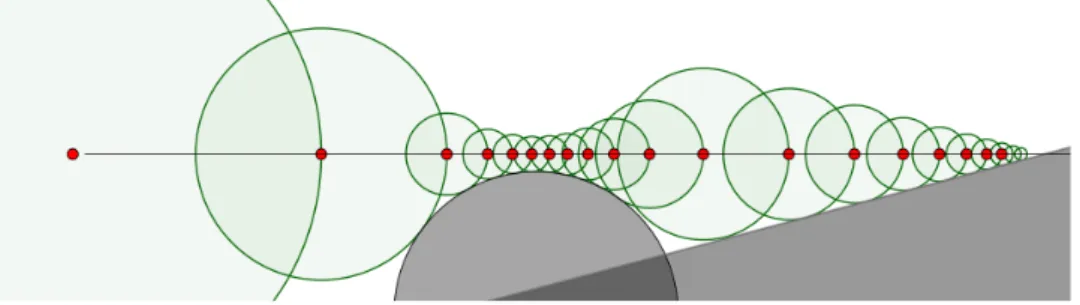
Previous work The algorithm for rendering SDFs known as sphere-tracing was first investigated by Hart in [5] (1994). It is an iterative ray-tracing algorithm, illustrated in Figure 1. This algorithm has been commonly used for the past two decades for rendering SDFs, most notably fractals [3, 4, 7, 9].
Figure 1: Illustration of the sphere-tracing algorithm in 2D.
At every point (red dot) along the ray, the distance to the surface is estimated, in this case, to the union of a half-plane and a circle. This distance defines a sphere (green circles) in which there are no intersections between the ray and the surface. Thus, sphere-tracing travels this distance
along the ray to get the next estimate of the intersection point.
Following a short overview of singed distance functions, we introduce an al- gorithm for algebraic surface visualization. Approximating the surface normal is common problem, for witch a novel method is presented in Section 5.
2. Signed Distance Functions
In this section, definitions and notations are introduced for future reference. Defi- nition 2.2 is from Hart’s original work in [5].
Definition 2.1(Distance to set). Let(X, d)be a metric space,x∈X, andA⊂X.
Then let d(x, A) := infa∈Ad(x, a) (whereinf∅:= +∞).
Definition 2.2 ((Signed) Distance Function). The f : Rn → R function is an exact (singed) distance function, or (S)DF, if for anyppp∈Rn:
1CSG, Constructive Solid Geometry: A tree-like representation of the scene using primitive objects as leaves, set operations as nodes, and transformations as edges. [2]
f(ppp) =d ppp, f−1(0)
or f(ppp) =
(d(ppp,bound(D)) if ppp∈D
−d(ppp,bound(D)) if ppp6∈D
!
. (2.1) Where bound(D) =D\int(D)denotes the boundary of a set.
Definition 2.3 (Distance Function Estimate). The f : Rn → R function is a (signed) distance function estimation if and only if there exists a q:Rn →[1, K) bounded (K∈R) function, such thatf·q is a (singed) distance function.
Remark 2.4. Besides the SDF being an upper bound to the estimate, Definition 2.3 provides a lower bound for the estimate, so sphere-tracing algorithms still converge.
The following theorem by Hart [5] describes how SDFs representing objects can be combined to create more complex geometries using CSG-like constructions.
Figure 2a shows an application of the polynomial soft-min/max versions of set operations to various geometries.
Theorem 2.5 (Set operations). Let f, g∈Rn→Rbe (S)DF. Then
(i){f ≡0} ∪ {g≡0}={min(f, g)≡0}, (ii){f ≡0} ∩ {g≡0}={max(f, g)≡0}, (iii) {f ≡ 0} \ {g ≡ 0} = {max(f,−g) ≡ 0}. Additionally, the min(f, g) and max(f, g)are (singed) distance function estimates.
(a)Soft-min/max using 3 tori, 3 cylinders, 2
spheres, 1 cube, and 1 plane (b) Meta-surface of 2 spheres, 1 cube, 1 torus, and 1 plane
Figure 2: Demonstration of the CSG model capabilities using our rendering engine Moreover, by using different blending functions between primitive geometries one can achieve the look of different phenomena, like water [8]. Figure 2b shows meta surfaces rendered in our system.
3. Algebraic surface estimation
Let us now consider the problem of estimating SDFs to algebraic surfaces of the form f(x, y, z) =
ni
X
i=0 nj
X
j=0 nk
X
k=0
aijkxiyjzk (aijk∈R). To construct an SDF from this, we have to use the following theorem [5]
Theorem 3.1. Iff∈Rn→Ris a (S)DF, it is Lipschitz continuous, andLipf = 1. Therefore, for any Lipschitz continuous f function Lipff is a signed distance function estimate. Although algebraic surfaces are not Lipschitz continuous over R3, they become Lipschitz over any finite bounded subset of space. In this case, if the distance from a given point to the surface is r, the estimation would be f(ppp)/Lipf|Sr(ppp) =f(ppp)/LipSr(ppp)f , where Sr(ppp)is the sphere with centreppp and radiusr >0. This provides the following fixpoint-iteration
F(r, ppp) = f(ppp)
LipSr(ppp)f =r. (3.1) IteratingFon its first argument,r, results in an estimation of the distance function.
Usually, we have to calculate the distance in a certain direction, for example along a ray. Letsss(t) :=ppp+t·vvv. We must calculate the Lipschitz constant of the following on a given Sr(ppp)set.
f(sss(t)) =
ni
X
i=0 nj
X
j=0 nk
X
k=0
aijk(px+tvx)i(py+tvy)j(pz+tvz)k (3.2) The substitution method for calculatingLip[−r,r]f◦sssof (3.2) is treating this expression as a f ◦sss ∈ R[t, px, py, pz, vx, vy, vz] seven variable polynomial. Mul- tiplying out, then ordering the terms, we get N ≤ ni+nj+nk + 1 number of monomials in t. LetPn(ppp, vvv)·tn denote thenth monomial.
Therefore, Lip
t∈[−r,r]
(Pn(ppp, vvv)·tn)≤n·rn−1|Pn(ppp, vvv)|is the estimate of the Lips- chitz constant of thenth monomial2, where ris from (3.1), and the sum of these is the upper-estimate of the Lipschitz constant off.
The problem with this approach is that in practice, we have to be able to make symbolic calculations within the engine and generate GPU code based on the algebraic surface given.
4. Taylor-series method
Our method is based on the fact that a Taylor expansion of a polynomial is itself.
To calculate Pn(ppp, vvv) first we note that Pn = n!1(f ◦s)(n)(0). Now, let us find an efficient way to compute the nth derivative off ◦sss. Let
gijk(t) := (px+tvx)i(py+tvy)j(pz+tvz)k (t∈[−r, r]), (4.1) so Pn=
ni
X
i=0 nj
X
j=0 nk
X
k=0
aijk
g(n)ijk(0)
n! . Lethijk(t) := ivx
px+tvx
+ jvy
py+tvy
+ kvz
pz+tvz. Note thatg0ijk=gijk·hijk, sog(n+1)ijk =
Xn
m=0
n m
gijk(m)h(n−m)ijk , where
2On estimating Lipschitz constants: [1]
h(n)ijk(t) = (−1)n·n!
"
i px
vx
+t −n−1
+j py
vy
+t −n−1
+k pz
vz
+t −n−1#
. (4.2) Thus,h(n)ijk, g(n)ijk, andPn can all be computed, and so is the following approxima- tion:
Lip
[−r,r]
(f◦sss) = Lip
t∈[−r,r]
ni+nj+nk
X
n=0
Pn·tn
!
≤ XN
n=1
n·rn−1|Pn|. (4.3) Finally, repeating the (3.1) iteration gives us the distance estimate.
Algorithm 1:CalculatingPn
In : ppp, vvvandfin sparce-form:
f(x, y, z) =PL
l=0Al·xIl yJl zKl whereA∈RL;I, J, K∈NL Out :P∈RNis forPncoefficients.
Temp :G, H∈RNforgijkandhijk. P:= (f(ppp),0,0, ...,0);
forl= 0.. L−1do G:=
pIlx ·pJly ·pKlz ,0,0, ...,0
; forn= 1.. N−1do
Hn−1 :=−(−1)n(n−1)!· Ilvnx
pnx +Jlvny pny +Klvnz
pnz
!
; form= 0.. n−1do
Gn:=Gn+n−1 m
·GmHn−m−1;
Pn:=Pn+ 1n!Al·Gn;
Algorithm 2:Fix-point iter- ation
In : The rayppp, vvv∈R3, andP∈RN coefficient vector from Algorithm 1 is given. For better convergence, aλ∈(0,1]relaxation constant, andr0>0starting radius, eg.
from linear approximation, is also given.
Out :r >0distance that can be travelled along the s
s
s(t) =ppp+t·vvv (t >0)ray.
Temp :The Lipschitz constants will be calculated inLip >0variable.
r:=r0;
fori= 0.. itersdo Lip:= 0;
forn= 1.. Ndo
Lip:=Lip+n·rn−1|Pn|;
r:=r·(1−λ) +f(ppp) Lip ·λ;
Figure 3: Novel algorithms for algebraic surface visualization.
First, using equations (4.1)–(4.3), thePncoefficients of the Taylor expansion off◦sssare calculated.
Second, the fix-point iteration in (3.1) is used to find the right step size for the sphere-tracing algorithm.
Implementing this approach is easier as it does not require symbolic expres- sions and complex code generation, see the algorithms on Figure 3. Figure 4 sum- marises our results. The algorithm can be stopped at any derivative thus achieving quadratic complexity in the number of derivatives and linear in the number of terms.
Figure 4: Comparison of SDF estimations with capped amount of steps along a ray.
The algebraic surfacefK1,K2(x, y, z) = (x2+y2+z2)(K1x2+K2y2)−2z(x2+y2) = 0has a singular line that makes it hard to visualize from this angle. The Taylor method converges closer to the surface in less steps in about the same time as the traditional linear and quadratic SDF approximations. The
light-blue means it only takes one step, and in the red region it takes 70.
5. Normal estimation
The surface normal atppp∈ {f ≡0}is defined as the unit vectornormnormnorm(ppp) = k∇∇f(pf(ppp)pp)k2, for any surface defined by the differentiable implicit functionf ∈R3→R.
In this section, we focus on calculating the normal numerically. The one-sided (forward or backward) difference method gives an error ofO()for the derivative.
A more accurate method is the symmetric difference:
∇f(x, y, z) = 1 2·
f(x+, y, z)−f(x−, y, z) f(x, y+, z)−f(x, y−, z) f(x, y, z+)−f(x, y, z−)
+O 2
. (5.1)
The idea of our approach is to take the following vectors (or stencil) vvv1:= [+1,0,0]>, vvv3:= [0,+1,0]>, vvv5:= [0,0,+1]>, vvv2:= [−1,0,0]>, vvv4:= [0,−1,0]>, vvv6:= [0,0,−1]>, then (5.1) is equivalent to∇f(ppp) = 21 P6
i=1f(ppp+·vvvi)·vvvi, thus we define normnormnorm(ppp) = 1
Z X6
i=1
f(ppp+·vvvi)·vvvi . (5.2) where Z ∈ R is the normalising constant. This means that the samples of the function are taken at the vertices of an octahedron.
(a)Error in relation to. Line breaks when the angle between the analytic and the numeric estimation is zero.
mean median one-sided 119 562
tetrah. 113 843
octah. 1.0 1.0
cube 0.6 0.7
icosah. 0.5 0.1 dodecah. 0.5 0.1
std max
one-sided 382 306 tetrah. 265 313
octah. 1.0 1.0
cube 0.5 0.6
icosah. 0.4 0.3 dodecah. 0.4 0.3 (b) Relative error to symmet-
ric difference for= 0.01
Figure 5: Error of normal estimators measured in cosine distance3.
Our tetrahedron kernel performs slightly better than the one-sided approach and results in a marginally lower mean error with lower variance. Cube, icosahedron and dodecahedron kernels also slightly out-
performed the symmetric difference, but they also take considerably more samples.
According to our measurements, an optimal stencil vector set would consist of equal length vectors that fill the space evenly, so the best kernels in these cases
3cosine_distance(a, b) = 1−cosine_similarity(a, b) = 1−cos(θ) = 1−kaka·b2·kbk2
consisted of vertices of platonic solids. Taking every second vertex of a cube gives us the fastest kernel, the tetrahedron:
vvv1:= [+1,+1,+1]>, vvv2:= [+1,−1,−1]>, vvv3:= [−1,+1,−1]>, vvv4:= [−1,−1,+1]>. This is as fast as the first-order divided difference, but it gave empirically better results as shown on Figure 5. Other platonic solids were also investigated.
Potentially, even higher accuracy can be achieved by sampling surface of the unit sphere with a sequence of low discrepancy, like a Halton sequence. However, this is usually not needed, because the length of the SDF estimate’s gradient is usually close to one. Moreover, the normal is needed for calculating lighting effects, and small errors are not visible.
The implementation supports multiple normal calculation algorithms. The tetrahedron kernel proved to be faster than the first-order divided difference one.
Symmetric or octahedron kernels introduced barely visible differences in quality along hard edges.
6. Implementation
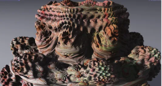
Figure 6: Mandelbulb fractal displayed with our rendering engine.
Maximum quality was reached after 156.2ms render time. Shadows were at maximum quality after 436.2ms. GPU utilisation was 97-99%. GPU: NVidia 640M (480 GFLOPS).
The rendering engine supports operating in a progressive mode, which means when the camera is not moving, the image quality continues to increase. Therefore, the engine is optimised for static scenes. The C++ and OpenGL implementation is highly efficient achieving near 100% GPU utilisation and provides several features.
Firstly, swapping algorithms between passes was a free operation due to the OpenGL subroutines running on the GPU. This and the algorithms inter-compa-
tibility can be used for a short statistical training to determine the best schedule of algorithms for a given scene.
Secondly, a CSG model creator was also implemented. The user can either write the program computing the SDF directly or build the CSG tree from primitives and other program codes both using a built-in graphical interface.
Finally, the shader programs, including subroutines, were generated on-the- fly, thus the code for the scene geometry is embedded into the code running on the GPU. This greatly reduced both the distance function evaluation times and memory consumption.
7. Summary
This paper presented a direct signed distance function visualisation framework and its application to rendering algebraic surfaces.
We proposed a local signed distance function estimation method to such sur- faces and investigated the precision of various surface normal estimation heuristics.
We benchmarked the performance of the system by rendering complex scenes in- corporating CSG elements, meta-surfaces, and the Mandelbulb fractal.
The framework proved to be highly efficient. In addition, it is highly modular, and outperformed current fractal-viewers [3, 4, 7, 9] in both quality and speed.
References
[1] Kenneth Eriksson, Donald Estep, and Claes Johnson. Applied Mathemat- ics: Body and Soul. Number 978-3-540-00890-3. Springer-Verlag Berlin Heidelberg, 1 edition, 2004. Volume 1: Derivatives and Geometry in IR3.
[2] Gerald Farin.Curves and Surfaces for Computer Aided Geometric Design (3rd Ed.):
A Practical Guide. Academic Press Professional, Inc., San Diego, CA, USA, 1993.
[3] Paul Geisler, Daniel White, Paul Nylander, Tom Lowe, David Makin, Buddhi, Joy Leys, Knighty, and Jan Kadlec. Online fractal viewer: FractalLab.
http://hirnsohle.de/test/fractalLab/, 2010.
[4] Matthew Haggett. Mandelbulb 3D (MB3D) fractal rendering software. http://
mandelbulb.com/2014/mandelbulb-3d-mb3d-fractal-rendering-software/, 2014.
[5] John C. Hart. Sphere tracing: A geometric method for the antialiased ray tracing of implicit surfaces.The Visual Computer, 12:527–545, 1994.
[6] Benjamin Keinert, Henry Schäfer, Johann Korndörfer, Urs Ganse, and Marc Stamminger. Enhanced Sphere Tracing. In Andrea Giachetti, editor, Smart Tools and Apps for Graphics - Eurographics Italian Chapter Conference. The Euro- graphics Association, 2014.
[7] Krzysztof Marczak. Mandelbuilder - 3D fractal explorer.
http://www.mandelbulber.com/, 2010.
[8] László Szécsi and Dávid Illés. Real-time metaball ray casting with fragment lists.
In Carlos Andújar and Enrico Puppo, editors, Eurographics (Short Papers), pages 93–96. Eurographics Association, 2012.
[9] Íñigo Quílez. Mandelbulb.
http://www.iquilezles.org/www/articles/mandelbulb/mandelbulb.htm, 2009. (Mandelbulb in real time).