Structure and single particle dynamics of the vapour- liquid interface of acetone-CO
2mixtures
Balázs Fábián,
1George Horvai,
2Abdenacer Idrissi
3and Pál Jedlovszky
4*1
Institute of Organic Chemistry and Biochemistry of the Czech Academy of Sciences, Flemingovo nám. 2, CZ-16610 Prague 6, Czech Republic
2
Department of Inorganic and Analytical Chemistry, Budapest University of Technology and Economics, Szt. Gellért tér 4, H-1111 Budapest, Hungary
3
Laboratoire de Spectrochimie Infrarouge et Raman (UMR CNRS 8516), University of Lille Nord de France, 59655 Villeneuve d’Ascq Cedex, France
4
Department of Chemistry, Eszterházy Károly University, Leányka utca 6, H- 3300 Eger, Hungary
*Electronic mail: jedlovszky.pal@uni-eszterhazy.hu (PJ)
Abstract
Molecular dynamics computer simulations of the liquid-vapour interface of acetone- CO2 mixtures are performed in the canonical (N,V,T) ensemble at 30 thermodynamic state points, ranging from 280 to 460 K and from about 10 to 116 bar, covering the entire composition range from neat CO2 to neat acetone. The molecules forming the first layer at the molecularly rough liquid surface as well as those of the next three subsurface molecular layers have been identified by the ITIM method, and the surface properties of the liquid phase are analyzed in a layer-wise manner. The arrangement of the molecules both within the macroscopic plane of the interface and along its normal axis, as well as their surface orientation and single particle dynamics at the liquid surface are analyzed in detail. It is found that, in accordance with their higher affinity to the vapour phase, CO2 molecules are enriched at the liquid surface, moreover, even within the surface layer they prefer to occupy positions that are more exposed to the bulk vapour phase than those preferred by acetone. In other words, within the molecularly wavy surface layer, CO2 molecules prefer to stay at the crests, while acetone molecules prefer to stay in the troughs. On the other hand, the lateral arrangement of the surface molecules is found to be more or less random. Both molecules prefer to stay perpendicular to the liquid surface, but this preference only involves the first molecular layer, and this preference is governed by the electrostatic interaction of the surface molecules. Both molecules perform considerable lateral diffusion at the liquid surface during their stay there, this diffusion being faster for the CO2 than for the acetone molecules, but not as much faster than in the bulk liquid phase.
Keywords: acetone-CO2 mixtures; liquid-vapour interface; computer simulation; intrinsic surface analysis
1. Introduction
The use of supercritical fluids in a number of industrial processes has become a rapidly growing field of chemistry in the past decades. Besides their initial application in the environmentally friendly destruction of hazardous wastes [!1-4], supercritical fluids are now also widely used as replacements of volatile organic solvents in various separation and reaction processes in, e.g., nanotechnology or polymer technology [!5-9].
Among the possible supercritical solvents, the far most widely used one is CO2 due to its natural abundance, non-toxicity, chemical inertness including non-flammability, relatively low critical temperature (i.e., 304.2 K) [!10] and low cost. Although the physico-chemical properties of supercritical CO2 can be fine tuned through the temperature and pressure, the main limitation of the use of this system is its poor ability of solvating polar solutes. This solvation ability can be dramatically enhanced by adding suitably chosen co-solvents to the system, in particular, weak bases, such as acetone, that can complement the weakly acidic character of CO2. The physico-chemical as well as solvation properties of such mixtures, often referred to as CO2-expanded liquids [!11], can then be fine tuned also through changing their composition. For this reason, both the properties, including also the solvation properties [!12,13] of one phase acetone-CO2 mixtures [!12-22], and the vapour-liquid equilibrium of such mixtures below the critical point [!10,23-38] have been intensively studied in the past decades both by experimental and computer simulation methods.
Besides having accurate information about the thermodynamic behaviour of both the coexisting liquid and vapour phases, and the one phase mixtures of acetone and CO2, the detailed, molecular level characterization of the structure and dynamics of the vapour-liquid interface itself of these systems is also of great importance, as this interface also plays a vital role in a number of processes, such as extraction or catalysis. However, in spite of the aforementioned wealth of studies concerning the thermodynamics of the acetone-CO2
mixtures, including vapour-liquid coexistence, and the existence of detailed computer simulation analyses of the interface between supercritical CO2 and aqueous systems [!39-41], we are not aware of any study targeting the properties of the liquid-vapour interface itself in CO2-expanded liquids.
In describing molecular level properties of disordered phases, computer simulation methods play an important role, as they can provide such a deep insight into the suitably chosen model of the system of interest that cannot be reached by any experimental method,
given that the model used is successfully validated against existing experimental data [!42].
However, analyzing a liquid-vapour interface in computer simulation, i.e., when the interfacial region is seen at atomistic resolution, is not a trivial task, at all. The difficulties in this respect stem from the fact that the liquid surface is corrugated, on the molecular length scale, by capillary waves [!43], and hence both the real, molecularly rough “intrinsic”
covering surface of the liquid phase, and also the list of the interfacial molecules (i.e., the ones that are located at the boundary of the two phases) are difficult to be obtained. The problem is further exacerbated by the fact that the intrinsic surface inherently depends also on a free parameter, representing the length scale on which the interface is seen [!44]. It was repeatedly shown that the simple way of associating the interface with the region of intermediate densities between the two phases along the macroscopic interface normal axis leads to a systematic error of unknown magnitude in the calculated interfacial properties [!45,46], and this systematic error can even propagate to the calculated thermodynamic properties of the system [!47].
Interestingly, this problem was already pointed out in the very first simulations of fluid interfaces by Linse [!48] and Benjamin [!49], who divided the simulation box into several slabs parallel with the macroscopic interface normal, and detected the position of the interface in each slab separately. The first method that can accurately detect the intrinsic surface was proposed by Chacón and Tarazona [!50-52], followed by the development of several alternative methods [!44,45,53-56], some of which are even free from the assumption that the interface is macroscopically flat [!55-56]. Among these methods, the Identification of the Truly Interfacial Molecules (ITIM) [!45] turned out to be an excellent compromise between computational cost and accuracy [!44]. In an ITIM analysis, the liquid surface is probed by a test sphere, moved along grid lines parallel with the macroscopic surface normal from the bulk opposite phase towards the surface to be analyzed. Once the probe touches the first molecule of the phase of interest, this molecule is identified as being part of the interfacial layer, and the probe is moved along the next grid line. Once all grid lines have been considered, the full list of the truly interfacial molecules (i.e., the ones that are “seen” by the probe from the opposite phase) are obtained. Disregarding the interfacial molecules, and repeating the entire algorithm again allows also the identification of the molecules forming the subsequent molecular layers beneath the liquid surface [!45]. In the past decade, intrinsic surface analyzing methods have successfully been applied to study the properties of the surface of various neat molecular liquids [!44-46,53,54,57-61] and binary liquid mixtures [!62-68], ionic liquids [!69-73], mixtures of ionic and molecular liquids [!74], aqueous
electrolyte [!75-77] and surfactant [!78-81] solutions as well as lipid membranes [!82]. In these studies, among others, adsorption [!62-68] and lateral self-aggregation of like molecules [!65,83] at the surface of multicomponent liquid mixtures, orientational preferences, including their dependence on the local curvature of the surface [!44-46,54,57-74], as well as the dynamics [!77,84-87] of the surface molecules have been investigated in detail. Important problems, such as the explanation of the surface tension anomaly of water [!88,89], the feasibility of the ‘HCN World’ hypothesis concerning the prebiotic formation of biomolecules [!65], competitive adsorption of polymers and surfactants [!79,80], the immersion depth of various surfactants in water [!81] as well as the contributions of the subsequent molecular layers [!90] and of the different molecules and moieties [!91,92] to the surface tension have been successfully addressed. Further, the intrinsic profiles of several physical quantities, such as the density [!50-52,54,58,93,94], energy [!94], solvation free energy [!95,96], lateral pressure [!90,94], and electrostatic potential [!75] have been calculated.
In our previous paper [!38], we presented a detailed analysis of the vapour-liquid equilibrium and surface tension of acetone-CO2 mixtures of various compositions below but at the vicinity of their respective critical points on the basis of extensive computer simulations. We also determined, for the first time, the critical point of these mixtures in the entire composition range in two independent ways [!38]. However, we have not analyzed yet the properties of the liquid-vapour interface of these systems. In this paper, we present a detailed analysis of the molecular level structure of the intrinsic liquid surface, as detected by the ITIM method, on the basis of our earlier simulations [!38] covering the entire composition range between the two neat liquids and the range of temperatures between 280 K and 460 K.
The analyses are extended to the second and third subsurface molecular layers of the liquid phase. The composition, width and separation of these layers, the surface adsorption, lateral self-aggregation, surface orientation and surface dynamics of both types of molecules, as well as the composition and temperature dependence of these properties are discussed in detail.
The paper is organized as follows. In sec. 2, details of the calculations performed are given. The obtained results are discussed in detail in sec. 3. Finally, in sec. 4 the main conclusions of this study are summarized.
2. Computational details
2.1. Molecular dynamics simulations
Molecular dynamics simulations of the liquid-vapour interface of acetone-CO2
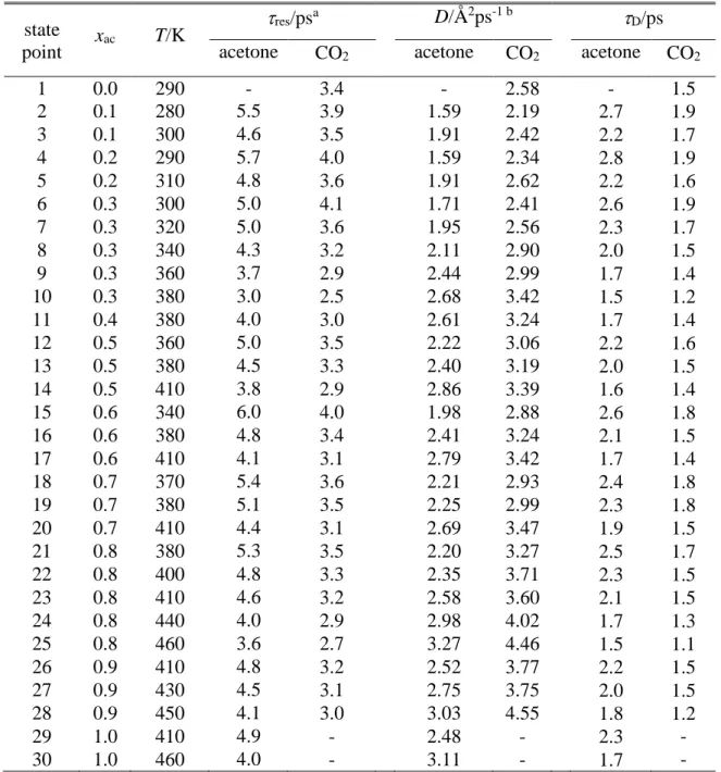
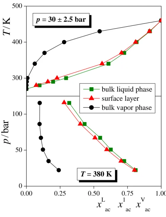
mixtures of 11 different compositions, ranging from neat acetone to neat CO2 with acetone mole fraction increments of 0.1, have been performed in the canonical (N,V,T) ensemble at 30 different thermodynamic state points. The temperature of the systems falls in the range between 280 and 460 K, while their pressure has turned out to be between 10 and 116 bar [!38]. The thermodynamic state points considered, illustrated in Figure 1, have been chosen in such a way that several isotherms (i.e., 380 K and 410 K), isobars (i.e., 30 ± 2.5 bar and 50 ± 2.5 bar) and compositions (i.e., the overall acetone mole fractions of 0.3 and 0.8, being always close to the bulk liquid phase value) [!38] consists of at least 5 state points. The temperature (T), pressure (p) and overall acetone mole fraction (xac) of the systems simulated are summarized in Table 1. Details of the simulations have been described in our previous publication [!38], thus, they are just reminded here. The rectangular basic simulation box has contained 4000 molecules, while the length of its Y and Z edges, both being parallel with the macroscopic plane of the interface, has been 50 Å in every case. The LX length of the edge X as well as the number of acetone and CO2 molecules (Nac and NCO2, respectively), the simulation temperature and the pressure of the systems considered in this analysis are collected in Table 1.
Both the acetone [!97] and CO2 molecules [!98] have been described by the Transferable Potential for Phase Equilibria (TraPPE) force field. These models are not only able to accurately reproduce a number of properties of the two neat systems [!97,98], but their combination turned out to be superior over other ones in describing the thermodynamics of mixing of the two compounds [!22], and was recently shown to excellently reproduce the vapour-liquid coexistence of these mixtures in the entire composition range in which such experimental data exist [!38]. Since the TraPPE potential model family is pairwise additive [!97-99], the total potential energy of the system, apart from the long range correction terms, is calculated as the sum of the contributions of all molecule pairs, and the interaction energy of a molecule pair is given as the sum of the Coulomb and Lennard-Jones contributions of all pairs of their interaction sites:
j i
n n
j i j
i
ij r
q q r
u r
i j
, 1 1 0
6
, 12
, 4
4 1
. (1)
In this equation, indices i and j refer to the two interacting molecules, indices and run over all the ni and nj interaction sites of molecules i and j, respectively, and are the Lennard-Jones energy and distance parameters, respectively, of the interaction site pair and
, q and q are the fractional charges carried by the respective interaction sites, ri,j is the distance of site on molecule i from site on molecule j, and 0 is the vacuum permittivity.
The Lennard-Jones parameters characteristic to the interaction site pairs and are related to the ones corresponding to the individual sites through the Lorentz-Berthelot combination rule [!42]. Both potential models are rigid; the interaction sites of the CO2 molecule coincide with the atomic positions [!98], while the CH3 groups of the acetone molecule are treated as united atoms [!97]. The interaction parameters corresponding to the individual interaction sites of the two molecules are summarized in Table 2. According to the original parameterization of the TraPPE force field [!97-99], long range correction has been applied both for the electrostatic and dispersion term.
The simulations have been done using the GROMACS 5.1 package [!100]. All parameters of the simulations have been set according to a recent benchmark study of the united atom TraPPE force field [!101]. Thus, equations of motion have been integrated in time steps of 2 fs, the geometry of the molecules has been set by the LINCS algorithm [!102], the temperature of the systems has been kept constant using the Nosé-Hoover thermostat [!103,104] with the coupling parameter of 0.5 ps, and the long range correction of both the electrostatic and dispersion interactions has been calculated by the smooth variant of the Particle Mesh Ewald method [!105,106], using a centre-centre cut-off distance of 12 Å, a reciprocal space grid of 1.5 Å-1, and a spline order of 4. In the simulations, the system has always been equilibrated for at least 20 ns. Then, in the 10 ns long production stage, 5000 sample configurations, separated from each other by 2.0 ps long trajectories, have been dumped for detailed analyses. In all the analyses, averaging has not only been performed over all the sample configurations, but also over the two vapour-liquid interfaces present in the basic box.
2.2. ITIM Analysis
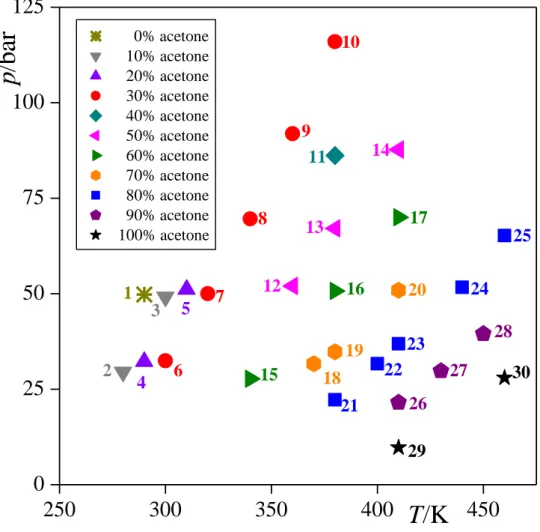
The molecules pertaining to the intrinsic liquid surface as well as to the two subsequent molecular layers have been identified by means of the ITIM method [!45], using the freely available [!107] PYTIM software package [!108]. Test lines parallel with the edge X of the basic box have been arranged in a square grid with a grid space of 0.5 Å. According to previous studies concerning the optimal size of the probe sphere [!44,45,109], its radius has been set to 2 Å. In determining the contact position of the probe with a molecule, all the atoms (and united atoms) have been treated as spheres the diameter of which is equal to the corresponding Lennard-Jones distance parameter, . Upon approaching the critical point, when the density of the two phases becomes increasingly similar to each other, the separation of liquid and vapour phases becomes a non-trivial task. We have distinguished between the molecules pertaining to the liquid and vapour phases by means of the DBSCAN algorithm [!110], implemented also in the PYTIM package, using the cluster cut-off value of 10 Å and an automatic density threshold determination scheme [!74]. Equilibrium snapshots of the interfacial portion of the systems consisting of acetone in the overall mole fractions of 0.3, 0.5 and 0.8, indicating also the first four separate molecular layers beneath the liquid surface, are shown in Figure 2 as obtained from the simulations at 380 K.
3. Results and discussion
3.1. Density profiles
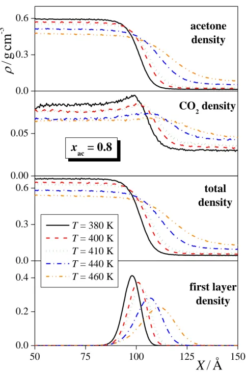
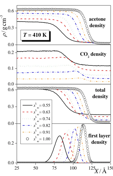
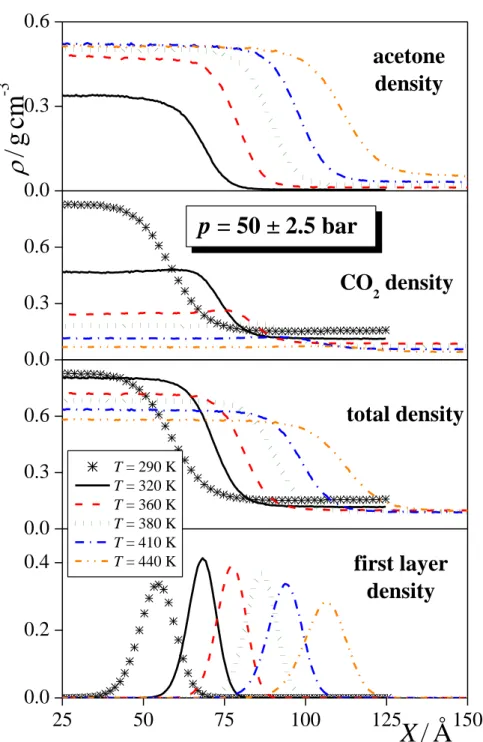
The total mass density profile as well as the contributions of the acetone and CO2
molecules to this profile are shown in Figure 3, as obtained in several systems corresponding to the overall acetone mole fraction of 0.8 (being very close to the bulk liquid phase acetone mole fraction, as well), to the temperature of 410 K, and to the pressure of 50 ± 2.5 bar. As is seen, the total mass density profiles as well as the acetone contributions change smoothly between the bulk liquid and vapour phases, while the CO2 profiles exhibit a small peak at the liquid side of the interface, indicating the enrichment of the CO2 molecules at the interfacial region. This adsorption of the CO2 molecules at the liquid-vapour interface is, in general, stronger at lower temperatures and pressures, and at higher acetone mole fractions. However, the density corresponding to the interfacial peak of the CO2 profile never exceeds the bulk liquid phase value by more than 15%, indicating that this adsorption is rather weak. This is
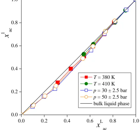
illustrated in Figure 4, showing the acetone mole fraction in the surface layer, x1ac, as a function of the bulk liquid phase acetone mole fraction, xacL , as obtained at the 380 K and 410 K isotherms as well as at the 30 ± 2.5 bar and 50 ± 2.5 bar isobars. As is seen, the surface layer of the liquid phase contains acetone molecules in a lower mole fraction than the bulk liquid phase, but this difference is rather small, being in the order of 10-20%, certainly much smaller than the similar difference between the bulk liquid and vapour phase acetone mole fractions (the latter being denoted byxacV) [!38]. This is illustrated in Figure 5, showing the coexisting liquid and vapour phase acetone mole fractions along with that in the surface layer at the pressure of 30 ± 2.5 bar and at the temperature of 380 K. The acetone mole fractions corresponding to the bulk liquid and vapour phases as well as to the first four subsurface layers of the systems simulated are collected in Table S1 of the supplementary material.
The contribution of the molecules constituting the surface layer to the overall density profile is also shown in Figure 3 (bottom panels). As is seen, this contribution always extends deeply into the X range where the corresponding total mass density profile reaches its bulk liquid phase value. Conversely, the second and, in many cases, also the third subsurface layer gives contribution to the intermediate density region of the total profile (as illustrated in Figure S1 of the supplementary material for selected state points). These findings stress again the importance of identifying the real, capillary wave corrugated intrinsic liquid surface in the analyses. Clearly, defining the interfacial region through the intermediate density part of the total density profile would cause a large systematic error in the calculated properties due to the misidentification of a large number of molecules as being (or not being) at the liquid surface.
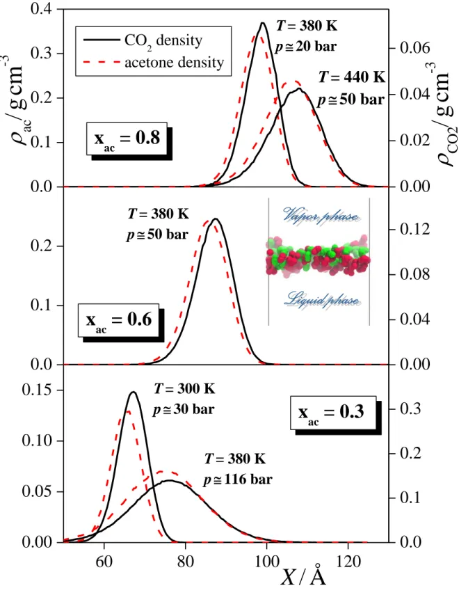
Besides the density profile of the entire surface layer, we have also calculated the contributions of the acetone and CO2 molecules to this profile. These contributions are compared in Figure 6 in five thermodynamic state points. As is seen, the profile corresponding to the surface CO2 molecules is always shifted noticeably, by about 2 Å towards the vapour phase with respect to the corresponding acetone profile, and this shift does not depend on the temperature, pressure and composition of the system. Considering that the magnitude of this shift of about 2 Å is comparable with the distance of the two O atoms of the CO2 molecule or with that of any two non-neighbouring interaction sites of the acetone molecule, we conclude that this shift cannot be explained simply by the orientation of the surface molecules. Instead, it indicates a real preference of the CO2 molecules to be located
closer to the bulk vapour phase within the surface layer than the acetone molecules. Such positions are available at the crests of the molecularly rugged surface layer, where the molecules are more exposed to the vapour phase. Conversely, interfacial acetone molecules prefer to stay at the troughs of the molecularly rough surface layer, where they are better surrounded by their liquid phase neighbours. The observed preference of the interfacial CO2
molecules for being strongly exposed to the vapour phase, illustrated in the inset of Fig. 6 on the example of the equimolar system at 360 K, is consistent with their above discussed surface adsorption as well as with their marked enrichment in the vapour phase [!38].
The density profiles of the surface layer as well as of the subsequent subsurface layers can always be very well fitted by a Gaussian function [!111]. The position and width parameters of this Gaussian function, denoted here as X0 and , respectively, can serve as estimates of the average position and width of the corresponding molecular layer. Further, the difference of the X 0 values of two subsequent layers, X0, characterizes the spacing between these layers. The and X0 values corresponding to the first four layers of all systems simulated are collected in Table S2 of the supplementary material.
As is seen, the average distance of the first and second layers (X0) is typically about 10% larger than that of the second and third as well as of the third and fourth ones, and this picture is independent from the composition and thermodynamic state of the system. This finding is related to the fact that the surface layer is much less strongly confined by its neighbours at its vapour than its liquid side. On the other hand, the width of the subsequent layers () is rather similar to each other. Although a slight shrinking of the subsurface layers upon going from the surface towards the bulk liquid phase can be observed in some of the systems, this shrinking never exceeds 5% from the first to the fourth layer, and in the neat systems and systems of large acetone mole fractions it is negligible.
The width of the first layer shows, however, a strong dependence on the composition and thermodynamic state of the systems. Thus, its value increases, in general, with increasing temperature (and, correspondingly, also with increasing pressure) and with decreasing acetone mole fraction. The dependence of the inverse width of the first layer, -1, on the temperature at constant pressure (top) and at constant liquid composition (bottom), as well as on the pressure at constant temperature (top) and at constant liquid composition (bottom) are shown in Figure 7.a and 7.b, respectively. As is seen, while -1 decreases monotonously with increasing pressure at constant temperature (top of Fig. 7.b), its temperature dependence exhibits a clear maximum along both isobars considered (top of Fig. 7.a). The origin of this maximum
behaviour is not clear. On one hand, it is probably related to the fact that the critical pressure of this mixture goes through a maximum around the liquid phase acetone mole fraction of 0.3 [!38], and hence, along an isotherm, the state points of this composition are the farthest from the critical point, and thus correspond to the narrowest surface layer. On the other hand, however, the width of the surface layer might also well depend on the composition of the surface layer even if the different state points are at the same relative distance from the critical temperature.
At constant liquid phase composition, the reciprocal width seems to decrease linearly both with the temperature and with the pressure. In principle, the T or p value at which the reciprocal width reaches zero (and, hence, the width of the surface layer becomes infinite) could serve as an estimate of the critical temperature or pressure corresponding to this composition [!47]. However, the temperature values obtained this way exceed the critical temperature of the system, determined earlier in two independent ways (i.e., from the temperature dependence of both the coexisting liquid and vapour phase densities and of the surface tension) [!38] by 40-80 K. Similarly, the pressure value at which -1 becomes zero is always 15-40 bar higher than the critical pressure as obtained through the Clausius-Clapeyron equation [!38]. The comparison of the critical temperature and pressure values as obtained in different ways is shown in Figure S2 of the supplementary material, together with available experimental data. In understanding the reason of the apparent failure of this extrapolation in reliably estimating the critical parameters, one has to consider that the pressure in vapour- liquid equilibrium depends exponentially on the temperature (according to the Clausius- Clapeyron equation), and hence no quantity, including evidently also -1, can be a linear function of both T and p at the same time. Thus, the apparent linear decay of the -1(T) and
-1(p) data points is probably only true at states far enough the critical point (such as those corresponding to our simulations), and, upon approaching the critical point, they are expected to progressively deviate from the linear behaviour, making the estimates based on the linear extrapolation unreliable.
3.2. Lateral arrangement of the surface molecules
Besides analyzing their distribution along the interface normal axis, we have also investigated the lateral arrangement of the surface molecules within the macroscopic plane of the interface, YZ. In particular, we focus on the possible lateral self-aggregation of the like molecules at the liquid surface. This problem can be investigated by calculating the area
distribution of the Voronoi cells [!112] of the molecules in the macroscopic plane of the interface. Namely, if the particles are uniformly distributed in the YZ plane, the distribution of the area (A) of their Voronoi cells follows a gamma distribution [!113], i.e.,
P(A)aA1exp
A
, (2) where the parameter a normalizes the distribution to unity, while and are adjustable parameters. On the other hand, if the particles show noticeable lateral aggregation, the P(A) distribution exhibits a tail of exponential decay at the large A side of its peak [!114]. Thus, lateral self-aggregation of a certain type of particles (i.e., either acetone or CO2) can be studied by disregarding the other component, and calculate the P(A) distribution considering only the molecules of interest [!115]. To perform this analysis, we have projected the central atom (i.e., the C atom of the C=O group for acetone and the C atom of CO2) of the molecules of interest, belonging to the surface layer, to the YZ plane, and calculated the P(A) distribution of these projections. The resulting distributions, together with their best fitting gamma functions (eq. 2) are shown in Figure 8 as obtained for the surface acetone and CO2 molecules at constant composition, temperature, and pressure.As is seen, the calculated P(A) distributions can always be very well fitted by the gamma function, indicating that neither of the two components exhibit considerable lateral self-association. In other words, our results reveal that the acetone and CO2 molecules of the surface layer are distributed more or less randomly within the macroscopic plane of the surface. This is illustrated in Figure 9, showing the projected centres of the surface molecules in a sample equilibrium configuration as obtained at 380 K in systems of three different compositions.
3.3. Orientational preferences of the surface molecules
The orientation of a rigid molecule of general shape relative to an external plane or direction can fully be described by two independent orientational variables. As a consequence, the analysis of the orientational statistics of such molecules relative to the macroscopic plane of the liquid surface (or to its normal) requires the calculation of the joint bivariate probability distribution of such an independent orientational parameter pair [!116,117]. As we demonstrated it previously, the choice of the two angular polar coordinates,
and , of the interface normal vector in a local Cartesian frame fixed to the individual molecules is a sufficient choice of such a parameter pair [!116,117]. This picture simplifies in
the case of linear molecules, the surface orientation of which can fully be described by one single orientational variable. For the acetone molecules, here we define the aforementioned local frame in the following way. Its origin is fixed to the central C atom, axis x is the molecule normal, axis z points along the C=O bond in such a way that the z coordinate of the O atom is negative, while axis y is parallel with the line joining the two CH3 groups. For the linear CO2 molecule, the single orientational parameter we use here is the angle formed by the molecular axis and the surface normal. By our convention, the surface normal vector, X, is oriented in such a way that it points from the liquid to the vapour phase. The definition of the above local Cartesian frame as well as of the orientational variables , and are illustrated in Figure 10.a. It should be emphasized that the angles and are formed by two general spatial vectors, but the two vectors forming the angle are restricted to lay in a given plane (i.e., the xy plane of the local frame) by definition. Therefore, uncorrelated orientation of the molecules with the surface normal results in uniform distribution only if cos and , or cos
are used as orientational variables [!116,117]. Further, due to the symmetry of the molecules, these orientational variables can always be chosen in such a way that the relations 0o ≤ ≤ 90o and 0 ≤ cos ≤ 1 hold.
To study also whether the molecules adopt different orientations at portions of different curvature of the molecularly wavy liquid surface, we have divided the surface layer to three separate regions according to its density profile. These regions are defined as follows.
Region A extends from the vapour phase to the X value at which the density of the surface layer reaches half of its maximum value; region B covers the X range in which the surface layer density exceeds half of its maximum value, while region C is located between the X value where the surface layer density drops again to half of its maximum value and the bulk liquid phase. Thus, regions A and C cover typically the positively curved crests and negatively curved troughs of the wavy liquid surface. The definition of regions A, B and C of the surface layer is illustrated in Figure 10.b. It should be noted that, in accordance with our previous conclusion, we have also found 40-80% more acetone molecules in region C (i. e. at the troughs of the surface) than in region A, and conversely, the number of CO2 molecules located in region A has been found to exceed that in region C by 20-100% in every case.
The P(cos,) orientational maps of the acetone molecules in the entire surface layer as well as in its separate regions A, B and C are shown in Figure 11 as obtained in five different state points. The distributions exhibit increasing probabilities with increasing cos
values, and their maximum is always located around the {cos = 1; = 90o} point. It should
be noted that in the case of cos = 1 the surface normal axis points along the z axis of the local frame, and hence the polar angle loses its meaning (see Fig. 10.a). As a consequence, all points of the P(cos,) map laying along the cos = 1 line are equivalent, they all correspond to the same orientation, i.e., when the plane of the acetone molecule is perpendicular to the macroscopic plane of the liquid surface, YZ, and the C=O bond points straight to the liquid phase. The preference for this orientation can be understood considering that this way the apolar methyl groups are exposed to the vapour phase, while the strongly dipolar C=O group is immersed to the liquid phase. The fact that the maximum of the bivariate distribution occurs around the = 90o point of this line reveals that deviations from this preferred orientation occur more frequently by the rotation of the molecule around its normal axis, x (i.e., when the molecule remains still perpendicular to the YZ plane) than around any other axis (i.e., when this rotation also tilts the entire molecule from its perpendicular alignment). The preferred orientation of the surface acetone molecules relative to the surface normal vector, X, together with the rotation corresponding to the preferred deviation from this alignment is illustrated at the bottom of Fig. 11. It should be noted that similar orientational preferences are seen in all the three separate regions of the surface layer, these preferences being the strongest in region C and the weakest in region A. Further, the orientational preferences are found to be insensitive to the composition of the system, while the increase of the temperature leaves the orientational preferences themselves unchanged but makes them considerably weaker.
The distribution of cos, describing the surface orientation of the CO2 molecules, is shown in Figure 12 as obtained in the surface layer in state points corresponding to the overall acetone mole fraction of 0.3 and to the temperature of 380 K. Very similar distributions have been obtained in regions A, B, and C of the surface layer (not shown). As is seen, the maximum of the distribution always occurs at cos = 1, indicating that the CO2 molecules prefer to stay perpendicular to the macroscopic plane of the liquid surface. The preference of the CO2 molecules for this alignment, illustrated also at the bottom of Fig. 11, clearly increases with increasing acetone mole fraction (see the bottom panel of Fig. 12). This finding suggests that the physical reason behind this orientational preference is the interaction of the strongly quadrupolar CO2 molecules with the large dipole moment located along the C=O bond of the acetone molecules, which also stays preferentially perpendicular to the liquid surface. Further, the orientational preference of the CO2 molecules, similarly to that of acetone, is found to be stronger at lower temperatures. Finally, it should be noted that no
considerable orientational preference of any of the two molecules have been found already in the second layer beneath the liquid surface in any of the state points considered.
3.4. Dynamics of the surface molecules
In investigating the dynamics of the surface molecules, we have calculated their survival probability and mean residence time within the surface layer as well as in the subsequent three layers, and also their lateral diffusion coefficient within the surface layer.
3.4.1. Survival probability and mean residence time in the subsurface layers. The survival probability, L(t), of the particles at the liquid surface is the probability that a particle that belongs to the surface layer at t0 stays uninterruptedly in this layer until at least t0+t. Since the departure of a particle from the liquid surface is a process of first order kinetics, the L(t) probability is expected to follow exponential decay. Further, if a particle can leave the surface layer by several different mechanisms (e.g., temporarily by a vibration or permanently by diffusion), L(t) is the sum of as many exponentials as the number of the possible mechanisms.
Although L(t) usually follows a biexponential decay, here we could always fit it by one single exponential,
) / exp(
)
(t A t res
L , (3)
presumably because the time scales corresponding to the different mechanisms are rather close to each other. In eq. 3, the parameter res denotes the mean residence time of the particles within the surface layer. This parameter sets the time scale of the processes that can be meaningfully analyzed as occurring within the surface layer. Namely, for processes occurring on time scales longer than res, the particles are exchanged between the surface layer and the rest of the system during this process is in course, and hence, from the point of view of this process, surface and non-surface particles cannot be distinguished from each other.
The mean surface residence time values of the acetone and CO2 molecules are collected in Table 3 as obtained in the surface layer, while the values corresponding to the first four subsurface molecular layers are included in Table S3 of the supplementary material.
Further, the acetone and CO2 survival probabilities in the surface layer are shown in Figure 13, as obtained at several state points corresponding to the overall acetone mole fraction of 0.3, and to the temperature of 380 K. To emphasize the single exponential decay of these curves, the survival probabilities are shown on a logarithmic scale, thus, the exponentially decaying L(t) data are transformed to straight lines.
As is seen, the mean surface residence time of the molecules always falls between 3 and 6 ps, being 30-50% larger for the acetone than for the CO2 molecules. Further, it increases with increasing acetone mole fraction and with decreasing temperature for both molecules, as illustrated in the insets of Fig. 13. The res values obtained in the second layer are 30-50%
smaller for acetone and 10-20% smaller for CO2 than those in the surface layer. Further, the values corresponding to the third and fourth layer are always very close to those of the second one, indicating that, from the second layer on, the dynamics of the molecules is essentially bulk-like.
3.4.2. Lateral diffusion at the liquid surface. The lateral diffusion coefficient (i.e. that within the YZ plane) of the surface molecules, D, can be calculated through the Einstein relation [!42], i.e., D = MSD/4t, by fitting a straight line to the calculated MSD vs. t data. Here MSD denotes the mean square lateral displacement of the particles during the time t. To ensure that the particles are no longer in the ballistic regime and indeed perform diffusive motion, the first 2 ps of the MSD(t) data (i.e., the first data point) has been omitted from the fitting procedure. It should be emphasized that, in calculating the lateral diffusion coefficient of the surface molecules, each molecule is taken into account only as long as it stays uninterruptedly within the surface layer. The characteristic time of the surface diffusion, D, is defined as the time required for a molecule to fully explore the surface area per molecule (or, equivalently, the time at which MSD reaches the surface area per molecule). The value of D
can simply be calculated as [!77,85-87,118]
D N
YZ
surf D 2
, (4)
where <Nsurf> is the average number of the molecules in the surface layer.
The values of D and D are collected in Table 3 as obtained for both types of molecules in every system considered. As is seen, the value of D is about half of res in every case, confirming that both molecules perform considerable lateral diffusion during their stay at the liquid surface. Among the two molecules, CO2 diffuses considerably faster, as its lateral diffusion coefficient is 40-50% larger than that of acetone in every system. This finding can largely be attributed simply to the larger mobility of the CO2 than the acetone molecules, which is also apparent in the bulk liquid phase of the systems. Further, the ratio of the CO2
and acetone diffusion coefficients is somewhat, by about 10% larger in the bulk liquid phase
than in the surface layer. In other words, the vicinity of the vapour phase enhances the diffusion of the acetone molecules more than that of the CO2 molecules. The reason of this is probably that the acetone molecules, forming strong dipole pairs with their nearest neighbours in the bulk liquid phase [!119], are less tethered by these strong dipole-dipole interactions at the liquid surface due to the lack of such neighbours at the vapour side. On the other hand, CO2 molecules are not involved in such strong directional interactions with their nearest neighbours, and hence they are somewhat less affected by the lack of their vapour side neighbours at the interface.
The temperature and composition dependence of the lateral diffusion coefficient of the surface molecules is illustrated in Figure 14. As is seen, it increases with increasing temperature for both molecules. The diffusion coefficient of the acetone molecules decreases with increasing acetone mole fraction, presumably due to the increasing dipole-dipole interaction of the neighbouring acetone molecules. On the other hand, the composition dependence of D is less clear for CO2, the present data suggest that it probably goes through a minimum around the equimolar composition. However, further analysis of this behaviour would require additional simulations.
4. Summary and Conclusions
In this paper, a detailed analysis of the interfacial structure and dynamics has been performed at the free liquid surface of acetone-CO2 mixtures of various compositions, ranging from neat CO2 to neat acetone. The thermodynamic states considered cover a rather broad range, extending from 280 to 460 K and from 10 to 116 bar. The real, intrinsic surface of the liquid phase is identified by means of the ITIM method, and the analyses are extended to the first four molecular layers beneath the liquid surface. The obtained results have clearly revealed that while the properties of the surface layer differ in several respects from those of the subsequent ones, and the system exhibits essentially bulk-like behaviour from the second layer on.
In accordance with their higher concentration in the vapour than in the liquid phase [!38], CO2 molecules are present at the liquid surface in a somewhat higher mole fraction than in the bulk liquid phase. This weak adsorption is, however, only extended to the first molecular layer of the liquid phase. Further, within the surface layer, CO2 molecules prefer to be more exposed to the vapour phase than acetones, thus, they are preferentially located at the crests, while acetone molecules in the troughs of the molecularly wavy liquid surface. On the
other hand, the lateral arrangement of the two types of molecules in the surface layer is rather similar to each other; no lateral self-aggregation of either of the two components has been observed.
The average distance of the surface layer from the second one is somewhat, i.e., about 10% larger than the average separation of any two subsequent neighbouring layers, and the first layer is also slightly wider, on average , than the subsequent ones. The width of the first layer increases with increasing temperature and pressure. Although the reciprocal width of the surface layer seems to decays linearly with T and p, extrapolation to its zero value has turned out to be a rather crude and inaccurate way of estimating the critical temperature and pressure, presumably because they expected to deviate from this linear behaviour at the vicinity of the critical point.
Both molecules prefer to stay perpendicular to the macroscopic plane of the liquid surface. In the case of acetone, the preferred orientation is such that the C=O bond points straight inward, to the liquid phase. Moreover, acetone molecules can more easily deviate from this preferred orientation in such a way that they still remain perpendicular to the liquid surface (i.e., by a rotation around their molecular normal axis) than by tilting from this perpendicular alignment. These orientational preferences are governed by the dipolar interaction between the acetone molecules and the dipole-quadrupole interaction between acetone-CO2 pairs. Although the orientational preferences themselves do not change with the thermodynamic conditions, they become weaker with increasing temperature and, in the case of CO2, also with decreasing acetone mole fraction.
Although the mean surface residence time of both molecules is rather short, falling between 3 and 6 ps depending on the thermodynamic conditions, it is still about twice as long as the characteristic time of the lateral diffusion of the surface molecules. This finding means that both molecules stay, on average, long enough at the liquid surface to perform considerable lateral diffusion here. The mean surface residence time of both molecules increases with increasing acetone mole fraction and decreasing temperature, and it is considerably, by 30-50% longer for acetone than fro CO2. On the other hand, CO2 molecules diffuse 40-50% faster than acetones, but the ratio of their diffusion coefficients is about 10%
smaller at the liquid surface than in the bulk liquid phase.
Acknowledgements
The authors acknowledge financial support from the NKFIH Foundation, Hungary (project Nos. 134596 and 120075) and from the Hungarian French Intergovernmental Science and Technology Program (TéT, Balaton) under project Nos. 2019-2.1.11-TÉT-2019-00017 (Hungary) and 44706QK (France). Calculations have been performed at Mésocentre de Calcul, a Regional Computing Centre at Université de Franche-Comté.
References
[1] C. A. Eckert, B. L. Knutson, P. G. Debenedetti, Nature 383 (1996) 313-318.
[2] H. J. Bleyl, J. Abeln, N. Boukis, H. Goldacker, M. Kluth, A. Kruse, G. Petrich, H.
Schmieder G. Wiegand, Separation Sci. Technol. 32 (1997) 459-485.
[3] P. E. Savage, Chem. Rev. 99 (1999) 603-622.
[4] H. Weingärtner, E. U. Franck, Angew. Chem. Int. Ed. 44 (2005) 2672-2692.
[5] J. F. Brennecke, J. E. Chateauneuf, Chem. Rev. 99 (1999) 433-452.
[6] A. Baiker, Chem. Rev. 99 (1999) 453-474.
[7] J. L. Kendall, D. A. Canelas, J. L. Young, J. M. DeSimone, Chem. Rev. 99 (1999) 543-564.
[8] C. F. Kirby, M. A. McHugh, Chem. Rev. 99 (1999) 565-602.
[9] K. P. Johnston, P. Shah, Science 303 (2004) 482-483.
[10] A. Bamberger, G. Maurer, J. Chem. Thermodyn. 32 (2000) 685-700.
[11] P. G. Jessop, B. Subramaniam, Chem. Rev. 107 (2007) 2666-2694.
[12] J. L. Gohres, C. L. Kitchens, J. P. Hallett, A. V. Popov, R. Hernandez, C. L. Liotta, C.
A. Eckert, J. Phys. Chem. B 112 (2008) 4666-4673.
[13] D. L. Gurina, M. L. Antipova, E. G. Odintsova, V. E. Petrenko, J. Supercrit. Fluids 139 (2018) 19-29.
[14] H. Pöhler, E. Kiran, J. Chem. Eng. Data 42 (1997) 379-383.
[15] J. Chen, W. Wu, B. Han, L. Gao, T. Mu, Z. Liu, T. Jiang, J. Du, J. Chem. Eng. Data 48 (2003) 1544-1548.
[16] J. Wu, Q. Pan, G. L. Rempel, J. Chem. Eng. Data 49 (2004) 976-979.
[17] M. I. Cabaço, Y. Danten, T. Tassaing, S. Longelin, M. Besnard, Chem. Phys. Letters 413 (2005) 258-262.
[18] C. L. Shukla, J. P. Hallett, A. V. Popov, R. Hernandez, C. L. Liotta, C. A. Eckert, J.
Phys. Chem. B 110 (2006) 24101-24111.
[19] K. Liu, E. Kiran, Ind. Eng. Chem. Res. 46 (2007) 5453-5462.
[20] F. Zahran, C. Pando, J. A. R. Renuncio, A. Cabañas, J. Chem. Eng. Data 55 (2010) 3649-3654.
[21] T. Aida, T. Aizawa, M. Kanakubo, H. Nanjo, J. Supercrit. Fluids 55 (2010) 71-76.
[22] A. Idrissi, I. Vyalov, M. Kiselev, P. Jedlovszky, Phys. Chem. Chem. Phys. 13 (2011) 16272-16281.
[23] T. Katayama, K. Ohgaki, G. Maekawa, M. Goto, T. Nagano, J. Chem. Eng. Jpn. 8 (1975) 89-92.
[24] P. Traub, K. Stephan, Chem. Eng. Sci. 45 (1990) 751-758.
[25] C. Y. Day, C. J. Chang, C. Y. Chen, J. Chem. Eng. Data 41 (1996) 839-843.
[26] C. J. Chang, C. Y. Day, C. M. Ko, K. L. Chiu, Fluid Phase Equilib. 131 (1997) 243- 258.
[27] T. Adrian, G. Maurer, J. Chem. Eng. Data 42 (1997) 668-672.
[28] C. J. Chang, K. L. Chiu, C. Y. Day, J. Supercrit. Fluids 12 (1998) 223-237.
[29] S. D. Moon, B. K. Moon, Bull. Korean Chem. Soc. 21 (2000) 1133-1137.
[30] M. Stievano, N. Elvassore, J. Supercrit. Fluids 33 (2005) 7-14.
[31] F. Han, Y. Xue, Y. Tian, X. Zhao, L. Chen, J. Chem. Eng. Data 50 (2005) 36-39.
[32] W. Wu, J. Ke, M. Poliakoff, J. Chem. Eng. Data 51 (2006) 1398-1403.
[33] Y. Houndonougbo, H. Jin, B. Rajagopalan, K. Wong, K. Kuczera, B. Subramaniam, B. Laird, J. Phys. Chem. B 110 (2006) 13195-13202.
[34] Y. Houndonougbo, K. Kuczera, B. Subramaniam, B. Laird, Mol. Simul. 33 (2007) 861-869.
[35] H. Y. Chiu, M. J. Lee, H. M. Lin, J. Chem. Eng. Data 53 (2008) 2393-2402.
[36] A. A. Novitsky, E. Pérez, W. Wu, J. Ke, M. Poliakoff, J. Chem. Eng. Data 54 (2009) 1580-1584.
[37] C. M. Hsieh, J. Vrabec, J. Supercrit. Fluids 100 (2015) 160-166.
[38] B. Fábián, G. Horvai, A. Idrissi, P. Jedlovszky, J. CO2 Utiliz. 34 (2019) 465-471.
[39] S. R. P. da Rocha, K. P. Johnston, R. E. Westacott, P. J. Rossky, J. Phys. Chem. B 105 (2001) 12092-12104.
[40] N. Galand, G. Wipff, Supramol. Chem. 17 (2005) 453-464.
[41] X. Li, D. A. Ross, J. P. M. Trusler, G. C. Maitland, E. S. Boek, J. Phys. Chem. B 117 (2013) 5647-5652.
[42] M. P. Allen, D. J. Tildesley, Computer Simulation of Liquids, Clarendon Press, Oxford, 1987.
[43] J. S. Rowlinson, B. Widom, Molecular Theory of Capillarity, Dover Publications, Mineola, 2002.
[44] M. Jorge, P. Jedlovszky, M. N. D. S. Cordeiro, J. Phys. Chem. C. 114 (2010) 11169- 11179.
[45] L. B. Pártay, Gy. Hantal, P. Jedlovszky, Á. Vincze, G. Horvai, J. Comp. Chem. 29 (2008) 945-956.
[46] Gy. Hantal, M. Darvas, L. B. Pártay, G. Horvai, P. Jedlovszky, J. Phys.: Condens.
Matter 22 (2010) 284112-1-14.
[47] L. B. Pártay, G. Horvai, P. Jedlovszky, J. Phys. Chem. C. 114 (2010) 21681-21693.
[48] P. Linse, J. Chem. Phys. 86 (1987) 4177-4187.
[49] I. Benjamin, J. Chem. Phys. 97 (1992) 1432-1445.
[50] E. Chacón, P. Tarazona, Phys. Rev. Letters 91 (2003) 166103-1-4.
[51] E. Chacón, P. Tarazona, J. Phys.: Condens. Matter 17 (2005) S3493-S3498.
[52] P. Tarazona, E. Chacón, Phys. Rev. B 70 (2004) 235407-1-13.
[53] J. Chowdhary, B. M. Ladanyi, J. Phys. Chem. B. 110 (2006) 15442-15453.
[54] M. Jorge, M. N. D. S. Cordeiro, J. Phys. Chem. C. 111 (2007) 17612-17626.
[55] A. P. Wilard, Chandler, J. Phys. Chem. B. 114 (2010) 1954-1958.
[56] M. Sega, S. Kantorovich, P. Jedlovszky, M. Jorge, J. Chem. Phys. 138 (2013) 044110- 1-10.
[57] L. B. Pártay, G. Horvai, P. Jedlovszky, Phys. Chem. Chem. Phys. 10 (2008) 4754- 4764.
[58] M. Jorge, M. N. D. S. Cordeiro, J. Phys. Chem. B 112 (2008) 2415-2429.
[59] Gy. Hantal, P. Terleczky, G. Horvai, L. Nyulászi, P. Jedlovszky, J. Phys. Chem. C.
113 (2009) 19263-19276.
[60] M. Darvas, K. Pojják, G. Horvai, P. Jedlovszky, J. Chem. Phys. 132 (2010) 134701-1- 10.
[61] P. Jedlovszky, B. Jójárt, G. Horvai, Mol. Phys. 113 (2015) 985-996.
[62] L. B. Pártay, P. Jedlovszky, Á. Vincze, G. Horvai, J. Phys. Chem. B. 112 (2008) 5428- 5438.
[63] L. B. Pártay, P. Jedlovszky, G. Horvai, J. Phys. Chem. C. 113 (2009) 18173-18183.
[64] K. Pojják, M. Darvas, G. Horvai, P. Jedlovszky, J. Phys. Chem. C. 114 (2010) 12207- 12220.
[65] B. Fábián, M. Szőri, P. Jedlovszky, J. Phys. Chem. C 118 (2014) 21469-21482.
[66] A. Idrissi, Gy. Hantal, P. Jedlovszky, Phys. Chem. Chem. Phys. 17 (2015) 8913-8926.
[67] B. Fábián, B. Jójárt, G. Horvai, P. Jedlovszky, J. Phys. Chem. C. 119 (2015) 12473- 12487.
[68] B. Kiss, B. Fábián, A. Idrissi, M. Szőri, P. Jedlovszky, J. Phys. Chem. C. 122 (2018) 19639-19651.
[69] Gy. Hantal, M. N. D. S. Cordeiro, M. Jorge, Phys. Chem. Chem. Phys. 13 (2011) 21230-21232.
[70] M. Lísal, Z. Posel, P. Izák, Phys. Chem. Chem. Phys. 14 (2012) 5164-5177.
[71] Gy. Hantal, I. Voroshylova, M. N. D. S. Cordeiro, M. Jorge, Phys. Chem. Chem.
Phys. 14 (2012) 5200-5213.
[72] M. Lísal, P. Izák, J. Chem. Phys. 139 (2013) 014704-1-15.
[73] Gy. Hantal, M. Sega, S. Kantorovich, C. Schröder, M. Jorge, J. Phys. Chem. C. 119 (2015) 28448-28461.
[74] M. Sega, Gy. Hantal, Phys. Chem. Chem. Phys. 19 (2017) 18968-18974.
[75] F. Bresme, E. Chacón, P. Tarazona, A. Wynveen, J. Chem. Phys. 137 (2012) 114706- 1-10.
[76] Gy. Hantal, R. A. Horváth, J. Kolafa, M. Sega, P. Jedlovszky, J. Phys. Chem. B 124 (2020) 9884-9897.
[77] Gy. Hantal, J. Kolafa, M. Sega, P. Jedlovszky, J. Phys. Chem. B, article ASAP, doi:
10.1021/acs.jpcb.0c09989.
[78] F. Bresme, E. Chacón, H. Martínez, P. Tarazona, J. Chem. Phys. 134 (2011) 214701- 1-12.
[79] M. Darvas, T. Gilányi, P. Jedlovszky, J. Phys. Chem. B. 114 (2010) 10995-11001.
[80] M. Darvas, T. Gilányi, P. Jedlovszky, J. Phys. Chem. B. 115 (2011) 933-944.
[81] N. Abrankó-Rideg, M. Darvas, G. Horvai, P. Jedlovszky, J. Phys. Chem. B 117 (2013) 8733-8746.
[82] E. A. Shelepova, A. V. Kim, V. P. Voloshin, N. N. Medvedev, J. Phys. Chem. B 122 (2018) 9938-9946.
[83] B. Fábián, A. Idrissi, B. Marekha, P. Jedlovszky, J. Phys.: Condens. Matter 28 (2016) 404002-1-10.
[84] D. Duque, P. Tarazona, E. Chacón, J. Chem. Phys. 128 (2008) 134704-1-10.
[85] B. Fábián, M. V. Senćanski, I. N. Cvijetić, P. Jedlovszky, G. Horvai, J. Phys. Chem.
C. 120 (2016) 8578-8588.
[86] B. Fábián, M. Sega, G. Horvai, P. Jedlovszky, J. Phys. Chem. B. 121 (2017) 5582- 5594.
[87] B. Fábián, G. Horvai, M. Sega, P. Jedlovszky, J. Phys. Chem. C. 124 (2020) 2039- 2049.
[88] M. Sega, G. Horvai, P. Jedlovszky, Langmuir 30 (2014) 2969-2972.
[89] M. Sega, G. Horvai, P. Jedlovszky, J. Chem. Phys. 141 (2014) 054707-1-11.
[90] M. Sega, B. Fábián, G. Horvai, P. Jedlovszky, J. Phys. Chem. C 120 (2016) 27468- 27477.
[91] Gy. Hantal, M. Sega, G. Horvai, P. Jedlovszky, J. Phys. Chem. C 123 (2019) 16660- 16670.
[92] Gy. Hantal, M. Sega, G. Horvai, P. Jedlovszky, Coll. Interfaces 4 (2020) 15-1-15.
[93] M. Jorge, Gy. Hantal, P. Jedlovszky, M. N. D. S. Cordeiro, J. Phys. Chem. C. 114 (2010) 18656-18663.
[94] M. Sega, B. Fábián, P. Jedlovszky, J. Chem. Phys. 143 (2015) 114709-1-8.
[95] M. Darvas, M. Jorge, M. N. D. S. Cordeiro, S. S. Kantorovich, M. Sega, P.
Jedlovszky, J. Phys. Chem. B 117 (2013) 16148-16156.
[96] M. Darvas, M. Jorge, M. N. D. S. Cordeiro, P. Jedlovszky, J. Mol. Liquids 189 (2014) 39-43.
[97] J. M. Stubbs, J. J. Potoff, J. I. Siepmann, J. Phys. Chem. B 108 (2004) 17596-17605.
[98] J. J. Potoff, J. I. Siepmann, Am. Inst. Chem. Eng. J. 47 (2001) 1676-1682.
[99] M. G. Martin, J. I. Siepmann, J. Phys. Chem. B 102 (1998) 2569-2577.
[100] B. Hess, C. Kutzner, D. van der Spoel, E. Lindahl, J. Chem. Theory Comput. 4 (2008) 435-447.
[101] E. Núñez-Rojas, J. A. Aguilar-Pineda, A. Pérez de la Luz, E. N. de Jesús González, J.
Alejandre, J. Phys. Chem. B 122 (2018) 1669-1678.
[102] S. Nosé, Mol. Phys. 52 (1984) 255-268.
[103] W. G. Hoover, Phys. Rev. A 31 (1985) 1695-1697.
[104] B. Hess, J. Chem. Theory Comput. 4 (2008) 116-122.
[105] U. Essman, L. Perera, M. L. Berkowitz, T. Darden, H. Lee, L. G. Pedersen, J. Chem.
Phys. 103 (1995) 8577-8594.
[106] P. J. in’t Veld, A. E. Ismail, G. S. Grest, J. Chem. Phys. 127 (2007) 144711-1-8.
[107] URL: https://github.com/Marcello-Sega/pytim.
[108] M. Sega, Gy. Hantal, B. Fábián, P. Jedlovszky, J. Comp. Chem. 39 (2018) 2118-2125.
[109] M. Sega, Phys. Chem. Chem. Phys. 18 (2016) 23354-23357.
[110] M. Ester, H. P. Kriegel, J. Sander, X. Xu, Proceedings of the 2nd International Conference on Knowledge Discovery, Data Mining, Portland, OR, 1996, pp. 226–231.
[111] J. Chowdhary, B. M. Ladanyi, Phys. Rev. E 77 (2008) 031609-1-14.
[112] A. Okabe, B. Boots, K. Sugihara, S. N. Chiu, Spatial Tessellations: Concepts, Applications of Voronoi Diagrams, John Wiley, Chichester, 2000.
[113] E. Pineda, P. Bruna, D. Crespo, Phys. Rev. E. 70 (2004) 066119-1-8.
[114] L. Zaninetti, Phys. Letters A 165 (1992) 143-147.
[115] A. Idrissi, P. Damay, K. Yukichi, P. Jedlovszky, J. Chem. Phys. 129 (2008) 164512-1- 9.
[116] P. Jedlovszky, Á. Vincze, G. Horvai, J. Chem. Phys. 117 (2002) 2271-2280.
[117] P. Jedlovszky, Á. Vincze, G. Horvai, Phys. Chem. Chem. Phys. 6 (2004) 1874-1879.
[118] N. A. Rideg, M. Darvas, I. Varga, P. Jedlovszky, Langmuir 28 (2012) 14944-14953.
[119] P. Jedlovszky, G. Pálinkás, Mol. Phys. 84 (1995) 217-233.
Tables
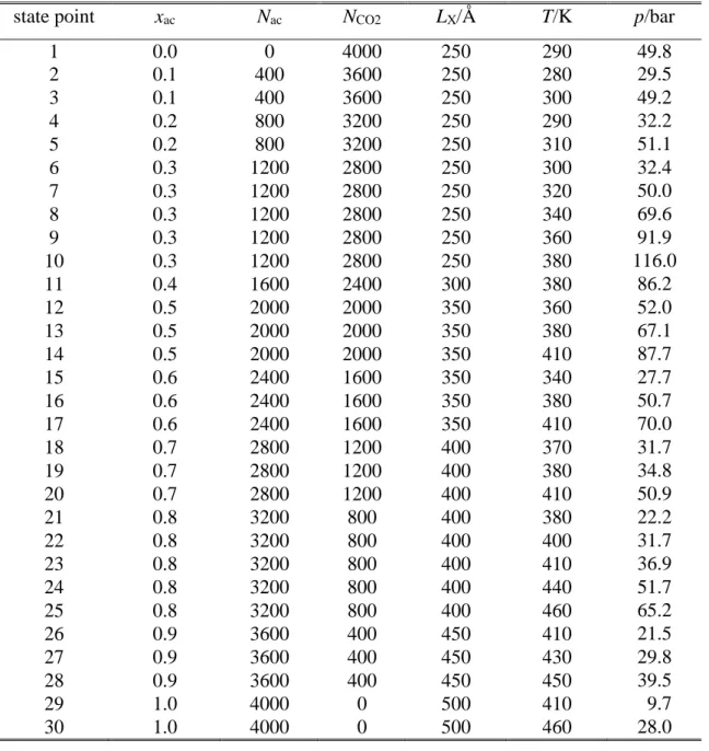
Table 1 Characteristics of the different systems simulated
state point xac Nac NCO2 LX/Å T/K p/bar
1 0.0 0 4000 250 290 49.8
2 0.1 400 3600 250 280 29.5
3 0.1 400 3600 250 300 49.2
4 0.2 800 3200 250 290 32.2
5 0.2 800 3200 250 310 51.1
6 0.3 1200 2800 250 300 32.4
7 0.3 1200 2800 250 320 50.0
8 0.3 1200 2800 250 340 69.6
9 0.3 1200 2800 250 360 91.9
10 0.3 1200 2800 250 380 116.0
11 0.4 1600 2400 300 380 86.2
12 0.5 2000 2000 350 360 52.0
13 0.5 2000 2000 350 380 67.1
14 0.5 2000 2000 350 410 87.7
15 0.6 2400 1600 350 340 27.7
16 0.6 2400 1600 350 380 50.7
17 0.6 2400 1600 350 410 70.0
18 0.7 2800 1200 400 370 31.7
19 0.7 2800 1200 400 380 34.8
20 0.7 2800 1200 400 410 50.9
21 0.8 3200 800 400 380 22.2
22 0.8 3200 800 400 400 31.7
23 0.8 3200 800 400 410 36.9
24 0.8 3200 800 400 440 51.7
25 0.8 3200 800 400 460 65.2
26 0.9 3600 400 450 410 21.5
27 0.9 3600 400 450 430 29.8
28 0.9 3600 400 450 450 39.5
29 1.0 4000 0 500 410 9.7
30 1.0 4000 0 500 460 28.0
Table 2 Interaction parameters of the potential models used
molecule interaction site /Å /kJ mol-1 q/e
acetone
CH3 3.790 0.8144 0
C 3.820 0.3324 0.424
O 3.05 0.6565 -0.424
CO2
C 2.800 0.2244 0.70
O 3.050 0.6566 -0.35
Table 3 Dynamical characteristics of the surface layer molecules.
state
point xac T/K res/psa D/Å2ps-1 b D/ps
acetone CO2 acetone CO2 acetone CO2
1 0.0 290 - 3.4 - 2.58 - 1.5
2 0.1 280 5.5 3.9 1.59 2.19 2.7 1.9
3 0.1 300 4.6 3.5 1.91 2.42 2.2 1.7
4 0.2 290 5.7 4.0 1.59 2.34 2.8 1.9
5 0.2 310 4.8 3.6 1.91 2.62 2.2 1.6
6 0.3 300 5.0 4.1 1.71 2.41 2.6 1.9
7 0.3 320 5.0 3.6 1.95 2.56 2.3 1.7
8 0.3 340 4.3 3.2 2.11 2.90 2.0 1.5
9 0.3 360 3.7 2.9 2.44 2.99 1.7 1.4
10 0.3 380 3.0 2.5 2.68 3.42 1.5 1.2
11 0.4 380 4.0 3.0 2.61 3.24 1.7 1.4
12 0.5 360 5.0 3.5 2.22 3.06 2.2 1.6
13 0.5 380 4.5 3.3 2.40 3.19 2.0 1.5
14 0.5 410 3.8 2.9 2.86 3.39 1.6 1.4
15 0.6 340 6.0 4.0 1.98 2.88 2.6 1.8
16 0.6 380 4.8 3.4 2.41 3.24 2.1 1.5
17 0.6 410 4.1 3.1 2.79 3.42 1.7 1.4
18 0.7 370 5.4 3.6 2.21 2.93 2.4 1.8
19 0.7 380 5.1 3.5 2.25 2.99 2.3 1.8
20 0.7 410 4.4 3.1 2.69 3.47 1.9 1.5
21 0.8 380 5.3 3.5 2.20 3.27 2.5 1.7
22 0.8 400 4.8 3.3 2.35 3.71 2.3 1.5
23 0.8 410 4.6 3.2 2.58 3.60 2.1 1.5
24 0.8 440 4.0 2.9 2.98 4.02 1.7 1.3
25 0.8 460 3.6 2.7 3.27 4.46 1.5 1.1
26 0.9 410 4.8 3.2 2.52 3.77 2.2 1.5
27 0.9 430 4.5 3.1 2.75 3.75 2.0 1.5
28 0.9 450 4.1 3.0 3.03 4.55 1.8 1.2
29 1.0 410 4.9 - 2.48 - 2.3 -
30 1.0 460 4.0 - 3.11 - 1.7 -
aError bars are in the order of 0.05 ps bError bars are below 0.05 Å2/ps
Figure legends
Fig. 1 Thermodynamic state points, shown on the T-p phase diagram, in which the liquid- vapour interface of the acetone-CO2 system is simulated. Different colours and symbols correspond to different overall composition of the system.
Fig. 2 Equilibrium snapshot of the surface portion of the systems of overall acetone mole fractions of 0.3 (left), 0.5 (middle), and 0.9 (right), as obtained at 380 K. Molecules pertaining to the first, second, third, and fourth molecular layers of the liquid phase are marked by red, green, blue, and orange colours, respectively, while those belonging to the bulk liquid and vapour phases are shown by purple and gray colours, respectively. Lighter shades correspond to the CO2, while darker shades to the acetone molecules.
Fig. 3 Mass density profile of the acetone (top panels) and CO2 (second panels) molecules, the entire system (third panels) and the surface layer of the liquid phase (bottom panels), as obtained in thermodynamic state points corresponding (a) to the overall acetone mole fraction of 0.8, (b) to the temperature of 410 K, and (c) to the pressure of 50 ± 2.5 bar. All profiles shown are symmetrized over the two interfaces present in the basic box.
Fig. 4 Mole fraction of the acetone molecules in the surface layer as a function of their mole fraction in the bulk liquid phase, as obtained in thermodynamic state points corresponding to the 380 K (red filled squares) and 410 K (green filled circles) isotherms, and to the 30 ± 2.5 bar (blue open squares) and 50 ± 2.5 bar (orange open circles) isobars. The lines connecting the points are just guides to the eye. The black straight line shows the bulk liquid phase acetone mole fraction for reference.
Fig. 5 Acetone mole fraction in the coexisting bulk liquid (green squares) and vapour (black circles) phases as well as in the surface layer of the liquid phase (red triangles), as obtained in thermodynamic state points corresponding to the pressure of 30 ± 2.5 bar (top panel) and to the temperature of 380 K (bottom panel). The lines connecting the points are just guides to the eye.
Fig. 6 Mass density profile of the CO2 (black solid lines) and acetone (red dashed lines) molecules belonging to the surface layer, as obtained in systems of the overall acetone mole fraction of 0.8 (top panel), 0.6 (middle panel), and 0.3 (bottom panel). All profiles shown are symmetrized over the two interfaces present in the basic box. Scales on at the left and right correspond to the density of the acetone and CO2 molecules, respectively. The inset shows a snapshot of the surface layer of the xac = 0.5 system, simulated at 360 K (side view). Centres of the acetone and CO2 molecules are shown by red and green balls, respectively.
Fig. 7 (a) Temperature and (b) pressure dependence of the reciprocal width of the surface layer, as obtained in thermodynamic states corresponding to (a) the same pressure or (b) temperature (top panels), and to the same overall acetone mole fraction (bottom panels). For states corresponding to the same overall acetone mole fraction, the straight lines fitted to the simulated data are also shown.
Fig. 8 Area distribution of the Voronoi cells of (a) the acetone, and (b) the CO2 molecules pertaining to the surface layer, as obtained, by disregarding the other component, in thermodynamic states corresponding to the overall acetone mole fraction of 0.3 (top panels), to the temperature of 380 K (middle panels), and to the pressure of 50 ± 2.5 bar (bottom panels). Simulation results are shown by symbols, while their best fitting gamma function (eq.
2) are shown by solid curves of the same colour. To emphasize the decay of their large area tails, the distributions are shown on a logarithmic scale. Voronoi cells have been calculated by projecting the molecular centres to the macroscopic plane of the interface, YZ.
Fig. 9 Instantaneous equilibrium snapshots of the systems corresponding to the overall acetone mole fraction of 0.3 (left), 0.5 (middle) and 0.8 (right), simulated at 380 K, showing the projection of the centres of the surface acetone (red circles) and CO2 (green circles) molecules to the macroscopic plane of the interface, YZ.
Fig. 10 (a) Definition of the local Cartesian frame fixed to the individual acetone molecules and of the orientational angles and , and , characterizing the alignment of the acetone and CO2 molecules, respectively, relative to the macroscopic surface normal vector, X, pointing, by our convention, from the liquid to the vapour phase. (b) Definition of the separate regions A, B and C of the surface layer through its density profile.