2010 / 5 W P

(1)

CORVINUS UNIVERSITY OF BUDAPEST

DEPARTMENT OF MATHEMATICAL ECONOMICS AND ECONOMIC ANALYSIS Fövám tér 8., 1093 Budapest, Hungary Phone: (+36-1) 482-5541, 482-5155 Fax: (+36-1) 482-5029 Email of the author: zsolt.darvas@uni-corvinus.hu

Website: http://web.uni-corvinus.hu/matkg

W ORKING P APER

2010 / 5

B EYOND THE C RISIS :

P ROSPECTS FOR E MERGING E UROPE

Zsolt Darvas

22 December 2010 (original version) 9 March 2011 (this revised version)

(2)

Beyond the crisis: prospects for emerging Europe

Zsolt Darvas 9 March 2011

Abstract

This paper assesses the impact of the 2008-09 global financial and economic crisis on the medium-term growth prospects of the countries of central and eastern Europe, the Caucasus and Central Asia, which began an economic transition about two decades ago. We use cross- country growth regressions, putting special emphasis on a proper consideration of the crisis and robustness. We find that the crisis has had a major impact on the within-sample fit of the models used and that the positive impact of EU enlargement on growth is smaller than previous research has shown. The crisis has also altered the future growth prospects of the countries studied, even in the optimistic but unrealistic case of a return to pre-crisis capital inflows and credit booms.

JEL: C31; C33; O47

Keywords: crisis; economic growth; growth regressions; transition countries This paper is forthcoming in Comparative Economic Studies

Acknowledgement: I am grateful to conference participants at the CICM Conference '20 Years of Transition in Central and Eastern Europe: Money, Banking and Financial Markets', the Tallinn University of Technology Conference 'Economies of Central and Eastern Europe:

Convergence, Opportunities and Challenges', and ECOMOD 2010, and seminar participants at Bruegel, the European Bank for Reconstruction and Development and the Vienna Institute for International Economic Studies for comments and suggestions. Without implicating him in any way, I would also like to thank Alessandro Turrini for his comments and suggestions.

Excellent research assistance by Maite de Sola, Juan Ignacio Aldasoro and Lucia Granelli is gratefully acknowledged as well as editorial advice from Stephen Gardner. Bruegel gratefully acknowledges the support of the German Marshall Fund of the United States to research underpinning this paper.

Zsolt Darvas is a Research Fellow at Bruegel, Rue de la Charité 33, 1210 Brussels, Belgium, e-mail: zsolt.darvas@bruegel.org He is also a Research Fellow at the Institute of Economics of the Hungarian Academy of Sciences, and Associate Professor at the Corvinus University of Budapest.

(3)

1. Introduction

Before the crisis, the countries of Central and Eastern Europe, the Caucasus and Central Asia (CEECCA)¹ seemed to be making rapid and reasonably smooth economic progress, following an extraordinarily deep recession after the collapse of the communist regimes. The development model of most CEECCA countries had many common features, such as deep political, institutional, trade and financial integration with the EU and significant labour mobility to EU15 countries. However, there were also substantial differences between countries, which became more notable in the run-up to the global crisis: in a few CEECCA countries catching up was generally accompanied by macroeconomic stability, but most countries of the region became increasingly vulnerable due to huge credit, housing and consumption booms, high current-account deficits and quickly rising external debt². It was widely expected even before the crisis that these vulnerabilities must be corrected at some point, but the magnitude of the corrections when they did happen were amplified by the global financial and economic crisis.

Beyond the crisis, a major question is if the crisis is likely to have lasting economic effects.

This paper assesses pre-crisis growth drivers and the medium term prospects of the CEECCA region using cross-country growth regressions, which estimate, in cross-section and panel regression frameworks, empirical relationships between growth and a number of potential growth drivers.

Many papers have adopted cross-country growth regressions for CEECCA countries; see for example Schadler et al (2006), Falcetti, Lysenko and Sanfey (2006), Abiad et al (2007), Vamvakidis (2008), Cihak and Fonteyne (2009), Iradian (2009), European Commission (2009), and Böwer and Turrini (2010), just to mention a few of the more recent papers.

However, all of these papers used sample periods that ended before the crisis and covered only the boom years of the 2000s, this boom proving unsustainable in many CEECCA

1 The CEECCA countries that formerly belonged to the political and economic sphere of the Soviet Union have a common historical root but are rather diverse. Ten countries are members of the European Union (Bulgaria, Czech Republic, Estonia, Hungary, Latvia, Lithuania, Poland, Romania, Slovakia and Slovenia). Seven countries in the western Balkan are either EU accession candidates or potential candidates (Albania, Bosnia and

Herzegovina, Croatia, the Former Yugoslav Republic of Macedonia, Montenegro, Serbia, and Kosovo under UNSC Resolution 1244/99, though we do not include Montenegro and Kosovo in our study due to lack of data).

Among the twelve other former Soviet Union countries five are major hydrocarbon exporters (Azerbaijan, Kazakhstan, Russia, Turkmenistan and Uzbekistan) while the other seven are not (Armenia, Belarus, Georgia, Kyrgyz Republic, Moldova, Tajikistan and Ukraine); most of these countries belong to the Commonwealth of Independent States (CIS) and we shall refer them accordingly. Mongolia is also a transition country, while Turkey – another EU candidate – is not, but we also include it in our study due to its geographical proximity.

2 See extensive analyses of the development model of the CEECCA region and assessments of its future potential in Bruegel and wiiw (2010), Cihák and Fonteyne (2009), Fabrizio et al (2009) and Mitra et al (2009).

(4)

countries. Pre-crisis unsustainable developments have also characterised a couple of advanced countries, like the US or some Mediterranean euro-area countries, yet to a lesser degree than in CEECCA. Other emerging and developing countries, however, were largely exempt from such developments. Pre-crisis vulnerabilities have likely contributed to the crisis response as well. In this regard it is important to emphasize that CEECCA countries have been hit harder by the crisis than advanced countries and other emerging and developing economies countries, and post-crisis recovery is also generally slower for CEECCA countries (Bruegel and wiiw, 2010). Making estimates for a sample period that proved to be unsustainable will obviously bias the results toward the finding of higher growth. When the sample includes mostly booming countries, the estimated relationships between growth and fundamentals are distorted. When the sample includes a large cross section of countries over a long time horizon, and the booming countries are in a minority, but are differentiated by a dummy, which is done in most of the literature, then the estimate of this dummy is likely biased upward. Therefore, even though the crisis-period data are also hardly representative of standard conditions and in most, if not all, countries the output gap turned to negative, including the bust phase of the economic cycle in the sample is necessary.

In our paper, we attempt a comprehensive consideration of the crisis and perform extensive robustness checks of cross-country growth regressions. To this end, we extend the sample period up to 2010, using more recent data up to 2009 and forecasts for 2010; the forecasts are primarily taken from the IMF‟s October 2010 World Economic Outlook and the January 2011 forecasts of the Economist Intelligence Unit. Our extended sample till 2010 also includes the beginning of the recovery from the crisis. The use of forecasts brings uncertainty to the estimates, but perhaps the possible errors in 2010 forecasts made in October 2010 and January 2011 are not so large, and since we use time-averaged data, the impact of the use of forecasts is bound to be small³. We perform the calculations both for the pre-crisis sample and for this extended sample period, studying the results for different country groups, different sample periods and a number of possible explanatory variables. We aim to answer the following three questions:

3 We should highlight that forecasts for many explanatory variables are not necessary because these explanatory variables represent initial conditions that lag some years compared to growth, though there are some

contemporaneous correlates as well. When it is only the regressand, the growth rate of GDP, which contains a measurement error due to the adoption of forecasts, it boosts the standard error of the estimate but does not distort the unbiasedness of the regression.

(5)

First, how much does the crisis alter the within-sample fit of cross-country growth regressions? We answer this question by presenting estimates for both the pre-crisis period ending in 2007 and for the full period ending in 2010 that also includes the crisis.

Second, has growth in CEECCA countries or of some sub-groups within this region been different from the rest of world in the sense that these countries grew more quickly than what would have been implied by their fundamental growth determinants? The literature has approached this question by studying the parameters of a dummy variable representing certain country groups in the growth regression. We also use this methodology and study the robustness of the estimated parameter of country group dummies in the context of the crisis.

But we also use a novel methodology to study the impact of EU enlargement on fundamentals. For the ten central and eastern European countries (CEE10) that joined the EU in 2004 and 2007 we set up a counterfactual scenario for the fundamentals such as capital inflows, trade integration and institutional development, under which no EU enlargement occurred, basing the scenario on the developments in non-EU middle income countries. We then use our estimated models to simulate the growth effects of the incremental improvement of fundamentals due to prospective and actual EU membership.

Third, how much has the crisis altered future GDP growth scenarios? The change in projections can be traced back to two factors: (1) change in the model and (2) change in the assumed path of explanatory variables. The econometric estimates provide an explanation for the first factor, and we shall formulate different scenarios for the second factor, drawing on the experience of previous crises.

We draw three main conclusions. First, the crisis has altered the within-sample fit of cross- country growth regressions. The downward revision of fitted values of GDP growth from the regressions is between one and three percent per year for most countries. Second, the positive impact of EU enlargement on growth is smaller than previous research has shown according to the point estimates, and even the point estimates are generally not statistically significant.

The dummy variable approach indicated that in the 2000s overall, the CEE10 countries seemed to grow only about 0.3 percent per year more than what would have been implied by their fundamentals, while the counterfactual simulation indicated about 0.15 percent per year extra growth because of the incremental improvement of fundamentals due to EU enlargement. Adding these two results, EU enlargement may have boosted economic growth by approximately half percent per year. However, since the output gap may have turned more

(6)

negative in CEE10 than in other countries of the world, these results may underestimate somewhat the positive impact of EU enlargement on growth in CEE10. And third, the crisis has also altered future GDP growth scenarios. Even in the optimistic scenario that assumes a return to the pre-crisis development of fundamentals, medium-term outlooks are below pre- crisis actual growth, especially in those countries that experienced substantial credit and consumption booms before the crisis.

The rest of the paper is organised as follows. Section 2 discusses our methodology and model selection issues. The results of the growth regressions are presented in section 3. We also answer our first research question in this section. Section 4 discusses the effect of EU enlargement on the growth of new EU member states and presents a discussion of the second research question. The third research question is analysed in section 5. Section 6 presents a summary.

2. Methodology and model selection issues 2.1 Sample

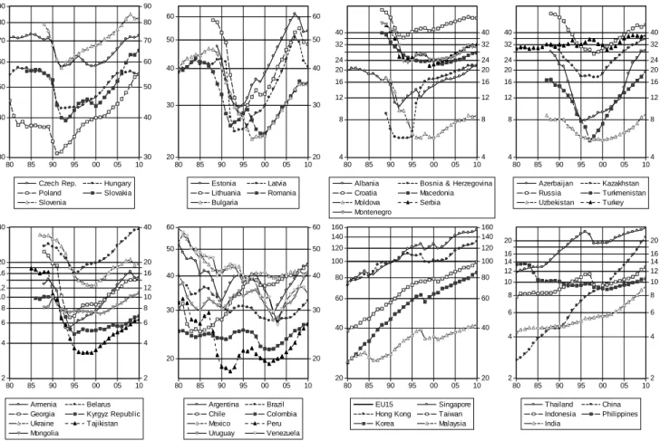
The execution of cross-country growth regressions typically involves a large degree of discretion. One issue is related to the length of the sample period: the longer the sample, the more precise the estimate, provided that there are no structural breaks. However, the pre- transition developments, when CEECCA countries operated under different economic systems, and the first years of transition, when these countries introduced market-oriented reforms and experienced extensive structural change, are not informative for current growth prospects because of significant structural breaks. Consequently, it is rather difficult to set an appropriate start date for the sample period. Figure 1 shows GDP per capita at purchasing power parity compared to the EU15 for the countries we study, in comparison to some Latin American and Asian countries for 1980-2010. Figure 1 clearly shows the extraordinarily deep recession that accompanied the first years of transition, but also the quick catching-up that followed in most countries, which can partly be regarded as a kind of reconstruction after the deep recession⁴. The recession lasted for just a few years in the case of the CEE10 countries

4 It was widely expected that countries undergoing transition would experience an initial decline in output and employment, but the depth and the length of the post-communist recession were unexpected (Fischer, 2002;

Svejnar 2006). The literature has proposed various explanations for this phenomenon. Svejnar (2006) categorises them into six main themes. First, a disorganisation among suppliers, producers and consumers associated with the central planning; second, the dissolution in 1990 of Comecon (Council for Mutual Economic Assistance), which governed trade relations across the Soviet bloc; third, difficulties of sectoral shifts in the presence of labour market imperfections; fourth, a switch from controlled to uncontrolled monopolistic structures in these economies; fifth, a credit crunch stemming from the reduction in state subsidies to firms and rise in real interest rates; and finally, tight macroeconomic policies may have played a role in the depth and length of the recession.

(7)

and some south-eastern European countries, but in most Commonwealth of Independent States (CIS) countries it lasted longer. Both the recession and the reconstruction period complicate the selection of a start date for the sample period.

Another issue is whether or not the sample should include panel data at a yearly frequency, time-averaged data over non-overlapping intervals, or time-averaged pure cross-section data.

The advantage of a cross-section setup is that issues related to dynamic panels do not arise and endogeneity is less of a concern, though causality cannot be claimed unless suitable instruments are found.

Figure 1: GDP per capita at purchasing power parity (EU15=100), 1980-2010

90 80 70 60

50

40

30

90 80 70 60

50

40

30

80 85 90 95 00 05 10

Czech Rep. Hungary

Poland Slovakia

Slovenia

60

50

40

30

20

60

50

40

30

20

80 85 90 95 00 05 10

Estonia Latvia Lithuania Romania Bulgaria

40 32 24 20 16 12 8

4

40 32 24 20 16 12 8

4

80 85 90 95 00 05 10

Albania Bosnia & Herzegovina Croatia Macedonia

Moldova Serbia

Montenegro

40 32 24 20 16 12 8

4

40 32 24 20 16 12 8

4

80 85 90 95 00 05 10

Azerbaijan Kazakhstan Russia Turkmenistan Uzbekistan Turkey

40

20 16 12 10 8 6 4

2

40

20 16 12 10 8 6 4

2

80 85 90 95 00 05 10

Armenia Belarus Georgia Kyrgyz Republic Ukraine Tajikistan Mongolia

60 50

40

30

20

60 50

40

30

20

80 85 90 95 00 05 10

Argentina Brazil

Chile Colombia

Mexico Peru

Uruguay Venezuela 160 140 120 100 80 60

40

20

160 140 120 100 80 60

40

20

80 85 90 95 00 05 10

EU15 Singapore

Hong Kong Taiwan

Korea Malaysia

20 16 14 12 10 8 6

4

2

20 16 14 12 10 8 6

4

2

80 85 90 95 00 05 10

Thailand China Indonesia Philippines India

Source: Author‟s calculation based on data from IMF World Economic Outlook April 2010 and EBRD.

The selection of the country sample is another key issue. The very reason behind cross- country regressions is that the countries in the sample share similar characteristics; when many countries are included, the country-specific factors or the effects of randomness on the results could be lessened. However, certain countries may have significantly different characteristics and the same factors may have different effects on growth. For example,

(8)

exclusion of very small countries can be justified on the basis that their economies could be less diversified and hence could be affected more strongly by particular shocks related to their main business activity. The level of a country's development also has an important bearing on growth drivers and therefore the exclusion of both poor and rich countries can be justified⁵. Since results can be sensitive to the specific choices made with respect to the sample along the aspects we have discussed, we use different sample periods that all start well after the collapse of communist regimes and study different country samples. In particular, we use three different time periods: cross section data for 2000-07; cross section data for 2000-10;

panel data with three non-overlapping five-year periods between 1995-2010. This latter sample has the advantage that it also includes some major emerging-market crisis episodes of late 1990s. We use four different country samples that are constrained by data availability only: all countries of the world; countries with population above 1 million; middle-income countries with population above 1 million, ie., GDP per capita at PPP compared to the US between 12.5 percent and 67.4 percent; and CEECCA countries only⁶.

2.2 Selection of variables and model design

A crucial issue is the selection of variables. This can also be subject to a large degree of discretion, because there are many indicators that can be used to measure a certain factor that are more or less correlated. The actual results may be sensitive to the selection of the variables used. Few authors acknowledge as honestly as Berg et al (1999) that results could be sensitive to model selection: “In other words, the same dataset could be used to make contradictory claims about the significance or lack of significance of various policy variables. Ad-hoc regressions of growth on a small number of policy variables, abundant as they are in the literature, thus deserve skepticism.” (p52). In a seminal article, Levine and Renelt (1992) find in a growth regression framework that very few economic variables are robustly correlated with economic growth rates. They could only detect positive and robust correlation between average growth rates and two variables: the investment rate (share of investment in GDP) and trade openness (the share of trade in GDP). But they could not detect robust correlation for a

5 See Veugelers (2010) for a discussion of the different role of various factors for technological progress along the development path.

6 The cut-off values for the third country group, which are based on the average GDP per capita at PPP compared to the US in the 2000-10 period, were determined on the basis of CEE10 countries. We calculated their

minimum, 23.0 percent for Bulgaria, and maximum, 56.9 percent for Slovenia, and the standard deviation, which was subtracted from the minimum and added to the maximum to determine a possible range. However, we also include in this middle-income country group those seven CIS countries that have lower per capita income, as well as Mongolia, in order to be able to analyse all CEECCA countries using the same model.

(9)

broad array of other potential explanatory variables. The extensive survey presented in Durlauf, Johnson and Temple (2005) broadly confirms these findings and concludes that

“growth econometrics is an area of research that is still in its infancy” (p. 651).

When we have looked for a single best model, we have indeed found considerable sensitivity to the time period, the country sample and the set of explanatory variables, which is in line with the findings of Levine and Renelt (1992), Berg et al (1999) and the literature survey of Durlauf, Johnson and Temple (2005)⁷. We try to overcome these issues by analysing different sample periods and country samples as discussed in Section 2.1 and using various explanatory variables to form different models. We run many regressions, each of which are „acceptable‟

in a sense that we will discuss shortly. We then report the distribution of estimates from various models, which also serves as a robustness check.

Considering the variables to be analysed, initial GDP per capita at purchasing power parity (PPP) was found in the literature to be the most robust explanatory variable and we of course also include it, having found that it is indeed a robust explanatory variable. We have also considered variables that are frequently used in the empirical growth literature, including the two variables that were found robust by Levine and Renelt (1992), such as the investment rate, trade openness, educational indicators, the dependency ratio, population growth, inflation, fiscal balance, research and development expenditures, patents and variables related to financial and institutional development. Some of these variables are related to the key pillars of the development model of most CEECCA, which are of special interest.

The four key pillars of the development model of most CEECCA countries were financial, trade and institutional integration with the western world and labour mobility⁸. We have therefore employed the following variables related to these factors. First, concerning financial integration, we used inward FDI per GDP (both stock and inflow), investment rate (gross fixed capital formation over GDP) and stock and change in private sector credit/GDP.

Different theories argue whether the stock or flow of certain financial variables, like FDI,

7 Multicollinearity among some variables may also explain the difficulties in finding a single best model. Note that multicollinearity affects the parameter estimates and their standard errors, but it does not reduce the predictive power or reliability of the model as a whole.

8 There are clear differences within the CEECCA region, however. The CEE10 have reached the highest level of integration, followed by the countries of the western Balkans that have either EU „candidate‟ or „potential candidate‟ status. The six „Eastern Partnership‟ countries, which were part of the Soviet Union, have reached a varying degree of integration with the EU15, while integration was generally minor for most of the other former Soviet Union countries.

(10)

matters, and for pragmatic reasons we included both. Second, regarding foreign trade we used trade openness measured as exports plus imports over GDP, the change in the terms of trade and share of fuel and food in total exports. Third, as to institutional development, we used the governance indicators complied by the World Bank, Transparency International's corruption perception index and a couple of the indicators compiled by Economic Freedom Network.

And fourth, for migration we used remittances over GDP⁹.

We also introduced a new variable that we have termed GDP historical gap to measure the ratio of a country‟s comparative output, measured by its current GDP per capita at PPP compared to the US, to the country‟s maximum comparative output in the past. The intuition is that countries that were closer to the US at a point in time in the past may have a better chance to catch up than other countries with similar fundamentals, because catching-up in this case implies reaching a level that has already been reached in the past. This variable has a low value after a crisis, such as the economic collapse during the first years of transition. This variable is applied to all countries in the sample, not just to CEECCA countries, and considers data since 1980¹⁰. Among our main country groups, the CIS countries still score low in this measure as they have not yet reached their pre-transition levels compared to the US¹¹.

This way we have established a set of 34 possible explanatory variables in addition to initial GDP per capita. Of this set, we first identified potential growth drivers and correlates in the following way. We adopted the three temporal samples and four country samples discussed is Section 2.1, ie, 12 samples altogether, and estimated cross-section and panel regressions, including constant and initial GDP per capita at PPP, as well as period fixed effects for the panels. We always controlled for initial GDP per capita at PPP because this variable proved to be the most robust variable in practically all cross-country growth regressions. We included only one other possible growth determinant of the 34 variables at a time. When a variable had a correctly signed, judged from economic principles, and significant parameter estimate in most of the 12 samples, we regarded it as a useful candidate for the growth regressions.

9 Unfortunately, it is difficult to collect reliable data on migration for a wide range of countries and time periods.

10 For most CEECCA countries the available data starts in 1989 with the exception of a few, for which data for earlier years is also available.

11 Falcetti et al (2006) and Iradian (2009) use a discrete dummy variable to measure the same phenomenon. The dummy takes a value of 1 if output in a given year is below 70 percent of its 1989 value. Böwer and Turrini (2010) adopt a continuous variable to capture this effect and hence it is the closest to our variable: they define an 'output loss' variable as the ratio of current output to the average output during 1990-95.

(11)

Using this methodology, we have selected 14 of the 34 variables considered¹². When selecting the variables we aim for balance; that is, we do not want to over-represent any particular kind of indicator, such as institutional quality, for which many variants tend to correlate well with GDP growth. We selected seven initial conditions: GDP historical gap, secondary school enrolment, dependency rate, legal system and property rights, freedom of trade, share of fuel exports, and the stock of inward FDI/GDP. We also selected seven contemporaneous correlates: investment/GDP, exports plus imports/GDP, population growth, fiscal balance/GDP, change in the terms of trade, growth in credit to private sector/GDP, and FDI inflow/GDP.

The inclusion of contemporaneous correlates obviously raises the issue of endogeneity, which could be handled, for example, by properly-selected instruments. However, the selection of good instruments is rather difficult if not impossible. For example, Iradian (2009) used a set of instruments for the reform indexes, such as the distance to Brussels, the share of commodity exports as percent of total export, and some others, but for other endogenous variables, such as fiscal balance, investment rate or inflation, he could not assemble suitable instruments. We have reviewed many papers in the literature that could not find proper instruments. A mechanical use of the lags of endogenous variables, a procedure frequently adopted in the literature, is not an appropriate solution either. Furthermore, Stock, Wright and Yogo (2002) demonstrated that the possible adoption of weak instruments renders conventional instrumental-variable inferences misleading. Hauk and Wacziarg (2009) studied bias properties of estimators commonly used to estimate growth regressions with Monte Carlo simulations and concluded that the simple OLS estimator applied to a single cross-section of variables averaged over time performed the best. For all these reasons we do not use instrumental variables, but apply OLS. This implies that we cannot interpret our results in a causal way, eg., higher investment leads to higher growth; rather, the interpretation of the relationship as a correlation is sufficient for our purposes.

Having selected 14 potential variables, we run growth regressions with all possible quartets (ie 4-element subsets) of the 14 variables. There are 1001 such quartets. Our initial conditioning variable, GDP per capita compared to the US, is always included, as well as time-period fixed effects for the panels. In the next sections, which study the three questions we raised in the introduction, we report the whole distribution of the growth estimates from

12 See detailed results of this exercise in Table 1 of Darvas (2010b).

(12)

the 1001 regressions. In the estimations we shall concentrate on our third country sample, 66 middle-income countries with population above 1 million.

3. How much does the crisis alter the within-sample fit of cross-country growth regressions?

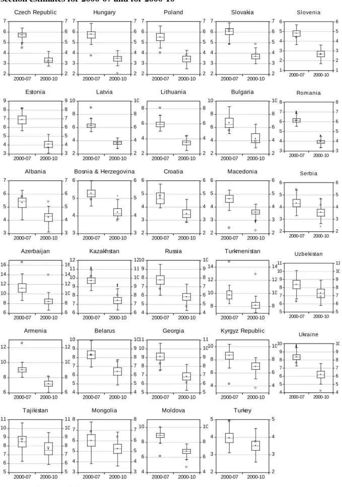
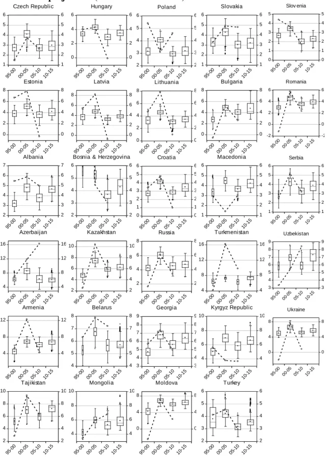
Following the model specification steps discussed in the previous section, we ran the 1001 cross-country growth regressions for two cross-section sample periods: the sample covering the pre-crisis „boom years‟ only (2000-07) and the sample which also includes the bust and the beginning of the subsequent recovery (2000-10). Figure 2 shows actual average GDP growth and the distribution of the in-sample fit derived from the 1001 cross-section regressions. The distribution is presented in the form of a box-plot (see the note to the figure for details).

The main message of the figure is the sizeable downward revision from the 2000-07 sample to the 2000-10 sample of both actual growth and fitted values of growth from the regressions.

For most countries the downward revision is between one and three percent per year. In some cases, actual growth fits well with the distribution of the 1001 estimates, but there are outliers.

We would like to highlight, however, that the goal was not find a perfect fit for all countries but to estimate models that can be used to assess the potential rate of growth.

For example, in the cases of Estonia, Latvia and Lithuania, actual growth was well above the distribution of estimates in the 2000-07 period. When the sample is extended till 2010, however, the actual growth of Estonia and Latvia fall within the interquartile range of the distribution of 1001 fitted values of growth from the regressions and is not far from the range in the case of Lithuania. Consequently, our calculations indicate that the three Baltic countries grew above their potential in the pre-crisis period, which has likely contributed to the huge current-account deficits of these countries, but considering the whole 2000s, average growth may not have been far from potential.

Azerbaijan and Turkmenistan, two oil exporters, provide a different example as actual growth turned out to be much higher than fitted by our model before the crisis and in the sample period that also includes crisis. Although the terms of trade and the share of fuel exports in total exports are included in our models, it seems that none of the models could capture the past growth processes in Azerbaijan and Turkmenistan. Armenia also had extremely rapid growth in 2000-07 that our models cannot explain.

(13)

Figure 2: The effect of the crisis on in-sample fit from 1001 growth regressions: cross section estimates for 2000-07 and for 2000-10

2 3 4 5 6 7

2000-07 2000-10 Czech Republic

3 4 5 6 7 8 9

2000-07 2000-10 Estonia

3 4 5 6 7

2000-07 2000-10 Albania

6 8 10 12 14 16

2000-07 2000-10 Azerbaijan

6 8 10 12

2000-07 2000-10 Armenia

5 6 7 8 9 10 11

2000-07 2000-10 Tajikistan

2 3 4 5 6 7

2000-07 2000-10 Hungary

2 4 6 8 10

2000-07 2000-10 Latvia

3 4 5 6

2000-07 2000-10 Bosnia & Herzegovina

6 7 8 9 10 11 12

2000-07 2000-10 Kazakhstan

4 5 6 7 8 9 10

2000-07 2000-10 Belarus

3 4 5 6 7 8

2000-07 2000-10 Mongolia

2 3 4 5 6 7

2000-07 2000-10 Poland

2 4 6 8

2000-07 2000-10 Lithuania

2 3 4 5 6

2000-07 2000-10 Croatia

4 5 6 7 8 9 10

2000-07 2000-10 Russia

5 6 7 8 9 10 11

2000-07 2000-10 Georgia

4 6 8 10

2000-07 2000-10 Moldova

2 3 4 5 6 7

2000-07 2000-10 Slovakia

2 4 6 8 10

2000-07 2000-10 Bulgaria

2 3 4 5 6

2000-07 2000-10 Macedonia

8 10 12 14

2000-07 2000-10 Turkmenistan

4 6 8 10

2000-07 2000-10 Kyrgyz Republic

2 3 4 5

2000-07 2000-10 Turkey

1 2 3 4 5 6

2000-07 2000-10 Sl oveni a

3 4 5 6 7 8

2000-07 2000-10 Rom ani a

2 3 4 5 6

2000-07 2000-10 Serbi a

5 6 7 8 9 10 11

2000-07 2000-10 Uzbeki stan

4 5 6 7 8 9 10

2000-07 2000-10 Ukrai ne

Source: Author‟s calculations.

Note. Empty circle: actual annualised (compounded) GDP growth over the five-year period. The box-plots show the empirical distribution of the in-sample fit of 1001 regressions. Note also that each individual fit has its own confidence band. The dependent variable is the average annualised real GDP growth (in percent) during the

(14)

period shown on the horizontal axis. All regressions include the initial GDP per capita at PPP compared to the US and three regional dummies (10 new EU member states; six western Balkan countries; 12 CIS countries) as explanatory variables. The 1001 regressions comprise all possible quartets of the remaining fourteen explanatory variables.

The box-plot represents the distribution of the fits (point estimates) derived from the regressions. The box portion of a box-plot represents the first and third quartiles (middle 50 percent of the estimates, which is called the interquartile range), the median is depicted using a line through the centre of the box, while the mean is drawn using a filled circle. The whiskers and staples ('error bars') show the values that are outside the first and third quartiles, but within 1.5 times the interquartile range (ie 1.5 times the difference between first and third quartiles). Outliers, if any, are indicated with separate symbols outside the staples. Box widths are proportional to number of feasible regression fits, which is 1001 in this figure; but in Figure 4 some of parameter estimates and in Figure 7 some of the regression fits and projections could not be calculated due to missing data.

Hungary presents a different picture since actual growth is below the level of growth predicted by the model in both sample periods. This finding could be explained by the fact that GDP growth had already slowed down in the mid-2000s partly due to domestic policies such as fiscal austerity to eliminate the nearly double digit, as a percentage of GDP, budget deficit of 2002-06, and partly due to structural weaknesses. The country may have therefore grown below potential already before the crisis. Macedonia also had a disappointing growth performance, which was not just below the fitted values of growth from our regressions, but was also below the growth rates of all other countries of the region. Domestic factors, which are not included in our model, were presumably responsible for this.

In the cases of most other countries actual growth falls within the interquartile range of the fitted growth from the regressions especially in the 2000-10 sample. This suggests that growth during the whole decade of the 2000s could be more in line with fundamentals than growth during the 2000-07 period.

4. How large is the impact of EU accession on growth in CEE10?

EU accession can directly improve the fundamentals that drive economic growth, such as higher capital inflows, higher trade flows, a better legal environment, etc, but can also have a growth dividend beyond the effects of enlargement on the fundamental determinants of growth. This dividend can be due to, for example, enhanced credibility, which is not captured by any other variable included in the model. To our knowledge, earlier papers that have adopted growth regressions have only considered this second factor using dummy variable approaches, which we also use in Section 4.1. But in Section 4.2 we consider as well the first factor using a counterfactual simulation.

(15)

4.1 Dummy variable approach

It is common practice to include regional dummies in cross-country growth regressions.

When the estimated parameter of such a dummy is significantly greater then zero, one may argue that the country group under consideration grew faster than what would have been implied by the countries' fundamental growth determinants. For example, the European Commission (2009) reports the result, based on the detailed analysis of Böwer and Turrini (2010), that EU enlargement contributed to 1.75 percent excess annual growth in every year between 2000 and 2008 of the CEE10 countries beyond the effects of enlargement on the fundamental determinants of growth. This result was obtained from a panel regression in which a dummy variable was added to the growth performance of the CEE10 states for the 2000-08 period¹³. Although CEE10 joined the EU between 2004 and 2007, it is rightly assumed that the positive impact of EU admission already had an impact before the actual date of joining; thereby the year 2000 seems a reasonably starting year. Regarding CIS countries, Åslund and Jenish (2006) found that these countries had exhibited extraordinary growth performance since 2000. As we have argued in the introduction, these and all other estimates for sample periods ending before the crisis are likely biased upwards because they were based on the period of fast growth covering only the boom part of the 2000s, which proved to be unsustainable for many CEECCA countries, but not in most other emerging and developing countries. We now study the impact of the sample period on the results.

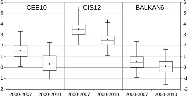
To start, we estimated our 1001 regressions as pure cross-section models for growth from 2000 until 2007 and for a longer period ending in 2010. Figure 3 plots the distribution of the parameter estimates of three regional dummies of CEECCA countries. The estimated parameter of the dummy for the new EU member states is found to be positive in the pre- crisis period and the 1.75 percentage point estimate of the European Commission (2009) and Böwer and Turrini (2010) fits well within the distribution. But considering the whole 2000s, the parameter estimates of the dummy are much lower. The mean of the 1001 estimates is positive and correspond to a 0.3 percent annual growth dividend, but zero is included in the interquartile range and the median is very close to zero.

Regarding the CIS countries, Figure 3 suggests that their growth rate was indeed higher than what would have predicted by fundamentals, considering both the pre-crisis period and the full sample, though the estimates are somewhat lower in the full period. The dummy

13 The sample period of Böwer and Turrini (2010) covers actual data till 2007 and the spring 2008 forecast of the European Commission for 2008.

(16)

representing western Balkan countries has mostly positive parameter estimates in the 2000- 2007 sample, but in the 2000-2010 sample the parameter estimates are almost symmetrically distributed around zero.

Figure 3: Distribution of the parameter estimates of the regional dummies from 1001 cross section regressions: comparison of the 2000-07 and 2000-10 cross-section samples

-2 -1 0 1 2 3 4 5 6

2000-2007 2000-2010 2000-2007 2000-2010 2000-2007 2000-2010

CEE10 CIS12 BALKAN6

Note. The figure shows the empirical distribution of the parameter estimates of the three regional dummies from 1001 different regressions in the form of box-plots. See the note to Figure 2 on the interpretation of the box-plot.

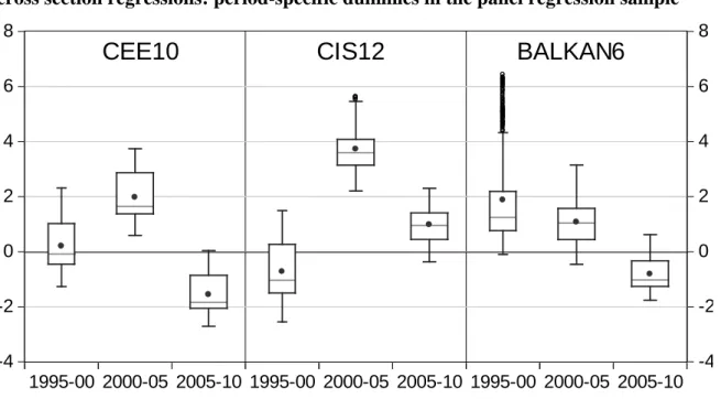
To further test the time profile of country group dummy parameters, we estimated the models in a panel setup with five-year non-overlapping periods in 1995-2010 and allowed the parameter of the country group dummy to change over time. Results are shown in Figure 4.

The new EU member states grew above their fundamentals from 2000 to 2005 and below from 2005 to 2010. The magnitudes are similar to our previous estimates: the excess growth in 2000-05 was estimated to be around two percent per year with a median of 1.65, which is again very much in line with the findings of the European Commission (2009) and Böwer and Turrini (2010). During the second half of the 2000s, however, the growth performance of this country group is worse than in other countries of the world when controlling for fundamentals; hence, during the 2000s overall, the new member states do not differ from other countries. Similar conclusions can be drawn for the western Balkan countries, while the CIS countries still grew faster than was explained by the models during the 2000s, though their advantage has declined.

(17)

Figure 4: Distribution of the parameter estimates of the regional dummies from 1001 cross section regressions: period-specific dummies in the panel regression sample

-4 -2 0 2 4 6 8

1995-00 2000-05 2005-10 1995-00 2000-05 2005-10 1995-00 2000-05 2005-10

CEE10 CIS12 BALKAN6

Note. The figure shows the empirical distribution of the parameter estimates of the three regional dummies (included as three separate dummy variables for the three time periods of the panel) from 1001 different regressions in the form of box-plots. See the note to Figure 2 on the interpretation of the box-plot. The large number of outliers of the Balkan dummy for the 1995-2000 period are most likely due to Bosnia and Herzegovina, as the country had a very high growth, averaging 29.5 percent per year, following the Balkan war;

see the third panel of Figure 1. 286 of the 1001 regression cannot be estimated for the full 1995-2010 period due to missing data. We therefore estimated the models for two sample periods: for 1995-2010 (that includes three 5- year long periods) and for 2000-2010 (that includes two 5-year long periods). The estimates for 1995-2000 come from the first estimation, which was feasible for 715 regressions, while the estimates for 2000-2005 and 2005- 2010 from the second sample period, which was feasible for all the 1001 regressions.

4.2 Counterfactual simulation

We use a novel different approach as well to assess the growth impact of EU accession. We set up a counterfactual scenario for the fundamentals under which no EU enlargement occurred, basing the scenario on the development of non-EU middle income countries.

Among the 14 variables selected in Section 3, eight have likely been affected by EU accession: inflow of FDI, stock of FDI, credit to the private sector, foreign trade, investment, fiscal balance, freedom-of-trade index and the index for legal systems and property rights. We assume that EU accession did not have an effect on five variables: population growth, secondary school enrolment, dependency rate, share of fuel exports and the terms of trade.

The fourteenth variable, GDP historical gap, is affected indirectly by GDP growth.

(18)

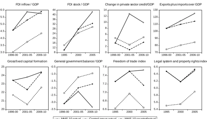
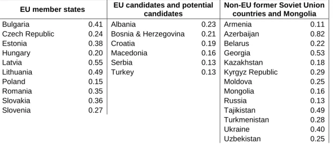
We have set up the counterfactual scenario for the fundamentals based on the development of 44 non-EU middle income countries¹⁴. To this end, we calculated the country-group average of the eight variables for the CEE10 and for the control group and assumed under the hypothesis of no EU enlargement that the change in the variables of the CEE10 compared to their pre-2000 values would have been identical to the change in the same variables of the control group. We used our panel regression sample covering three non-overlapping five-year periods between 1995 and 2010. Figure 5 shows, for the group averages, the actual developments in CEE10 the actual developments in the control group, and the counterfactual scenario for the CEE10. The assumed impact of EU enlargement on these fundamentals is shown by the difference between the actual and the counterfactual, ie, between the solid line with the circle and the dashed line. We applied these average impacts to each individual CEE10 countries.

Figure 5: Counterfactual scenario for eight variables of the CEE10 countries under no EU accession

3.0 3.5 4.0 4.5 5.0 5.5 6.0

1996-00 2001-05 2006-10 FDI inflow / GDP

8 12 16 20 24 28 32 36 40 44

1995 2000 2005

FDI stock / GDP

0 2 4 6 8 10 12 14

1996-00 2001-05 2006-10 Change in private sector credit/GDP

70 80 90 100 110 120 130

1996-00 2001-05 2006-10 Exports plus imports over GDP

20 21 22 23 24 25

1996-00 2001-05 2006-10 Gross fixed capital formation

-3.5 -3.0 -2.5 -2.0 -1.5 -1.0 -0.5

1996-00 2001-05 2006-10 General government balance / GDP

6.6 6.8 7.0 7.2 7.4 7.6

1995 2000 2005

NMS-10 actual Control group actual NMS-10 counterfactual Freedom of trade index

5.4 5.6 5.8 6.0 6.2 6.4 6.6

1995 2000 2005

Legal system and property rights index

Source: Author‟s calculations. See details in the main text.

Note. We assumed that EU accession had an impact on the development of variables after 2000. Consequently, for contemporaneous correlates the counterfactual scenario differs from the actual data during 2001-05 and

14 The income thresholds we applied were defined in Section 2. We did not include the four EU15 countries falling within the thresholds (Greece, Italy, Portugal and Spain). The 44 countries are: Albania, Algeria, Argentina, Azerbaijan, Belarus, Bosnia/Herzegovina, Botswana, Brazil, Chile, Colombia, Costa Rica, Croatia, Dominican Republic, Ecuador, El Salvador, Gabon, Iran, Israel, Jamaica, Kazakhstan, South Korea, Lebanon, Libya, Macedonia, Malaysia, Mauritius, Mexico, Namibia, New Zealand, Oman, Panama, Peru, Russia, Saudi Arabia, Serbia, South Africa, Taiwan, Thailand, Trinidad and Tobago, Tunisia, Turkey, Ukraine, Uruguay, and Venezuela.

(19)

2006-10, while for initial conditions the 2005 values are different. Note that dependent variable of the regressions it the average annualised growth from the beginning to the end of the 5-year long period, eg from 2000 until 2005, that is, during five years. Therefore, initial conditions from the year 2000 will be used, while contemporaneous correlates will be averaged for the same period as GDP growth, ie the average between 2001 and 2005 in the case of the 2000-2005 period. Note also that the FDI inflow is an average annual data and it is consistent with the development of the stock of FDI, as the stock is also influenced by valuation changes.

For example, in the counterfactual scenario under which no EU enlargement occurred, average annual FDI inflow/GDP would have been 5.3 percent instead of 5.9 percent in 2001- 05 (ie EU enlargement has resulted in more FDI inflows which boosted growth) and 5.9 percent instead of 5.8 percent in 2006-10 (almost neutral impact). The figure suggests that for most variables, EU accession has led to growth-enhancing development of the fundamentals (ie the actual outcome is above the counterfactual). The index for legal systems and property rights would have been broadly similar under the counterfactual scenario. It is only the fiscal balance that would have been better (and therefore growth enhancing) under the counterfactual scenario, suggesting that EU accession may have loosen the fiscal constrain.

We then use the estimated panel models to simulate the growth effects of the incremental improvement of fundamentals due to EU enlargement by calculating the difference between two simulations of all 1001 models. The first simulation uses actual data for all variables, while the second simulation uses the counterfactual values of the eight variables, as discussed above, and actual data for the other variables. Table 1 shows the distribution of the results.

The mean of the estimates is 0.15 percentage point per year and zero is not included in the interquartile range, though close to its boundary.

Table 1: The growth effects of the incremental improvement of fundamentals in the CEE10 states due to EU enlargement (percent)

2000-2005 2005-2010

Max 0.77 0.73

Upper 25% 0.19 0.27

Mean 0.14 0.15

Lower 25% 0.01 0.01

Min -0.03 -0.22

Note. Values show the distribution of 1001 estimates for the effects of the incremental improvement of fundamentals due to EU enlargement on annual real GDP growth, which were derived as the difference between two simulations: one using actual data and one using counterfactual values for eight variables under the hypothesis of no EU enlargement for the CEE10 states. See details in the main text.

(20)

Taken together, the results of the dummy variable approach and the counterfactual simulation approach show a positive impact of EU enlargement on growth in the CEE10 states, considering even the full decade of the 2000s, but the results are much smaller than previous research has found for the pre-crisis sample and are generally not significant. The dummy variable approach, which measures the impact of EU enlargement above the impact of EU enlargement on fundaments, suggested a point estimate around 0.3 percent per year. The counterfactual simulation, which measures the impact of EU enlargement through better fundamentals, suggested 0.15 percent per year. Therefore, these two complementary methods together suggest about 0.45 percent per year extra growth in CEE10 due to EU enlargement.

5. Post-crisis growth prospects

Finally, we study prospects for post-crisis growth using our estimated models and by setting up hypothetical scenarios for the future development of growth drivers, using our models estimated on the panel regression sample of 1995-2010. Based on the findings discussed in the previous section, we allow a country group dummy variable only for the CIS group in our estimated models. Since the parameter of the period CIS dummy declined in the second half of the 2000s, and we do not want to pick this last estimate because it may be sensitive to the effects of the crisis, we include a single CIS dummy for the whole 1995-2010 period.

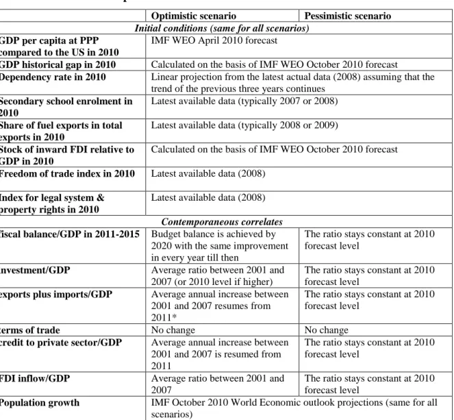
For the projections for 2011-15, we have set up three scenarios, optimistic, pessimistic and an intermediate. For the optimistic scenario, we assume that pre-crisis developments will resume, so that for most variables the average changes from 2000 to 2007 are extrapolated using the 2010 starting values. For the pessimistic scenario, we assume that capital inflows will be permanently reduced, foreign trade and domestic credit will expand only in line with GDP, the investment rate will stabilise at the 2010 level and the budget balance will not improve after 2010. Table 2 details the assumptions behind these two scenarios. For the intermediate scenario, we assume that the key variables take the average of their values in the optimistic and pessimistic scenarios. The period fixed effects, which are included in the panel regression, are assumed to be zero for 2010-15.

However, in the following cases the optimistic scenario turned to be worse than the pessimistic scenario and therefore we have corrected for that. First, Turkmenistan and Uzbekistan had a budget surplus in 2010 and therefore our assumption of reaching a balanced budget by 2020 would deteriorate the balance. For these two countries we assumed the stability of the 2010 budget surplus in all scenarios. Second, also in Turkmenistan and

(21)

Uzbekistan the credit/GDP ratio was falling before the crisis, but our optimistic scenario should not assume a continued fall. We have therefore assumed that in the optimistic scenario credit growth will be the same used the average of Armenia, Belarus, Georgia, Kyrgyzstan, Ukraine and Tajikistan. Third, in eight countries (Armenia, Belarus, Bosnia and Herzegovina, Estonia, Kazakhstan, Russia, Tajikistan, Turkmenistan and Ukraine) trade openness would be lower in the optimistic than in the pessimistic scenario and therefore for these countries we assumed the constancy of the 2010 ratio in all scenarios. And finally, for five countries (Albania, Armenia, Belarus, Mongolia and Uzbekistan) FDI inflow/GDP would be less in our optimistic scenario and therefore we have also used the 2010 value in all scenarios. These adjustments imply that the difference between the optimistic and the pessimistic projections is bound to be less for these countries.

Table 2. Detailed assumptions of the scenarios

Optimistic scenario Pessimistic scenario Initial conditions (same for all scenarios)

GDP per capita at PPP compared to the US in 2010

IMF WEO April 2010 forecast

GDP historical gap in 2010 Calculated on the basis of IMF WEO October 2010 forecast

Dependency rate in 2010 Linear projection from the latest actual data (2008) assuming that the trend of the previous three years continues

Secondary school enrolment in 2010

Latest available data (typically 2007 or 2008)

Share of fuel exports in total exports in 2010

Latest available data (typically 2008 or 2009)

Stock of inward FDI relative to GDP in 2010

Calculated on the basis of IMF WEO October 2010 forecast

Freedom of trade index in 2010 Latest available data (2008)

Index for legal system &

property rights in 2010

Latest available data (2008)

Contemporaneous correlates fiscal balance/GDP in 2011-2015 Budget balance is achieved by

2020 with the same improvement in every year till then

The ratio stays constant at 2010 forecast level

investment/GDP Average ratio between 2001 and 2007 (or 2010 level if higher)

exports plus imports/GDP Average annual increase between 2001 and 2007 resumes from 2011*

terms of trade No change No change

credit to private sector/GDP Average annual increase between 2001 and 2007 is resumed from 2011

FDI inflow/GDP Average ratio between 2001 and 2007

Population growth IMF October 2010 World Economic outlook projections (same for all scenarios)

Source: Author‟s assumptions.

Note. The intermediate scenario assumes the average of the values for the optimistic and pessimistic scenarios.

* Average annual increase between 2001 and 2006 for Estonia, Latvia, Lithuania, since the trade/GDP ratio already fell in these countries in 2007.