Simulation Tools Evaluation using Theoretical Manufacturing Model
Pavol Semanco, David Marton
Faculty of Manufacturing Technologies with seat in Presov Bayerova 1, 08001 Presov, Slovakia
pavol.semanco@tuke.sk; david.marton@tuke.sk
Abstract: The simulation of the business and manufacturing processes plays an essential role in modern scientific research and decision-making in management. However, this simulation, especially its output performance measures, can be very tricky because these simulations depend on the calculations of particular simulation software. The objective of this paper is to confront the average values of performance indicators of the manufacturing simulation model in three well-known manufacturing-focused simulation tools. Thus, we applied advanced inferential statistical technique after normality test and the homogeneity of variances to analyze the output data of the model in three different simulation tools. We performed statistical analysis on the data of the average waiting time in queue and the number of completed parts obtained from 1500 replications together. The simulation model of this study employs a single-machine workstation driven by M/G/1 queue with FIFO queue discipline. The findings from the partial and overall results are offered in the conclusion and discussion part of the paper.
Keywords: simulation; technique; inferential statistics; queue; model; process
1 Introduction
In these turbulent times, in order to remain competitive enterprises have to continually improve the underlying business and manufacturing processes and exploit the latest technologies for better performance. Simulation represents a very effective tool in production planning and decision-making, especially in small and medium enterprises (SMEs). R. E. Shannon in [1] defines simulation as “the process of designing a model of a real system and conducting experiments with this model for the purpose of understanding the behavior of the system and/or evaluating various strategies for the operation of the system.” Accordingly, simulation can be employed either to predict the effect of changes to the performance of an existing system or to compare two or more scenarios of a new system under a variety of circumstances. Current manufacturing and business discrete-event simulation gives us better accuracy using highly evolved simulation software with user interface enabling 3D modeling and visualization.
Despite all that, simulation is still faced with a limited understanding of its capabilities as regards the practice perspective. There is also the lack of know-how in best applying simulation within the SME user communities, which causes hindrance in the adoption process of simulation. The diversity of simulation software and the unclear boundaries of simulation types also cause difficulty in the utilization of simulation. Murphy and Perra in [2] helped clarify the unclear boundaries of simulation types by determining the key simulation functions for each simulation type. Due to application overlaps they developed the simulation type functionality matrix. Hlupic et al. [3] offered criteria that can be of practical use in evaluating and selecting the correct simulation software. To select the appropriate simulation software, it is further necessary to know whether the output performance indicators give us the correct values.
Our objective is to consider the output performance measures of three simulation tools. We used an advanced inferential statistical technique that is widely used to analyze the consistency of output data.
The rest of the paper is organized as follows. In Section, “Manufacturing simulation,” we shortly describe each of the tested discrete-event simulation tools, namely ARENA, SIMUL8 and WITNESS. Section 3 presents the inferential statistical techniques. In Section 4, “Computational experiment,” we introduce the manufacturing simulation model with the use of M/G/1 queue and experiment condition. Subsequently, there are also presented the results of the simulation runs and the statistical analysis of output data. Finally, partial and overall findings from experiment are summarized and discussed, and possible future research ideas are presented.
2 Manufacturing Simulation
Manufacturing simulation is considered one of the main application areas of simulation technology. It is able to reliably determine the system behavior for a set of pre-defined conditions. Simulation software involves the design and modeling of a large variety of aspects of the production facility, including layout, equipment selection, control strategies, material handling, buffer sizing, dispatching strategies, etc. Depending on the objectives, a simulation model can become very complex and data intensive. However, on the other side, the simulation software is just an analytical tool; and to optimize or rationalize a wide range of manufacturing systems requires expert intervention. Output performance measures (i.e. work in process, flowtime, total production, throughput, downtime, and machine utilization) are used by experts to evaluate the behavior of the system and to identify potential areas for possible improvement.
It should also be noted that fundamental to simulations is the method by which random numbers are generated. This method is often called the random number generator [4-10].
We begin by describing each simulation tool in a way that illustrates the important background features for our study. For the simulation software, we decided on the basis of availability. We also applied Hlupic’s evaluation criteria to outline the main features of the simulation tools that we used in this study. In Table 1, we present the shortened version of evaluation framework for the simulation software products.
2.1 Arena
ARENA is built upon SIMAN, and in effect it is a high level graphical front end for SIMAN in which models are built by placing icons onto a drawing board and then linking these icons or blocks together to define the model logic [11]. ARENA provides 10 random number streams to select from, or one can accept the default stream. All of ARENA's distributions are based on a multiplicative congruential generator for uniformly distributed numbers between 0 and 1.
2.2 Simul8
SIMUL8 uses a modified multiplicative-congruential pseudo random number generator. There are 30,000 sets of random number streams available in SIMUL8.
Since 2006, SIMUL8 supports replacement of its own generator with any coded in a dynamic link library (DLL) [12]. Programming in this simulation software product involves the five fundamental elements (work entry point, storage bin, work center, work complete and resource).
2.3 Witness
WITNESS is a discrete-event simulation package from Lanner Group that is mainly used to carry out the manufacturing simulation. It has an object-oriented modeling environment. The concept of WITNESS is based on the Queueing Theory. Programming itself involves the five most common elements (parts, machines, conveyors, buffers and labors). The random number generator of WITNESS uses 6 seeds (or streams) to generate random numbers. It also has the possibility to alter one or more of these seeds. WITNESS generates pseudo random numbers by using a combined multiple recursive generator. This method generates random numbers between 0.0 and 1.0. WITNESS then uses this number to sample from statistical distributions for activity timings, breakdown timings, setup intervals, PERCENT rules, etc. In order to calculate a different number each time, the pseudo random number generator uses the previous result to form the basis for calculating the next [13].
3 Computational Experiment
The experimental design and conditions are further detailed in terms of simulation model description, parameter settings, platform configuration, statistical analysis and results obtained. It is anticipated that despite the different random number generator, output performance measures from each simulation tool will be uniform. On the other hand, the simulation tool could compute average output performance indicators differently.
3.1 Simulation Model
In this section, we discuss the design of the simulation model, which is the same for all simulation software. A series of simulation experiments were carried out to study the diversity between simulation tools. The M/G/1 manufacturing queuing model is a terminating system that begins from an empty-and-idle state and ends after the simulation time passed. In other words, in the system there is no work in process when the next replication starts. We took each replication of the model to be exactly 20 minutes. We used 3 scenarios, where each scenario includes the same M/G/1 model in a different simulation tool. In Figure 1, the generic model and the three scenarios (Scenario 1 = Arena, Scenario 2 = Simul8, and Scenario 3=Witness) are depicted. The three scenarios were investigated via extensive simulation runs. For better evaluation and comparison of all above scenarios, it is assumed throughout the simulations that initially the buffer is empty and machine process is not initiated before the start of the simulation. Another way to say it:
arrival of the first part in the system is at time t = 0.
Figure 1
Simulation model with M/G/1 queue
arrivals shipped
buffer
λ δ
machine flowtime (φ)
ARENA
SIMUL8 WITNESS
Manufacturing system
For all three scenarios, we consider a shop with one machine and an unlimited buffer capacity for storing jobs, which arrive according to exponential distribution.
The buffer works according to a First-In-First-Out (FIFO) system. Job processing times are drawn from a triangular distribution. The input and output parameters of the simulation model are discussed next.
3.2 Parameters and Platforms
All the test simulation software products were run on a PC equipped with a 1.7 GHz Intel Celeron CPU and 1 GB of RAM. The simulation software products used to carry out the experiment were chosen based on availability: Witness 2008 (Full version release 1.00a, manufacturing performance edition), Arena 10.0 CPR 7 (student version) and Simul8 11.0 (student version).
The input parameters are the inter-arrival time, the processing time, the terminating condition and the number of replications. The inter-arrival time has an exponential distribution with a mean μ=1/λ=5 minutes and the processing time has a triangular probability distribution with these parameters: min=1 minute, mode = 3 minutes, and max=6 minutes. The key parameters are described in Table 1.
Table 1
Overview of simulation model configuration and experimental factors Factors
Number of machines 1
Inter-arrival time distribution Exponential Processing time distribution Triangular
Queue discipline FIFO
Simulation length (T) 20 minutes
Number of replication (N) 500 runs
Buffer capacity infinite
Experimental factors
Mean inter-arrival rate (λ) 0.2 job per minute
Processing time 1; 3; 6 minutes per job
For ease in comparing the different scenarios and for a better performance evaluation of the system, each scenario was assessed using traditional output performance metrics, i.e. number of entered jobs, average waiting time in queue, average queue size, maximum queue size, average time in system, and total production.
3.3 Results
In order to gain better insights, the results from 1500 simulation runs together are presented in Table 2, where there are three numbers in brackets. The first number stands for the mean number, the second number refers to standard deviation, and the third is half the width of 95% confidence interval.
Table 2
Summary of the simulation for three scenarios (Arena, Simul8, and Witness)
Performance measure Arena* Simul8* Witness*
Number of entered jobs (4.97;2.00;0.17) (5.08;2.10;0.18) (5.62;2.00;0.21) Average waiting time in queue (1.28;1.42;0.12) (1.29;1.31;0.11) (2.06;2.22;0.19) Average queue size (0.43;0.57;0.05) (0.46;0.62;0.05) (0.65;0.94;0.08) Maximum queue size (1.47;1.15;0.10) (1.73;1.08;0.09) (1.93;1.26;0.11) Average time in system (4.43;1.51;0.13) (5.56;1.45;0.13) (4.38;2.00;0.18) Total production (3.79;1.27;0.11) (3.61;1.25;0.11) (3.98;1.64;0.14)
*(Mean; Standard deviation; Half width)
Figure 2 introduces the replication series of the three simulation tools for better illustration of the sample size and sample values. In the figure we display both performance indicators total production and average waiting time in buffer.
0 2 4 6 8 10 12
1 51 101 151 201 251 301 351 401 451 501 551 601 651 701 751 801 851 901 951 1001 1051 1101 1151 1201 1251 1301 1351 1401 1451
average waiting time in queue (min) arrivals
shipped buffer
machine
Manufacturing system
0 2 4 6 8
1 51 101 151 201 251 301 351 401 451 501 551 601 651 701 751 801 851 901 951 1001 1051 1101 1151 1201 1251 1301 1351 1401 1451
total production (pcs)
SIMUL8 ARENA WITNESS
SIMUL8 ARENA WITNESS M/G/1/FIFO/infinite
Figure 2
Overall views on simulation run in Arena, Simul8 and Witness
Due to the different random number generators used by the simulation tools, the output performance measures are slightly different. In order to determine if there is a significant difference among the performance measures obtained by these simulations, namely the average waiting time in queue and total production, a single-factor analysis of variance (ANOVA) was chosen. Like other parametric tests, the analysis of variance assumes that the data fit the normal distribution. To ensure this assumption, we did a normality test and also a test for homogeneity of variance. Table 3 presents results of the normality test from which we can conclude that three independent samples are non-normal distributed.
Table 3
Results of normality test using K-S and S-W tests
Simulation tool
Kolmogorov-Smirnov Shapiro-Wilk Statistic df p Statistic df p Average waiting time
in queue (Minutes)
Arena 0.184 500 <0.001 0.824 500 <0.001 Simul8 0.162 500 <0.001 0.866 500 <0.001 Witness 0.177 500 <0.001 0.827 500 <0.001
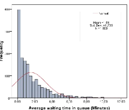
In Figure 3 is depicted a histogram of non-normal distribution of 1500 simulation replications together with mean=1.54 minutes, s=1.735, and normal distributed curve. Figure 4 indicates the non-normal by graphically comparing observed values to expected normal values.
Figure 3 Data distribution (N=1500)
Figure 4 Normality test (N=1500)
We also conducted Levene’s test for homogeneity of variances (see Table 4).
Results from tests showed us that the obtained data from the simulations is non- normal, and the variances are different. Subsequently, we did a quick research and we found that the simulation studies, applying a variety of non-normal distributions, show that the false positive rate is not affected very much by this violation of the assumption, as in reference [14-16]. This is because a large number of random samples from a population is approximately normally distributed even when the population is not normal. However, we decided to perform a non-parametric Kruskal-Wallis test, which substitutes for the one-way ANOVA. This non-parametric test does not assume that the data fit the normal distribution. It does assume that the data obtained from three simulation tools have the same distribution as each other.
Table 4
Levene’s test for homogeneity of variances (α=0.05)
Average waiting time in queue (Minutes) Levene Statistic df1 df2 p
Based on Mean 56.536 2 1497 <0.001
Based on Median 33.045 2 1497 <0.001
Based on Median and with adjusted df 33.045 2 1128.582 <0.001
Based on trimmed mean 46.539 2 1497 <0.001
Here we want to test a hypothesis that the results from all three simulation tools are equal. We state our hypothesis as:
H0:There is no difference between the three simulation tools (μArena=μSimul8= μWitness).
H1:At least one of the simulation tools gives different results due to generator number dissimilarity (not all μ’s are equal).
The results are summarized and presented in Tables 5 and 6. At significance level α=0.05, the final results show that there is significant difference between these outputs with respect to the average waiting time in queue. This seems to indicate that our preliminary expectations were not correct. According to our results, we do reject the null hypothesis. Another way to state this is: The difference between the three scenarios is statistically significant in this case.
Table 5
Summary of ranked data in each condition with Kruskal-Wallis test (α=0.05)
Simulation tool N Mean Rank Average waiting time in queue (Minutes) Arena 500 693.14
Simul8 500 715.81
Witness 500 842.55
Total 1500
Test statistic Chi-Square 34.754
df 2
p-value <0.001
The Kruskal-Wallis test indicates a significant effect of a group so we rejected hypothesis H0 and we applied a post-hoc test to determine which of the simulation tools is different. The Mann-Whitney test with Bonferroni correction compared all groups to each other. We compared Arena versus Simul8, Arena versus Witness, and Simul8versus Witness to identify the significance of the Kruskal-Wallis nonparametric test (see Table 6). We can conclude there is difference between Arena and Witness, and Simul8 and Witness.
Table 6
Test statistics for the Mann-Whitney test with Bonferroni correction (α=0.0167) Contrast Average waiting time in queue (Minutes)
Mann-Whitney U Wilcoxon W z p-value
Arena vs. Simul8 120960.000 246210.000 -0.888 0.375
Arena vs. Witness 100360.500 225610.500 -5.410 <0.001 Simul8 vs. Witness 103614.000 228864.000 -4.694 <0.001 Arena (Mdn=0.85) did not seem to differ in average waiting time in queue from Simul8 (Mdn=0.95), (U=120960, p=0.375, r=-0.03). The first comparison represents a very small effect because the effect size is close to zero. We can conclude that the effect on average waiting time in queue of Arena compared to Simul8 was negligible. On the other hand, Witness (Mdn=1.26) was significantly different from Arena (U=100360.5, p<0.001, r=-0.17) and Simul8 (U=103614,
p<0.001, r=-0.15). Because there was no significant difference between Arena and Simul8, we can assume that the random number generators of both simulation tools give the same random numbers. The small effect of Witness could lie in the equation (formula) for calculating the average performance indicators, which is different from Arena and Simul8. The average indicator in Witness counts all parts in the queue (or system) even when they are still in the queue (or in machine) at the end of the simulation. Arena and Simul8 determine the average waiting time indicators based on the parts that leave the queue (or system) at the end of the simulation run. Thus we can state that Witness determines the average performance indicator from an arrivals point of view, and Arena and Simul8 determine their average performance indicators from a departures point of view.
In this section, we investigated the congruence of the three different simulation software products based on their performance indicator, namely on the average waiting time in queue. We also identify the source of diversity between Witness and the other two simulation tools.
Conclusions
A simulation study was undertaken to investigate the effect of random number generators on performance indicators. The simulation study was applied to the M/G/1 manufacturing queuing model. The average waiting time in queue was used as the performance measure to explore the possible diversity between among the selected simulation tools.
After several simulation runs, we used the Kruskal-Wallis test, which revealed a significant effect of a group on value (H(3)=34.75, p<0.0001). A post-hoc test using the Mann-Whitney test was used to follow up the findings. The Bonferroni correction was also applied, and therefore all effects are reported at a 0.0167 level of significance. It appeared that the average waiting time in queue for Arena compared to Simul8 was no different (U=120960, r=-0.03). However, when Witness’s performance indicator was compared to Arena and Simul8, average waiting times were significantly different with small effect size.
The distinction between Arena and Witness, and Simul8 and Witness, lies in the addition of a formula that counts the average waiting time in the queue. Non- significance between Arena and Simul8 is due to the fact that they use a similar random number generator. Our findings on the three simulation tools also indicate that although they use a slightly different random generator, their results should be directed towards the same output. The size of the gains is significantly influenced by the formula for average waiting time.
Thus far, the analysis indicates that Witness has significantly different average waiting time than Arena and Simul8. This is due to the different equation formulae used in those simulation tools. The Witness simulation software includes in average waiting time also for parts (or entity) that remained in queue after terminating a simulation run (which seems to be more practical in manufacturing
planning and scheduling). Both Arena and Simul8 simulation software only count dispatched parts. This finding is also important from a practical perspective, because not knowing the behavior of performance indicators can lead to the wrong conclusion. This may occur by extending manufacturing lead time and increasing the cost of storing WIP, which was not considered in the beginning. This paper may be helpful for managers in selecting the appropriate simulation tool.
We hope that use of a simulation as presented will offer useful preliminary results for studying the throughput of a manufacturing system under various experimental conditions. We also proposed to add new criterion into evaluation framework of simulation software. This criterion is concerned with the type of the formula for average performance indicators (measures). Future research could address an approach to more difficult models, including the mean time between failures (MTBF) and the mean time to repair (MTTR).
References
[1] Shannon, R. E. (1998) Introduction to the Art and Science of Simulation.
IEEE, USA
[2] Murphy, C. A., Perera T. (2002) The Definition of Simulation and Its Role within an Aerospace Company. Simul Practice and Theory 9, 273-291 [3] Hlupic, V., Irani, Z., Paul, R. J. (1999) Evaluation Framework for
Simulation Software. International Journal of Advanced Manufacturing Technology 15, 366-382
[4] Sadiku, M. N. O., Ilyas, M. (1991) Simulation of Local Area Networks, CRC Press
[5] L'Ecuyer, P., Simard, R., Chen, E. J., Kelton, W. D. (2002) An Object- Oriented Random-Number Package with Many Long Streams and Substreams. Operational Research 50, 1073-1075
[6] Pusatli, O. T., Sanjay, M. (2011) Software Measurement Activities in Small and Medium Enterprises: an Empirical Assessment. Acta Polytechnica Hungarica 8(5), 21-42
[7] Gentle, E. J. (2003) Random Number Generation and Monte Carlo Methods. Springer, New York
[8] McHaney, R. (1991) Computer Simulation: A Practical Perspective.
Academic Press
[9] Fishman, G. S. (1990) Multiplicative Congruential Random Number Generators with Modulus 2beta: An Exhaustive Analysis for Beta = 32 and a Partial Analysis for Beta = 48. Mathematics of Computation 54, 331-344 [10] Sanjay, M. (2011) Evaluation Criteria for Object-oriented Metrics. Acta
Polytechnica Hungarica 8(5), 109-136
[11] Kelton, W. D., Sadowski, P. R., Sturock, T. D. (2007) Simulation with Arena. McGraw-Hill, New York
[12] Hauge, J. W., Paige, K. N. (2002) Learning SIMUL8: The Complete Guide. Plain Vu Publishers, Bethlingham
[13] Lanner Group (2000) WITNESS 2000 User Manual. Lanner Group, Oaks, UK
[14] Glass, G. V., Peckham, P. D., Sanders, J. R. (1972) Consequences of Failure to Meet Assumptions Underlying Fixed Effects Analyses of Variance and Covariance. Review of Educational Research 42, 237-288 [15] Harwell, M. R., Rubinstein, E. N., Hayes, W. S., Olds, C. C. (1992)
Summarizing Monte Carlo Results in Methodological Research: the One- and Two-Factor Fixed Effects ANOVA cases. Joutrnal of Educational Statistics 17, 315-339
[16] Lix, L. M., Keselman, J. C., Keselman, H. J. (1996) Consequences of Assumption Violations Revisited: A Quantitative Review of Alternatives to the One-Way Analysis of Variance F test. Review of Educational Research 66, 579-619