GÁBORKOHLRUSZ∗1 ANDDÉNESFODOR1
1Research Institute of Automotive Mechatronics and Automation, University of Pannonia, Egyetem u. 10, Veszprém, 8200, HUNGARY
Abstract - Since the energy consumption of electric drivetrains can be optimized in an automatically controlled system, the driving ranges and efficiency of driverless electric cars can be enhanced. The analysis of a model of the electric power conversion system provides the opportunity to consider different driving circumstances, moreover, it is possible to evaluate the performance of a power conversion system when the vehicle is driven along different routes. The results provide detailed information on the transient operation of all the power modules as well as their components, and on the overall performance of the power conversion system. In this study, a permanent-magnet synchronous machine (PMSM) acts as the traction motor in the autonomously driven electric car. Besides the PMSM, the power electronics and battery are also modeled in an OrCAD PSpice circuit-simulation environment that serves as a model of an electric power conversion system for the simulation and testing of a battery management system algorithm. The battery management system and control algorithm are modeled in Simulink and can be tested together with the PSpice-modeled circuits utilizing an interconnected simulation environment. The input of the power conversion system model was a driving scenario that included uphill and downhill sections. The performance of the implemented battery management system algorithm was analyzed and evaluated.
Keywords: electric power conversion system, autonomous vehicle, battery management, intercon- nected simulation
1. Introduction
A driverless car is an automated system where the driv- ing task is a self-acting function. As a result, it is possi- ble to optimize the energy efficiency of the car in order to increase its driving range and reduce its energy con- sumption. The optimal operation can be achieved by ap- plying well-designed control algorithms and battery man- agement functions.
The electric power conversion system of an au- tonomous vehicle is a very complex system, especially when the electronic control unit is also considered to be part of the system. During the test procedure of such a complexly controlled electric power conversion system, several unforeseen or unexpected behaviors can occur which may lead to damage. In order to avoid damage, it is essential to identify unexpected system behaviors as early as possible.
In the early phase of development, the testing and design of these systems should be performed simulta- neously to take advantage of the interconnected simu- lation environment. A mixed-signal simulation environ- ment supports the analysis of controlled electric power conversion systems where digital and analogue domains
∗Correspondence:kohlrusz.gabor@mk.uni-pannon.hu
can be connected and run simultaneously [1]. Simulations can be performed by taking into account practical aspects that introduce cycle times and delays into the model. In such a realistic simulation environment, the reliable de- sign of a battery management system can be achieved.
2. Electric Power Conversion System Model
A system model, including a model of the electronic con- trol unit, is a prerequisite to the simulation. The electric part of the system can be accurately modelled in a cir- cuit design environment, while the digital environment and control algorithm should be implemented in an en- vironment that is capable of running numerical computa- tions.
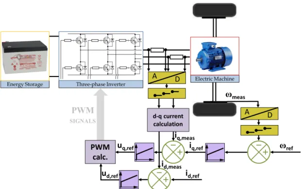
The electronic components were modeled in OrCAD PSpice environment while the control algorithm was re- alized in MATLAB-based Simulink. The electric parts of the modeled power conversion system can be seen in Fig. 1. The system consists of a Nickel Manganese Cobalt Oxide (NMC)-type Li-ion battery, a three-phase inverter and a permanent-magnet synchronous machine as the traction motor. The modeled system is a low-power counterpart of a vehicle power conversion system assum-
Figure 1:Structure of the Modeled Power Conversion System
ing that the system behavior is independent of the power rating.
2.1 Modeling of Energy Storage
The energy storage element of the modeled power con- version system is a Li-ion battery. The modeled battery cell consists of 4 individual NMC-type Sony VTC4A 2100 mAh battery cells connected in series. As Fig.2 shows, the model of the battery contains a State-of- Charge (SoC)-dependent voltage source and three passive components.
The model of the battery cell was developed and val- idated by using measurement data. A fully charged Sony VTC4A 2100 mAh battery cell was discharged slowly by setting the discharge current to a C/10 value until its volt- age reached the recommended minimum voltage level.
The time, battery voltage and discharge current were recorded and the SoC values were determined by time- integration of the current. Using the voltage and SoC time series, theU(SoC) function of the battery cell could be obtained by curve fitting. The best fit was achieved by
U = 0.227 log10
0.1
SoC + 3.35·10−5
+ 0.535 SoC3+ 3.8926 (1) The fitted curve and the measured voltages are shown to- gether inFig. 3as a function of the SoC.
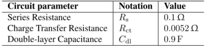
In order to complete the battery model, it is also nec- essary to obtain the electrical parameters of the battery cell. The values of the passive components were provided by measurements which put the transient behavior of the battery cell into focus. InTable 1, the values of all three parameters can be seen.
Figure 2:Equivalent Circuit Model of the Battery
Figure 3:Approximation of the Voltage Response of the Battery
2.2 Modeling of the Three-phase Inverter
The energy conversion between the electric motor and the battery was provided by a three-phase full-bridge inverter with 2 Metal–Oxide–Semiconductor Field-Effect Tran- sistor (MOSFET) semiconductors in each leg. The drive circuit was connected through a gate resistor to avoid an inrush current at the gate of the mosfets. The pulse-width modulated (PWM) gate-source voltages were provided by the digital controller which was implemented in the MATLAB-based Simulink environment.A schematic diagram of the inverter can be seen in Fig. 4. As the figure shows, a shunt resistor was added to each phase wire for current sensing.
2.3 Modeling of the Three-phase PMSM
In the modeled system, the traction motor was a permanent-magnet synchronous motor. The implemented model is valid for constructions with surface-mounted magnets on the rotor and distributed winding in the wye- wound stator.The electrical model was created by determining the voltages across the stator windings which consisted of
Table 1:Equivalent Circuit Model Parameters of the Bat- tery
Circuit parameter Notation Value
Series Resistance Rs 0.1Ω
Charge Transfer Resistance Rct 0.0052Ω Double-layer Capacitance Cdl 0.9 F
Figure 4:Three-phase Full-bridge Inverter
the resistive drop, the voltage across the inductor and the back electromotive force (back EMF). In the OrCAD en- vironment, it was quite easy to create the electric part of the motor model due to the fact that the voltage across the inductor in each phase could be represented by defining time-dependent self- and mutual inductances as passive components of the circuit, while their analytical model- ing would have been complicated.
The simulation of the motor requires the implementa- tion of the mechanical submodel as well. Papers dealing with the model of the three-phase PMSM also included the electromagnetic torque [2,3], however, it was chal- lenging to determine the expanded form of an expres- sion which could be easily implemented in an OrCAD environment. InRef.[4], a suitable form is presented for implementation in an OrCAD environment, hence this model was used in this work to obtain the mechanical model.
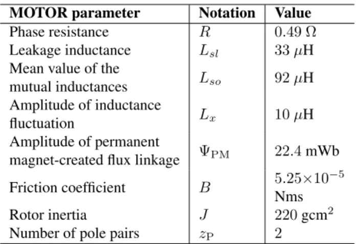
In the simulation, a MAXON EC-4pole 252463 type motor was considered. The parameters of the motor can be seen inTable 2.
3. Modeling of Electronic Control Unit
The Electronic Control Unit was modeled in a MATLAB- based Simulink environment which is suitable for quick algorithm and was equipped with an interface to OrCAD PSpice circuit simulation software.A realistic electronic control unit could be modeled using a trigger-activated Simulink function which run the control algorithm when a trigger signal is received.
The trigger signals were generated to fit the operating frequency of the digitally controlled discrete-time sys- tem. This solution ensured that the control algorithm only ran once during each sampling period, consequently, the Pulse Width Modulation (PWM) signals of each MOS- FET were generated only once during each sampling pe- riod. This solution is able to accurately simulate the op- eration of a microcontroller or even an electronic control unit.
The discrete-time control algorithm was implemented in the trigger-activated block. The structure of the algo- rithm can vary depending on how the difference equation is determined.
Amplitude of permanent
magnet-created flux linkage ΨPM 22.4mWb
Friction coefficient B 5.25×10⁻⁵
Nms
Rotor inertia J 220gcm2
Number of pole pairs zP 2
3.1 Discrete-Time Control Algorithm
The frequently used Proportional Integral (PI) algorithm was implemented to control the power conversion sys- tem. The structure of the control system is shown in Fig. 5. As the figure shows, a speed-cascaded torque con- trol loop and a magnetic field control loop were cre- ated. This strategy is the widespread field-oriented con- trol scheme of three-phase alternating current (AC) mo- tors.
In the case of a PI controller, the only dynamic com- ponent of the controller is the integrator since the pro- portional component simply multiplies the error signal.
Consequently, the proportional component can be imple- mented in the same form as in a continuous-time algo- rithm, however, the discrete-time form of the integrator has to be determined by using a Z-transform. The trans- formation can be conducted using different formulae to approximate the continuous-time system.
An easy way to determine the discrete-time form of the integrator is to use the backward Euler method. Using this method, the value of the integral at timejis
Yj =Yj−1+ejT TI (2) whereYjdenotes the result of the integral at timej,Yj−1
represents the result of the integral at timej−1,ejstands for the error signal at timej,T is the sampling time and TIdenotes the integral gain.
A drawback of this method is that a continuous-time system could be unstable in its discrete-time form using the backward Euler method [5].
The bilinear transform (also known as Tustin’s method) could be a more reasonable technique to obtain the discrete-time representation of a system since it pre- serves stability. The value of an integral at timejis de- termined by this method as follows:
Yj= Yj−1+ ej+ej−1 T TI
2 (3)
whereYjdenotes the result of the integral at timej,Yj−1 stands for the result of the integral at timej−1,ejrep- resents the error signal at timej,ej−1is the error signal
Figure 5:Vector-Controlled Power Conversion System of an Electric Vehicle
at timej−1,Tdenotes the sampling time andTIstands for the integral gain.
The realization of a controller that applies the back- ward Euler method is easier and this form generally pro- vides a stable operation, thus in the implemented model of a controller, the integrator was approximated byEq. 2.
3.2 Design of the Controller Parameters
The implemented controllers were PI controllers in paral- lel form, that is the integral and proportional terms were independent of each other.One of the simplest controller design procedures is the pole-zero cancellation but this method provides a fre- quency bandwidth for the controller that is identical with that of the controlled system resulting in poor perfor- mance occasionally. This problem is particularly severe when a system with a large time constant is controlled by a slow integrator with the same time constant as the system [6].
A better controller performance can be achieved by another analytical tuning method where the closed-loop poles are chosen to obtain an arbitrarily determined closed-loop Transfer function. The closed-loop is shaped by utilizing some predefined parameters such as the de- sired damping factor and bandwidth of frequencies.
The parameters of the PI controller can be computed as
Kc= 2ξω0τ−1
K (4)
whereKcdenotes the proportional gain of the controller, ω0stands for the natural frequency of the desired closed- loop system,ξrepresents the desired damping factor of
the second-order closed-loop system,τ is the time con- stant of the controlled first-order subsystem, andK de- notes the gain of the controlled first-order subsystem.
The value of the integral gain is determined as TI= ω02τ
K (5)
where ω0 denotes the natural frequency of the desired closed-loop system,τ stands for the time constant of the controlled first-order subsystem, and K represents the gain of the controlled first-order subsystem.
The damping ratio was chosen to ensure an overshoot of approximately 1%, therefore, for the computations, ξ = 0.85was applied. The desired natural frequency of the closed-loop system(ω0)was obtained by determin- ing the desired settling time of the controlled variable by considering a desired error band:
ω0=−lnp ξtb
(6) wherepdenotes the difference between the reference sig- nal and the value of the controlled variable as a percent- age of the reference value,ξstands for the desired damp- ing factor of the second-order closed-loop system, andtb
represents the period of time until the controlled variable is expected to reach the desired error band [7–9].
3.3 Implementation of the Smith predictor
When a discrete-time unit controls a system, a time delay is always present. During each time period, some mea- surements serve as the basis of control signal generation.controller output to be obtained. Based on the difference equation, the measurement signal was compensated by predicting the measurement value of the following time period:
1. At timeT1, measurement signaluˆ1is considered for the computation of controller outputy2 which will only take effect at timeT2.
2. Fromy2, it is possible to compute the predicted mea- surement valueuˆ2that can be used to obtainuˆ1−uˆ0
3. uˆ1=u1+ (ˆu1−uˆ0)is the corrected measurement signal, which is used to computey2 as has already been stated in Step 1:
whereu1 denotes the measured value of the controlled variable at timeT1 modified by the correction term, y2
stands for the controller output at timeT2,uˆ2represents the predicted value of the measurement at timeT2, anduˆ1
anduˆ1are the computed values of the controlled variable at timesT1andT0, respectively.
In Step 2, the difference equation of the controlled subsystem is used for the computation of the predicted
ˆ
u2 at timeT2. In the case of the current controllers, the prediction algorithm is
ˆ
ı2= (T2−T1)R L
U2
R −ˆı1
+ ˆı1 (7) where the currentˆı2 is the predicted value of the mea- surement signal at timeT2, which was the basis of the calculation of the correction termˆı1−ˆı0. The measured currenti1could be corrected as
ˆı1=i1+ (ˆı1−ˆı0). (8) The predictor was the same in both theid andiqcurrent controllers, only the parameters were different asLdwas substituted forEq. 7in case of theidcontrol loop andLq
was substituted forEq. 7in case of theiq control loop.
The Smith predictor in the cascade control loop requires the difference equation of the angular velocity as a func- tion of the currentiq:
ˆ
ω2= (T2−T1)1.5zPΨPMiq,1−Bωˆ1−MT
J + ˆω1 (9) The measured speedω1could also be corrected BY cal- culating the valuesωˆ1andωˆ0fromωˆ2:
ˆ
ω1=ω1+ (ˆω1−ωˆ0) (10)
Figure 6:Testing of theidandiqcurrent controllers
4. Testing of the Controlled Power Conver- sion System Model
The testing was performed with an operating frequency of 25 kHz in the control loop. The current controllers were designed to provide a settling time oftb = 2 ms withp = 0.02that equated to an error of2%which re- sulted in the desired frequency bandwidth ofω0 = 2301 rad/s. By taking into consideration the frequency band- width, the calculated controller parameters were
Kc,id= 0.12 (11) TI,id= 824 (12) for thed-axis current controller and
Kc,iq= 0.238 (13) TI,iq = 985 (14) for theq-axis current controller.
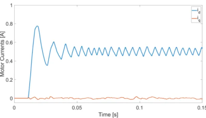
The testing of the controllers was performed without the implementation of the cascaded speed control loop. A reference current was set up for both current loops,dand q. The results can be seen inFigs. 6and7.
It is shown inFig. 6that the currentid overshot the reference value of0.5 Aand started to oscillate around the setpoint with an amplitude of50 mA, which is10%
of the reference value. The currentiq tracked its setpoint of0 Awith an inappreciable error. The results show that the integral gain of the currentid should be decreased, therefore, the controllers were tested with redesignedid
Figure 7:Results of the redesigned current controllers
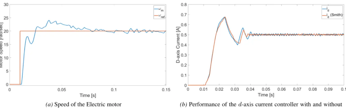
(a)Speed of the Electric motor (b)Performance of thed-axis current controller with and without the Smith predictor
Figure 8:Simulation results of the controlled system using the Smith predictor in the current controllers
controller while theiq controller parameters remain un- changed.
Kc,id= 0.12 (15) TI,id= 275 (16) for the current controllerd.
In Fig. 7, the results for the d-axis controller test- ing are presented. The performance of the redesignedd- axis current controllerid was enhanced. The controlled variable reached the setpoint and stabilized after approx- imately2 ms.
The angular velocityωwas controlled by a cascaded PI controller in theq-axis current loop. The controller pa- rameters were obtained by determining the desired fre- quency bandwidth which provided a settling time oftb= 0.05 sandp= 0.05, which equated to an error of5%:
Kc,ω= 0.038 (17)
TI,ω = 1.627 (18)
Fig. 8a shows the controlled motor-speed signal which has a reference value of20 rad/s. It can be seen that the speed signal overshot slightly and stabilized after0.065 s which was acceptable since the designed settling time was defined astb= 0.05 s.
4.1 Testing of the Smith predictor
The predictor was only implemented for the current con- trollers since the speed tracking performance of the sys- tem was satisfactory without the application of a predic- tor. The implemented predictor was tested under the same conditions as the current controllers, that is the current references id andiq were set at 0.5 Aand0 A, respec- tively.Fig. 8bshows the controller performance with and without the Smith predictor.
InFig. 8b, it can be seen that the controller performed better when the Smith predictor modified the error in the input signal of the controller by correcting the measured current signal. The controlled currentidstabilized faster and in a steady state it could be observed that the PWM- related high-frequency oscillation of the current occurred
with a reduced amplitude compared to when the Smith predictor was not applied. The behavior of the current signaliq did not change significantly since its reference value was set at0 Aand no dynamic changes in the ref- erence signal needed to be handled.
5. Battery Management System Design
The controlled power conversion system was validated by tests. The created model of the complex system is suit- able for simulations that are intended to analyze the op- eration of the system. By analyzing the operation of the power conversion system, the design aspects of a battery management system can be summarized. Simulation of the power conversion system can be a suitable procedure to validate the operation of the designed battery manage- ment system under realistic conditions.5.1 Implementation of a Battery Management System
When a battery management strategy is implemented, it influences both the hardware and software components of the supervised system. Battery management solutions ac- tuate in order to ensure efficient system operation as well as keep the system safe. If the management algorithm is used to ensure the system operates safely, all the avoided situations should be summarized during the design phase.
Moreover, for each undesirable situation, a hardware so- lution has to be designed, which can be activated when necessary.
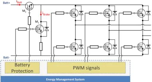
In this study, a battery overcharge protection system was analyzed as a battery management system. For this purpose, the power electronics had to be extended by ad- ditional power switches that were capable of changing operation mode when overcharging occurred (seeFig. 9).
The implementation of the battery management system also included augmentation of the software.
In Fig. 9, a power semiconductor (M1) can be seen that ensures an alternative path for the current when the battery cannot be charged. In this case, the recuperated energy is dissipated into a resistor. When switch M1 is
Figure 9:The analyzed battery management system
turned on, another switch (M2) becomes responsible for decoupling the battery, otherwise the battery would be discharged through the resistor. In certain situations, gen- eration of the PWM signal is also affected by the battery management algorithm. In this case, the PWM signals are generated in the same way whether the battery protection circuit operates or not.
5.2 Simulation of a Driving Cycle of a Vehicle
The simulation of a driving cycle of a vehicle provides the opportunity to observe the efficiency of the battery management strategy of the power conversion system and its interactions with the components of the system.The results serve as a basis for implementing different battery management strategies or modifying the imple- mented one.
A driving cycle can be simulated by defining differ- ent load torques of the traction motor. When an uphill or downhill stretch of road should be represented, the motor is loaded with a positive or negative load torque, respec- tively. If the gradients of the uphill and downhill sections of road are unchanged, the load torque remains constant.
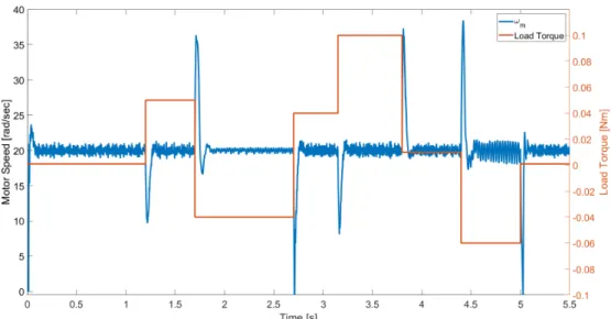
A simulation of5.5 sin duration was performed. The simulated driving cycle consisted of uphill, downhill and flat sections (seeFig. 10). In the picture, the load torques of the PMSM can also be seen below the corresponding sections of road. During the driving cycle, the speed of the vehicle was expected to be constant, hence the angular velocity was assumed to also be constant at20 rad/s. At the beginning of the simulation, it was assumed that the battery was fully charged.
The results of the simulation can be seen inFigs. 11 and12. InFig.11, the speed of the traction motor can be seen throughout the driving cycle. It can be observed that the changes in load torque influenced the speed of the motor, however, the controller promptly compensated for the transient overshoots.
Figure 10:Simulated vehicle path and related load torques
The currents of the power conversion system are pre- sented inFig. 12. The braking current and the current of the battery are also shown in Fig. 9. InFig. 12, it can be noted that theq-axis current controller achieved pre- cise and fast reference tracking when the system was per- turbed by changes in load torque. If the reference current iq was negative, the energy was recuperated, that is the traction motor was in generator operation mode. Since the battery was fully charged, energy must have been dis- sipated into the braking resistor. In the simulation, two cases when the battery management SYSTEM activated the braking circuit can be seen in the figure afterT1 = 1.7 sandT2 = 4.4 s. When the current flowed through the resistor the battery current was zero due to decoupling performed by switchM2. In the figure, a current spike can be easily observed when the battery was connected to the circuit after reference currentiqbecame positive.
6. Conclusions
This paper presents models of the power conversion sys- tem of an autonomous electric vehicle as well as the electronic control unit. An interconnected simulation en- vironment enables an integrated model to be simulated.
This kind of simulation is useful for the comparative per- formance analysis of different control algorithms as well
Figure 11:Simulated motor speed during the driving cycle of a vehicle
Figure 12:The simulated currents of the power conversion system with BMS
as system level analysis of interactions between different system modules and components.
A power conversion system model is very complex and it is hard to predict interactions between components of the system following dynamic changes at system in- puts. Furthermore, the validation of the controllers is only plausible if the simulation model includes all relevant components of the system and all significant factors such as sampling of the measured data or time delays in the control loop. The simulation is very useful if the opera- tion of the hardware level system is the focus of observa- tions and analyses.
However, the simulation of the top-level management system of an autonomous electric vehicle is not feasible due to lengthy simulation times. In order to analyze the performance of different controllers, the simulation must be run with a sampling time of 2 µs or less, while the effectiveness of a higher-level management system can be measured after a few hours of driving. In cases when
the analysis of the efficiency of the management system takes into consideration the performance of the digital controller, it is essential to identify a modeling procedure which provides a model of the system that is suitable for long-time simulation.
Acknowledgements
The project has been supported by the European Union, co-financed by the European Social Fund. (EFOP- 3.6.2- 16-2017-00002).
REFERENCES
[1] Kohlrusz, G.; Csomós, B.; Enisz, K.; Fodor, D.: Elec- tric energy converter development and diagnostics in mixed-signal simulation environment,ACTA Imeko, 2018,7(1), 20–26DOI: 10.21014/acta_imeko.v7i1.512
[2] Hang, J.; Zhang, J.; Cheng, M.; Huang, J.: On- line Interturn Fault Diagnosis of Permanent Magnet
Implementation of a Realistic Three-Phase PMSM Model for Diagnostic Purposes, San Diego, CA, USA, 2019, 372–376DOI: 10.1109/IEMDC.2019.8785371
[5] LeVeque, R. J.: Finite Difference Methods for Or- dinary and Partial Differential Equations: Steady- State and Time-Dependent Problems (Society for In- dustrial and Applied Mathematics, Philadelphia, PA,
[8] Katsuhiko, O.: Modern Control Engineering, (5th Edition) (Pearson), 2009ISBN: 0136156738
[9] Guzmán, J. L.; Moreno, J. C.; Berenguel, M.;
Moscoso, J.: Inverse pole placement method for PI control in the tracking problem, in IFAC-PapersOnLine, 51(4), 406–411 DOI:
10.1016/j.ifacol.2018.06.128