Evaluation and Improvement of Parallel Discrete Event Simulation Performance Predictions: A Rough-Set-based Approach

Evaluation and Improvement of Parallel Discrete Event Simulation Performance Predictions: A Rough-Set-based Approach

László Muka, István Derka

Department of Telecommunications, Széchenyi István University Egyetem tér 1, H-9026 Győr, Hungary; muka@sze.hu, steve@sze.hu

Abstract: Simulation performance prediction methods make possible the realization of performance improvement potentials of Parallel Discrete Event Simulation (PDES) methods, important in the analysis of complex systems and large-scale networks. Currently, high performance execution environments (emerging clusters and computing clouds) advance the development of quality/cost analysis capabilities of performance prediction methods. In this paper, for the evaluation and management of prediction correctness/cost, the efficacy, efficiency and effectiveness coefficients and improvement operations are defined for predictions. The performance coefficients and improvement operations are embedded in the rough-set-modeling and learning process and presented as an enhancement approach of the conventional Coupling Factor Method (CFM). A case study based on the CFM analysis of PDES of a closed queuing network model is presented. In the example, after rough-modeling and train-and-test analysis, the correctness/cost evaluation and effectiveness improvement operations are shown for series of predictions and the feedback connection to modeling refinement phase is demonstrated too.

Keywords: Parallel Discrete Event Simulation; simulation performance prediction;

quality/cost analysis; Systems Performance Criteria; Rough Set Theory; Coupling Factor Method

1 Introduction

Over the last few years, various research efforts have been made regarding Parallel Discrete Event Simulation (PDES) modeling and execution methods [1, 2, 3, 4], since parallel execution turned out to be an appropriate approach to meet high computing capacity requirements of Discrete Event Simulation (DES) analysis of complex systems and large-scale networks [5, 6].

In the present paper, PDES is defined as the execution of a single DES model on some high performance computing platform which can be clusters of homogeneous or heterogeneous computers and other emerging execution

Development of simulation models having high runtime performance features in a PDES execution environment is not an easy task even today, mainly because it is hard to tell the parallel execution features of a model, for example, possible resource capacity bottlenecks, in the development phase [7]. The simulation performance prediction of PDES execution can help to realize higher performance by providing preliminary knowledge about the behavior of the simulation model in the parallel execution environment [7, 8, 9, 10, 11]. The PDES performance prediction methods can support the performance increase throughout the whole modeling and simulation process including model development support, simulation setup and evaluation phases and taking into account different simulation framework specifics too [7].

Nowadays, emerging simulation operation forms, like on-line, real-time modeling and simulation and especially cloud computing with on-demand network access and pay-per-use feature and the developing simulation as a service (Simulation Software-as-a-Service) in public clouds [3, 21] put an increasing emphasis on quality/cost analysis capability of performance prediction methods.

The motivation of the authors to make the research presented in the paper was the lack of methods which can manage together the correctness and cost of performance prediction for a model in parallel simulation execution environment and which can also provide an easy feedback to the modeling and setup phases in the simulation.

The authors have developed the Enhanced Simulation Performance Prediction Method (ESPPM). ESPPM is enhancing the standard Coupling Factor Method (CFM) of PDES performance prediction [14] by a method of improvement allowing handle together correctness and cost in speedup predictions. The improvement approach based on Rough Set Theory (RST) [13] train-and-test analysis with embedded Systems Performance Criteria (SPC) [30] of efficacy (E1), efficiency (E2) and effectiveness (E3) for complex evaluation and quality/cost performance improvements steps.

In this work, the authors make the following key contributions:

 Definitions of performance improvement operations, based on definitions of cost measures and on definitions of performance coefficients of efficacy (E1), efficiency (E2) and effectiveness (E3) are described for single predictions and for series of predictions.

 A case study of the work of ESPPM is introduced using the example of a CFM PDES performance prediction of a Closed Queuing Network (CQN) model. In the analysis, the RST model of CFM modeling and its train-and-test examination is presented, the E1, E2 and E3 rule and attribute dropping operations are shown and the discussion of analysis results of performance predictions with feedback to the CFM and RST model-identification and refinement phase.

The rest of paper is organized as follows: Section 2 summarizes the related work, estimates the simulation performance prediction methods and relevant RST applications. Section 3 describes the components of the new method (RST, SPC and CFM). Section 4 introduces prediction performance improvement operations based on cost and prediction performance coefficients SPC-type definitions which are embedded into the process of train-and-test RST analysis. In Section 4, the process of ESPPM algorithm is described too. Section 5 introduces an example case study to demonstrate the use of the new method for the prediction analysis.

Section 6 discusses the results of analysis. Finally, the conclusions are presented.

2 Related Work

The related research is overviewed in following two points.

2.1 Simulation Performance Prediction Methods

The method introduced in [8] uses execution event-trace data of sequential and parallel, simulation runs, for creating the execution graph model and for the subsequent critical path analysis to predict parallel simulation performance. The method takes into account, in the prediction, the characteristics of the simulation hardware (with hardware parameters and mapping algorithms). The use of a wide variety of conservative and optimistic parallel simulation synchronization protocols is allowed by the method, which is an advantage. Unfortunately, the evaluation of prediction quality and the common evaluation with the cost of prediction are not treated in the method.

As an alternative to the conservative synchronization, the time driven version of the statistical synchronization method (SSM-T) with its loose synchronization [18, 19, 20] is a less well-known, but promising PDES synchronization method, that can be applied for the parallel simulation of certain types of systems such as communication networks. The increased performance can be predicted based on the trace of frequency of statistics exchange between segments. The frequency of statistics exchange can be used similarly to lookahead [15]. There is no performance model used in the method, thus, performance prediction requires time-consuming analysis of the simulation model operation.

The method described in [7], uses a hybrid approach to define the theoretical limit of the execution improvement for conservative synchronization protocol. In the trace-based part, the method analyses only a definite part of the sequence of events of the simulation model; while in an analytical modeling part, for the calculation of the lower bound on the runtime of the parallel simulation, a simplified scheduling problem model and the linear programming approach of is applied. An important advantage of this method is the definition of the

performance improvement limit for a model (or model version) but the method does not pay attention to the quality/cost analysis of predictions.

Paper [14] introduces the CFM (details are described in point 3.3), a simulation performance prediction approach, based on the coupling factor PDES performance model. The coupling factor helps to predict the parallelization potential of the simulation models and can be defined in sequential simulation model runs. The method is appropriate only for conservative null message-based algorithm. Unfortunately, CFM introduced in [14] does not predict the speedup value and does not support the quality/cost evaluation in predictions either.

2.2 Rough Set-based Performance Prediction

Paper [22] presents a rough set modeling and application runtime prediction method. The method is based on identifying and extracting properties defining runtime similarity of applications using available past data. The method does not include any consideration on prediction cost and on the improvement of prediction quality.

Paper [23] introduces a scheduling optimization approach for a dynamic remanufacturing situation with uncertain data. The proposed method is using linear programming and rough set evaluation and learning in an iterative process.

Monte Carlo simulation is also involved to improve consistency of data.

Unfortunately, complex evaluation, allowing quality/cost analysis in the learning process, is not included in the method.

3 Method Components

3.1 Rough Set Elements and the Rough Prediction Algorithm

The RST (Rough Set Theory) is a mathematical framework suitable for modeling and analysis of information systems with imprecise relations, with uncertain data [25, 26, 27, 28, 29].

A rough set information system with embedded knowledge consists of two sets:

the set of objects called the universe and the set of attributes.

More formally, 𝐼 = (𝑈, 𝐴, 𝑓, 𝑉) denotes an information system of RST, where set 𝑈 is the universe, 𝐴 is the set of attributes. Sets 𝑈 and 𝐴 are finite nonempty sets where (𝑈 = {𝑥1, 𝑥2, … , 𝑥_|𝑈|} and 𝐴 = {𝑎1, 𝑎2, … , 𝑎_|𝐴|}). The attributes define an information function 𝑓: 𝑈 → 𝑉 for 𝑈 where the set 𝑉 is the set of values of 𝐴 (𝑉 = 𝑉_𝑎1∪ 𝑉_𝑎2∪ … ∪ 𝑉_𝑎|𝐴|). The set 𝑉_𝑎𝑖– named also the domain of 𝑎_𝑖 – contains

the collection of values of 𝑎𝑖 and 𝑉𝑎_𝑖= {𝑣1_𝑎𝑖, 𝑣2_𝑎𝑖, … , 𝑣_|𝑉

𝑎𝑖| 𝑎𝑖

} where |𝑉𝑎_𝑖| is the size of the domain of 𝑎𝑖.

Discretization is the operation of mapping the primary values and ranges of all attributes to selected (possibly optimized) sets of discrete values: 𝑓_𝑉′: 𝑉^′→ 𝑉. The set 𝑉^′ stands for the values of 𝑎 before discretization.

The 𝐵-indiscernibility relation 𝐼𝑁𝐷(𝐵)for a set of attributes 𝐵 ⊆ 𝐴is defined in the following way:

𝐼𝑁𝐷(𝐵) = {(𝑥𝑖, 𝑥𝑗) ∈ 𝑈²|∀(𝑎 ∈ 𝐵)( 𝑎(𝑥𝑖) = 𝑎(𝑥𝑗))}.

If (𝑥𝑖, 𝑥𝑗) ∈ 𝐼𝑁𝐷(𝐵), then the objects 𝑥𝑖 and 𝑥𝑗 are indiscernible from each other in 𝐵 and the equivalence classes [𝑥]_{𝐼𝑁𝐷(𝐵)} of 𝐼𝑁𝐷(𝐵) are formed by the objects indiscernible in 𝐵.

Rough sets are defined by their lower approximation and upper approximation sets. The set 𝐵^∗(𝑋) and the set 𝐵∗(𝑋) is the 𝐵-lower and 𝐵-upper approximation of the set 𝑋 and defined as follows:

𝐵_∗(𝑋) = ⋃_𝑥∈𝑈{𝑥|[𝑥]_{𝐼𝑁𝐷(𝐵)}⊆ 𝑋} and 𝐵^∗(𝑋) = ⋃_𝑥∈𝑈{𝑥|[𝑥]_{𝐼𝑁𝐷(𝐵)}∩ 𝑋 ≠ ∅}.

The set 𝐵𝑁_𝐵(𝑋) defined by the equation 𝐵𝑁_𝐵(𝑋) = 𝐵^∗(𝑋) ∖ 𝐵_∗(𝑋) is the 𝐵- boundary region of 𝑋. If 𝑋 is a crisp set then, 𝑋 = 𝐵_∗(𝑋) thus 𝐵𝑁_𝐵(𝑋) = ∅ which means the boundary region is empty.

A reduct 𝑅_𝐵 is the minimal subset of attributes 𝐵 that allows the same classification of objects of 𝑈 as the set of attributes 𝐵. This feature of a reduct may be described by indiscernibility function as follows:

𝐼𝑁𝐷_{∀𝑥(𝑥∈𝑈)}(𝑅_𝐵) = 𝐼𝑁𝐷_{∀𝑥(𝑥∈𝑈)}(𝐵), 𝐵 ⊆ 𝐴.

In general, the information system may take the form of 𝐼 = (𝑈, 𝐴 = 𝐶 ∪ 𝐷, 𝑓, 𝑉) which is a decision information system (DIS). The set 𝐶 = {𝑐1 , 𝑐2 , … , 𝑐_|𝐶|} denotes the set of condition attributes and 𝐷 is the set of decision attributes 𝐷 = {𝑑₁ , 𝑑₂ , … , 𝑑_|𝐷|}. The information function 𝑓: 𝑈 → 𝑉 may be expressed by information functions 𝑓_𝐶: 𝐶 → 𝑉_𝐶 and 𝑓_𝐷: 𝐷 → 𝑉_𝐷, where 𝑉 = 𝑉_𝐶∪ 𝑉_𝐷 (𝑉_𝐶 = 𝑉_𝑐1∪ 𝑉𝑐₂∪ 𝑉𝑐₃∪, … ,∪ 𝑉𝑐_|𝐶| and 𝑉𝐷 = 𝑉𝑑₁∪ 𝑉𝑑₂∪ … ∪ 𝑉𝑑_|𝐷|) and

𝑉𝐶 = ⋃|𝐶| 𝑉𝑐_𝑖

𝑖=1 where 𝑉𝑐_𝑖={𝑣1_𝑐𝑖, 𝑣2_𝑐𝑖, … , 𝑣_|𝑉

𝑐𝑖| 𝑐𝑖

} and 𝑉𝐷 = ⋃|𝐷| 𝑉𝑑_𝑖

𝑖=1 . where 𝑉_𝑑𝑖={𝑣₁

𝑑𝑖, 𝑣₂

𝑑𝑖, … , 𝑣_|𝑉

𝑑𝑖| 𝑑𝑖

}.

In a decision table𝐼 = (𝑈, 𝐴 = 𝐶 ∪ {𝑑}, 𝑓, 𝑉) based on a DIS, 𝑑 denotes the distinguished decision attribute. Furthermore, a decision information system having the form of 𝐼 = (𝑈, 𝐶 ∪ 𝐷, 𝑓_𝑉′, 𝑓, 𝑉^′, 𝑉) denotes a DIS with discretization information functions 𝑓_𝑉𝐶^′: 𝑉𝐶′→ 𝑉𝐶and 𝑓_𝑉𝐷^′: 𝑉𝐷′→ 𝑉𝐷.

The classification may also be described by a set decision rules 𝑆 = {𝑠1, 𝑠2, … , 𝑠_|𝑆|} in the form of implication 𝑠𝑘 = (𝜑𝑘⇒ 𝜅𝑘), (𝑠_𝑘 ∈ 𝑆), where 𝜑𝑘 and 𝜅𝑘 are logical expressions of the condition and decision attributes respectively. The formulas 𝜑𝑘 and 𝜅𝑘 may also be quoted as LHS (Left Hand Side) and RHS (Right Hand Side) part of the rule. A decision rule 𝑠𝑘 may be evaluated by its 𝑀𝑎𝑡𝑐ℎ𝑈(𝑠𝑘) and 𝑆𝑢𝑝𝑝𝑈(𝑠𝑘) values, where 𝑀𝑎𝑡𝑐ℎ𝑈(𝑠𝑘) is the number of objects in 𝑈 the attribute values of which satisfy 𝜑_𝑘 (matching with the LHS part of 𝑠_𝑘), and 𝑆𝑢𝑝𝑝_𝑈(𝑠_𝑘) denotes the number of objects in decision table the attribute values of which satisfy both 𝜑_𝑘 and 𝜅_𝑘 (matching with both the LHS and RHS parts of 𝑠_𝑘).

Figure 1

The Traditional Rough Set Theory (TRST) analysis algorithm for performance prediction Figure 1 shows the process of the rough prediction algorithm. The essence of the algorithm is the random split of the universe into train and test partitions, generation a set of classification rules using the train partition and then generation classification predictions for the test partition using the generated rules.

3.2 Systems Performance Criteria

Efficacy (E1), efficiency (E2) and effectiveness (E3) are Systems Performance Criteria (SPC) [11, 30, 31]. E1, E2 and E3 coefficients are in a hierarchy-like relationship with each other. On the longer term, the performance of a system is checked by the effectiveness criterion, the efficacy criterion shows whether the performance is suitable at all, and the efficiency criterion characterizes the relation of the required output and the resources used to produce the output.

Generating the set of classification rules : Predicting classification of 𝑈_{𝑡𝑒𝑠𝑡} according to 𝑆_{𝑡𝑟𝑎𝑖𝑛}:

Decision Information System : Decision table (selecting a single decision attribute) :

Splitting the universe :

𝑓𝑝𝑟𝑒𝑑𝑖𝑐𝑡𝑖𝑜𝑛 : 𝑈_{𝑡𝑒𝑠𝑡}× 𝑆_{𝑡𝑟𝑎𝑖𝑛} → {𝑉_𝑑 , 𝑢𝑛𝑑𝑒𝑓𝑖𝑛𝑒𝑑}

𝑓_{𝑅𝑁𝐷𝑠𝑝𝑙𝑖𝑡}: 𝑈 → (𝑈_{𝑡𝑟𝑎𝑖𝑛}∪ 𝑈_{𝑡𝑒𝑠𝑡})

𝑓𝑟𝑢𝑙𝑒 𝑔𝑒𝑛𝑒𝑟𝑎𝑡𝑖𝑜𝑛: 𝑈_{𝑡𝑟𝑎𝑖𝑛}× 𝐺 → 𝑆_{𝑡𝑟𝑎𝑖𝑛} Selection the reduct and rule generation method 𝐺

𝐼= (𝑈, 𝐴 = 𝐶 ∪ {𝑑 }, 𝑓, 𝑉), 𝑑 ∈ 𝐷 𝐼= (𝑈, 𝐴 = 𝐶 ∪ {𝑑 }, 𝑓, 𝑉)

3.3 The Coupling Factor Method

Based on some theoretical considerations about the connectedness of PDES model segments, paper [14] describes a practical simulation performance prediction approach the Coupling Factor Method (CFM). The method – using results of sequential simulation runs – predicts the parallelization potential of simulation models with conservative null message-based synchronization algorithm. The CFM performance model can be described by the formula:

𝜆 = 𝐿 ∗ 𝐸 𝜏 ∗ 𝑃⁄

where 𝐿 is the lookahead value characterizing the simulation model [𝑠𝑖𝑚𝑠𝑒𝑐] [6], 𝐸 is the event density generated by the model [𝑒𝑣𝑒𝑛𝑡 𝑠𝑖𝑚𝑠𝑒𝑐⁄ ], 𝜏 is the latency of messages between logical processes (LPs) of the simulation model during the execution [𝑠𝑒𝑐], and 𝑃 is the event processing hardware performance [𝑒𝑣𝑒𝑛𝑡 𝑠𝑒𝑐⁄ ]. In this performance model, parameters 𝐿 and 𝐸characterize the simulation model itself, parameters 𝜏 and 𝑃 describe the execution environment.

The performance model involves only four parameters for the performance prediction calculations that can be measured in simple sequential simulation runs.

According to the method, the PDES speedup value cannot be predicted, but the high value of 𝜆 (𝜆value is a couple of time 100 or higher [15]) shows the good potential for simulation model parallelization. For a separate process, the 𝜆𝑁

parallelization potential of a process is only a part of the whole potential:

𝜆𝑁= 𝜆 𝑁⁄ 𝐿𝑃

where 𝑁𝐿𝑃 the number of LPs [15]. (The four parameters of CFM formulates requirement on the simulation model and on how the parallelization potential can be exploited.)

The method has been validated by a series of simulation investigations for homogeneous and heterogeneous clusters of computers [15, 16, 17]. Example applications for telecommunication systems and for cloud computing systems have been introduced too in [16] and [32].

4 The Prediction Performance Enhancement

4.1 Defining Prediction Performance Coefficients

In a TRST simulation performance analysis, in a decision table 𝐼 = (𝑈, 𝐴 = 𝐶 ∪ {𝑑}, 𝑓, 𝑉) the objects of the universe 𝑈 are computer simulation experiments. Set of attributes (𝐴) consists of independent (𝐶) and dependent {𝑑} variables that are taken into account in performance evaluation and in classification prediction.

The classification of experiments in 𝑈𝑡𝑒𝑠𝑡(𝑖) (𝑈 = 𝑈𝑡𝑟𝑎𝑖𝑛(𝑖) ∪ 𝑈𝑡𝑒𝑠𝑡(𝑖)) is predicted by 𝑓𝑝𝑟𝑒𝑑𝑖𝑐𝑡𝑖𝑜𝑛(𝑖): 𝑈_{𝑡𝑒𝑠𝑡(𝑖)}× 𝑆_{𝑡𝑟𝑎𝑖𝑛(𝑖)}→ {𝑉_𝑑 , 𝑢𝑛𝑑𝑒𝑓𝑖𝑛𝑒𝑑}, (𝑖 = 1,2, … , n), using the set of rules 𝑆𝑡𝑟𝑎𝑖𝑛(𝑖)= {𝑠1, 𝑠2, … , 𝑠_{|𝑆𝑡𝑟𝑎𝑖𝑛(𝑖)|}} , 𝑠𝑘 = 𝜑𝑘⇒ 𝜅𝑘 that are generated according to function 𝑓_{𝑡𝑟𝑎𝑖𝑛}: 𝑈_{𝑡𝑒𝑠𝑡}× 𝐺 → 𝑆_{𝑡𝑟𝑎𝑖𝑛} in TRST.

In the following the E1, E2 and E3 SPC will be defined in the form of prediction performance coefficients: efficacy (E1) to measure prediction correctness, efficiency (E2) to assess correctness-to-cost relationship and effectiveness (E3) to take into account E1 and E2 for series of predictions. To calculate cost relationships cost of experiments, attributes, rules and predictions will be defined using the consumed computation time.

For the improvement of prediction performance, attribute and rule dropping operations are defined.

Definition 1. Efficacy (E1) of a prediction 𝐸1𝑝𝑟𝑒𝑑𝑖𝑐𝑡𝑖𝑜𝑛 is calculated according to formula 𝐸1_{𝑝𝑟𝑒𝑑𝑖𝑐𝑡𝑖𝑜𝑛}=^{∑|𝑈𝑡𝑒𝑠𝑡|𝑙=1}_|𝑈 ^{𝑝(𝑥𝑙)}

𝑡𝑒𝑠𝑡|

where 𝑝(𝑥𝑙) (prediction correctness) is equal to 𝑝(𝑥𝑙) = {1, |〈𝑑(𝑥_𝑙)_{𝑝𝑟𝑒𝑑𝑖𝑐𝑡𝑒𝑑}〉 = 〈𝑑(𝑥_𝑙)_{𝑜𝑏𝑠𝑒𝑟𝑣𝑒𝑑}〉

0|𝑜𝑡ℎ𝑒𝑟𝑣𝑖𝑠𝑒 and where𝑑(𝑥𝑙)_{𝑝𝑟𝑒𝑑𝑖𝑐𝑡𝑒𝑑} is 𝑑(𝑥𝑙)_{𝑝𝑟𝑒𝑑𝑖𝑐𝑡𝑒𝑑}= {𝑣𝑑, 〈𝜅𝑘〉 = 𝑣𝑑, 𝑣𝑑∈ 𝑉𝑑|(𝑀𝑎𝑡𝑐ℎ𝑈_{𝑡𝑒𝑠𝑡}(𝑠𝑘) = 1

𝑢𝑛𝑑𝑒𝑓𝑖𝑛𝑒𝑑 |𝑜𝑡ℎ𝑒𝑟𝑣𝑖𝑠𝑒 and (𝑠𝑘 ∈ 𝑆𝑡𝑟𝑎𝑖𝑛), 〈𝑑(𝑠𝑘)𝑝𝑟𝑒𝑑𝑖𝑐𝑡𝑒𝑑〉 = 𝑣_𝑑(𝑥

𝑙,𝑠_𝑘).

The interval of 𝐸1 coefficient is 0 ≤ 𝐸1 ≤ 1. If 𝐸1𝑝𝑟𝑒𝑑𝑖𝑐𝑡𝑖𝑜𝑛≥ 𝐸1𝑙𝑖𝑚𝑖𝑡 is true then the prediction is efficacious. The 𝐸1𝑙𝑖𝑚𝑖𝑡 denotes the lower limit of efficacy and the inequality 𝐸1𝑙𝑖𝑚𝑖𝑡> 0.5 should be satisfied that is the efficacy of prediction is required to be better than random guess.

Definition 2. Cost of experiments, attributes, rules and predictions

For a decision table 𝐼 = (𝑈, 𝐴 = 𝐶 ∪ {𝑑}, 𝑓, 𝑉) supposing that a homogeneous cluster of computers with equal cores is examined and supposing that all the cores are continuously working during the execution time, the cost of a simulation experiment 𝑥𝑙(𝑥_𝑙∈ 𝑈) is defined as: 𝐾(𝑥𝑙) = 𝑁_{𝑐𝑜𝑟𝑒𝑠}∗ 𝑒𝑥𝑒𝑐𝑢𝑡𝑖𝑜𝑛 𝑡𝑖𝑚𝑒 [𝑠𝑒𝑐].

Cost of a rule 𝑠_𝑘 is calculated as 𝐾(𝑠_𝑘) = ∑^|𝑈|_𝑙=1𝐾(𝑥_𝑙|𝑆𝑢𝑝𝑝(𝑠_𝑘)) = 1) [𝑠𝑒𝑐].

Cost of a prediction 𝐾(𝑆𝑝𝑟𝑒𝑑𝑖𝑐𝑡𝑖𝑜𝑛) is defined as 𝐾(𝑆𝑡𝑟𝑎𝑖𝑛) = ∑^|𝑆_𝑘=1^{𝑡𝑟𝑎𝑖𝑛|}𝐾(𝑠𝑘)[𝑠𝑒𝑐], (𝑠𝑘 ∈ 𝑆𝑡𝑟𝑎𝑖𝑛).

Definition 3. Efficiency (E2) of a prediction 𝐸2𝑝𝑟𝑒𝑑𝑖𝑐𝑡𝑖𝑜𝑛= 𝐸1𝑝𝑟𝑒𝑑𝑖𝑐𝑡𝑖𝑜𝑛⁄𝐾𝑝𝑟𝑒𝑑𝑖𝑐𝑡𝑖𝑜𝑛 [_𝑠𝑒𝑐¹]

Definition 4. Effectiveness (E3) of a series of predictions 𝐸3𝑠𝑒𝑟𝑖𝑒𝑠= 𝐸3(𝑆𝑝𝑟𝑒𝑑𝑖𝑐𝑡𝑖𝑜𝑛) = 𝐸2𝑛|𝐸1𝑛 where

𝐸1_𝑛=_𝑛¹∑^𝑛_𝑖=1𝐸1_(𝑖) and 𝐸2_𝑛=¹_𝑛∑^𝑛_𝑖=1𝐸1_(𝑖)⁄¹_𝑛∑^𝑛_𝑖=1𝐾(𝑆_{𝑡𝑟𝑎𝑖𝑛(𝑖)}) [_𝑠𝑒𝑐¹]

and where 𝑖 denotes the 𝑖-th prediction and 𝑛 is the number of predictions in the series( 𝑛 ≥ 2). For 𝑛 = 1 𝐸3𝑠𝑒𝑟𝑖𝑒𝑠 is undefined and for 𝐸1𝑛< 𝐸𝑙𝑖𝑚𝑖𝑡 𝐸3𝑠𝑒𝑟𝑖𝑒𝑠 is not effective.

Definition 5. Rule and attribute dropping

Dropping of a rule 𝑠_𝑘 and dropping of an attribute 𝑐_𝑗 for the pair (𝑆_{𝑡𝑟𝑎𝑖𝑛}, 𝑈_{𝑡𝑒𝑠𝑡}) are the replacement operations 𝑆𝑡𝑟𝑎𝑖𝑛∶= 𝑆𝑡𝑟𝑎𝑖𝑛∖ {𝑠𝑘} and 𝐶 ∶= 𝐶 ∖ {𝑐_𝑗} respectively.

4.2 The Enhanced Simulation Performance Prediction Method

Figure 2 shows the process diagram of the Enhanced Simulation Performance Prediction Method (ESPPM).

The ESPPM process can be described as follows:

 The ESPPM input data are produced both in sequential (CFM parameter measurements) and parallel simulation model runs (PDES, CFM parameter measurements, runtime measurements for cost calculations are executed and other relevant (or possibly relevant) simulation modeling hardware and software environmental data are collected.

 The rough model is made for performance prediction (objects and attributes of DISs before and after discretization).

 The TRST train-and-test method is used in interactive manner for generation of predictions

 The E1, E2 and E3 coefficients (built in the TRST cycle) are used for evaluation and attribute and rule dropping operations are applied for improvement of correctness and cost of predictions.

 The method supports setting up feedback to identification and refinement phase of the simulation performance prediction models.

The method can be implemented by using the OMNet++ [12] and the Rosetta System [13] free software for DES modeling and RST examinations respectively.

Figure 2

The process of the Enhanced Simulation Performance Prediction Method (ESPPM)

5 Prediction Performance Analysis Case Study

5.1 Simulation Performance Evaluation Example

The example analysis of the CFM approach described in [15] investigates the simulation runs of a CQN model with various configurations in a homogeneous cluster execution environment with different number of processors.

In Figure 3, the number of tandem queues in the CQN model is 24 (𝑄1,…,24), the number of simple queues in a tandem queue is 50 (𝑞1,…,50). The switching between tandem queues is performed by switches (𝑠𝑤1,…,24) according to uniform probability distribution. The delay of switching between tandem queues (shown by 2D arrow shapes, in Figure 3) will model the lookahead (𝐿). The lookahead delay is the delay of a job before entering the next tandem queue and it is defined by the 𝐿 value.

TRST

Sequential simulation model run to generate prediction inputs Parallel simulation model run to generate validation data

𝐼 = (𝑈, 𝐶 ∪ 𝐷, 𝑓𝑉^′, 𝑓, 𝑉^′, 𝑉) 𝑓 𝑐𝑜𝑠𝑡: 𝑀(𝑠𝑖𝑚𝑢𝑙𝑎𝑡𝑖𝑜𝑛 𝑟𝑢𝑛 )→ 𝑀(𝑟𝑢𝑛𝑡𝑖𝑚𝑒 𝑐𝑜𝑠𝑡 )= {𝐾}

Efficacy (E1) evaluation, Attribute and rule dropping

experiments

Efficiency (E2) evaluation, Attribute and rule dropping

experiments

Effectiveness (E3) evaluation, Attribute and rule dropping

experiments Approximation space

condensing

Feedback to simulation models Feedback to RST models before

discretization

Prediction performance management Setting up decision

information systems and tables

Figure 3

CQN model for PDES performance simulation

The starting number of jobs in every simple queue is 2 jobs, thus the number of jobs in CQN is 2400 and this value remains constant. Jobs have exponential inter- arrival time and exponential service time distributions with FCFS service discipline. The expected value for both the arrival and service time distributions is 10𝑠𝑖𝑚𝑠𝑒𝑐. The delay on links between simple queues is 1𝑠𝑖𝑚𝑠𝑒𝑐.

The software environment of simulation runs includes: Linux (Debian) operating system, MPI, NFS, OMNet++ network simulator. The hardware environment of simulation runs is a homogeneous cluster of 12 two-core host PCs. The communication latency of messages – measured by the OpenMPI PingPong benchmark and used as 𝜏 value – over MPI between the host PCs of the cluster is 25𝜇𝑠𝑒𝑐.

To calculate coupling factor 𝜆 the values of𝐸 and 𝑃 variableswere measured in sequential simulation runs on one core of a host PC (𝑁𝑐𝑜𝑟𝑒𝑠=1) with 𝐿 =0.1, 1, 10, 100 and 1000 𝑠𝑖𝑚𝑠𝑒𝑐 of lookahead values. The result of sequential simulation runs is summarized in Table 1 [15].

Table1

Coupling factor determination by sequential simulations

The PDES experiments were executed using equal number of cores and LPs:

𝑁𝐿𝑃= 2, 4, 6, 8, 12 and 24 (𝑁𝑐𝑜𝑟𝑒𝑠= 𝑁𝐿𝑃). The relative speedup results measured in PDES executions are summarized in Table 2.

The simulated virtual time both for sequential and PDES runs was 864000𝑠𝑖𝑚𝑠𝑒𝑐.

The total number of execution runs for sequential simulation and for PDES were

q

Q

Q

...

...

q

q

q

Q

...

q

q

q

q

q

...

sw

sw

sw

L [simsec] 0.1 1 10 100 1000

Execution time [sec] 524.18 521.36 523.09 516.54 415.73 P [ev sec⁄ ] 263502 264868 263465 261132 247653 E [ev simsec⁄ ] 159.86 159.83 159.51 156.12 119.16 Coupling factor λ 2.43 24.14 242.17 2391.39 19246.76

Table 2

PDES relative speedup performance at different N_cores and L values

L [simsec] 0.1 1 10 100 1000

Ncores=2 0.43 0.78 0.85 0.99 0.99

N_cores=4 0.06 0.48 0.83 0.92 0.94

Ncores=6 0.03 0.28 0.76 0.91 0.94

N_cores=8 0.02 0.18 0.66 0.89 0.95

Ncores=12 0.01 0.09 0.48 0.86 0.94

Ncores=24 0.00 0.02 0.18 0.63 0.87

The speedup is defined as a proportion of the sequential and the PDES execution time of the simulation. The relative speedup is calculated as the proportion between the speedup values and the number cores used to achieve the speedup.

5.2 RST Modeling and Analysis

The RST model of simulation performance prediction is presented in the form of decision information systems and decision tables:

𝐼 = (𝑈, 𝐶 ∪ 𝐷, 𝑓_𝑉^′, 𝑓, 𝑉^′, 𝑉), 𝐼 = (𝑈, 𝐴 = 𝐶 ∪ 𝐷, 𝑓, 𝑉), 𝐼 = (𝑈, 𝐴 = 𝐶 ∪ {𝑑}, 𝑓, 𝑉, ), 𝑑 ∈ 𝐷.

An extended but relevant list of elements of 𝑈, 𝐶 and 𝐷 sets are described below.

The simulation experiments are the objects of the universe 𝑈 = {𝑥₁, 𝑥₂, 𝑥₃, … , 𝑥₃₀} where 𝑥_𝑖 denotes the object of the universe with index 𝑖.

An extended set of condition attributes may be defined as follows

𝐶 = { 𝑃, 𝐸, 𝐿(𝑐₀₄), 𝜆(𝑐₀₁), 𝜆_𝑁, 𝑁_𝐿𝑃, 𝑁_{𝑐𝑜𝑟𝑒𝑠}(𝑐₀₃), 𝜏, 𝑠𝑖𝑚𝑢𝑙𝑎𝑡𝑒𝑑 𝑣𝑖𝑟𝑡𝑢𝑎𝑙 𝑡𝑖𝑚𝑒, } ∪ {𝑐𝑜𝑛𝑠𝑒𝑟𝑣𝑎𝑡𝑖𝑣𝑒 𝑠𝑦𝑛𝑐ℎ𝑟𝑜𝑛𝑖𝑠𝑎𝑡𝑖𝑜𝑛 𝑝𝑟𝑜𝑡𝑜𝑐𝑜𝑙 𝑤𝑖𝑡ℎ 𝑛𝑢𝑙𝑙 𝑚𝑒𝑠𝑠𝑎𝑔𝑒 𝑎𝑙𝑔𝑜𝑟𝑖𝑡ℎ𝑚} ∪ { 𝑄, 𝑞, 𝑛𝑢𝑚𝑏𝑒𝑟 𝑜𝑓 𝑗𝑜𝑏𝑠 𝑖𝑛 𝐶𝑄𝑁, 𝑖𝑛𝑡𝑒𝑟 𝑎𝑟𝑟𝑖𝑣𝑎𝑙 𝑡𝑖𝑚𝑒,

𝑠𝑒𝑟𝑣𝑖𝑐𝑒 𝑡𝑖𝑚𝑒, 𝐹𝐶𝐹𝑆 𝑠𝑒𝑟𝑣𝑖𝑐𝑒 𝑑𝑖𝑠𝑐𝑖𝑝𝑙𝑖𝑛𝑒, 𝑠𝑤𝑖𝑡𝑐ℎ𝑖𝑛𝑔 𝑡𝑖𝑚𝑒 𝑏𝑒𝑡𝑤𝑒𝑒𝑛 𝑡𝑎𝑛𝑑𝑒𝑚𝑠, 𝑝𝑟𝑜𝑝𝑎𝑔𝑎𝑡𝑖𝑜𝑛 𝑑𝑒𝑙𝑎𝑦 𝑏𝑒𝑡𝑤𝑒𝑒𝑛 𝑠𝑖𝑚𝑝𝑙𝑒 𝑞𝑢𝑒𝑢𝑒𝑠 } ∪

{ 𝑂𝑀𝑁𝑒𝑡 + +, 𝑀𝑃𝐼, 𝐿𝑖𝑛𝑢𝑥 𝐷𝑒𝑏𝑖𝑎𝑛 }.

The set of decision attributes under consideration can be set as

𝐷 = {𝑟𝑒𝑙𝑎𝑡𝑖𝑣𝑒 𝑠𝑝𝑒𝑒𝑑𝑢𝑝(𝑑₀₁), 𝑠𝑝𝑒𝑒𝑑𝑢𝑝(𝑐₀₂, 𝑑₀₂), 𝑢𝑡𝑖𝑙𝑖𝑧𝑎𝑡𝑖𝑜𝑛 𝑜𝑓 𝑟𝑒𝑠𝑜𝑢𝑟𝑐𝑒𝑠}.

(The variables in brackets (for example, 𝑐₀₄) shows the variables selected for the analysis.)

5.2.1 Generating Predictions and Costs

For the prediction performance analysis the following decision table after discretization and appropriate coding is used:

𝐼 _𝑑01= (𝑈, 𝐴 = 𝐶 ∪ { 𝑑₀₁}, 𝑓, 𝑉), 𝑈 = {𝑥₁, 𝑥₂, … , 𝑥₃₀}, 𝐶 = {𝑐₀₁, 𝑐₀₂, 𝑐₀₃, 𝑐₀₄}, 𝑉𝑐₀₁= {𝑙, 𝑚, ℎ, 𝑠, 𝑒}, 𝑉𝑐₀₂= {𝑎, 𝑛}, 𝑉𝑐₀₃= {2,4,6,8,12,24},

𝑉𝑐₀₄= {𝑓(𝑣𝑐′₀₄= 0.1), 𝑔, ℎ, 𝑜, 𝑡(𝑣𝑐′₀₄= 1000)}, 𝑉𝑑₀₁= {𝐿(0 ≤ 𝑣_𝑑^′₀₁< 0.6), 𝐻}.

(For the later analysis, some values are shown before coding too (for example, 𝑣𝑐′₀₄= 0.1))

The examination is performed in a form of TRST train-and-test analysis. For the train-and-test examination, based on our previous results presented in [24], the Rosetta System [13] is used with G=Johnson’s RSES (Rough Set Exploration System) reduct and rule generation method and with the subsequent classification of objects. The algorithm of examination is as follows:

Input: 𝐼 _𝑑01, simulation runtime and configuration data, TRST configuration setup data: (𝑈 = 𝑈𝑡𝑟𝑎𝑖𝑛(𝑖)∪ 𝑈𝑡𝑒𝑠𝑡(𝑖)) ∧ ((𝑈𝑡𝑟𝑎𝑖𝑛(𝑖)∩ 𝑈𝑡𝑒𝑠𝑡(𝑖)) = ∅) ∧ (|𝑈𝑡𝑟𝑎𝑖𝑛(𝑖)| |𝑈|⁄ =

=¹⁵₃₀) ∧ ( 𝑅𝑁𝐷𝑠𝑒𝑒𝑑 = 𝑖) ∧ (𝐺 = 𝐽𝑜ℎ𝑛𝑠𝑜𝑛^′𝑠 𝑅𝑆𝐸𝑆)

Output: approximation of classification prediction data, and SPC evaluation begin

for i=1 to 8 for each prediction case do //prediction cases = 0, 3, 4,

compute TRST

//for the series of computation use the same (𝑈𝑡𝑟𝑎𝑖𝑛(𝑖), 𝑈𝑡𝑒𝑠𝑡(𝑖)) //pairs (𝑖 = 1,2, … ,8)

return classification prediction rules and classification prediction data, E1, E2 and E3 evaluation data

end

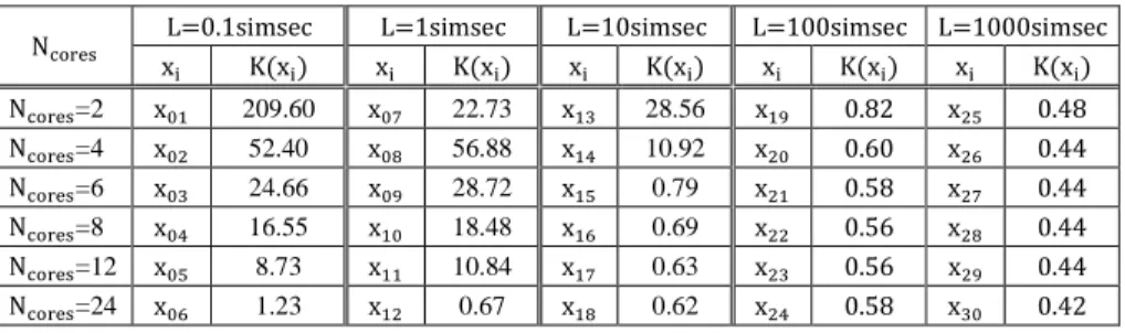
Table 3 shows the costs of simulation experiments 𝐾(𝑥𝑖) (𝑥𝑖∈ 𝑈, 𝑖 = 1,2, … ,30).

Table 3

Cost of PDES simulation experiments K(x_i) [ks]

N_cores L=0.1simsec L=1simsec L=10simsec L=100simsec L=1000simsec

x_i K(x_i) x_i K(x_i) x_i K(x_i) x_i K(x_i) x_i K(x_i)

N_cores=2 x₀₁ 209.60 x₀₇ 22.73 x₁₃ 28.56 x₁₉ 0.82 x₂₅ 0.48

N_cores=4 x₀₂ 52.40 x₀₈ 56.88 x₁₄ 10.92 x₂₀ 0.60 x₂₆ 0.44

N_cores=6 x₀₃ 24.66 x₀₉ 28.72 x₁₅ 0.79 x₂₁ 0.58 x₂₇ 0.44

N_cores=8 x₀₄ 16.55 x₁₀ 18.48 x₁₆ 0.69 x₂₂ 0.56 x₂₈ 0.44

N_cores=12 x₀₅ 8.73 x₁₁ 10.84 x₁₇ 0.63 x₂₃ 0.56 x₂₉ 0.44

In Table 4, values of cost of rules 𝐾(𝑠_𝑗) are shown in order of their occurrence in predictions (𝑠𝑗∈ ⋃8 𝑆𝑡𝑟𝑎𝑖𝑛(𝑖)

𝑖=1 , 𝑗 = 1,2, … ,24).

Table 4 Cost of rules K(s_j) [ks]

s_j s₁ s₂ s₃ s₄ s₅ s₆ s₇ s₈

K(s_j) 313.17 3.70 2.67 2.87 1.85 2.90 0.79 2.29

s_j s₉ s₁₀ s₁₁ s₁₂ s₁₃ s₁₄ s₁₅ s₁₆

K(s_j) 1.63 1.09 0.69 22.74 0.67 1.81 34.90 1.30

s_j s₁₇ s₁₈ s₁₉ s₂₀ s₂₁ s₂₂ s₂₃ s₂₄

K(s_j) 0.79 0.63 2.87 1.09 1.10 1.70 6.68 5.68

In Table 5, costs of predictions 𝐾(𝑆_{𝑡𝑟𝑎𝑖𝑛(𝑖)}) are shown together with the number of prediction rules |𝑆𝑡𝑟𝑎𝑖𝑛(𝑖)| in the prediction (𝑖 = 1,2, … ,8).

Table 5

Cost of predictions K(S_train(i)) [ks] and number of rules in S_train(i)

Prediction(i) 1 2 3 4 5 6 7 8

K(S_train(i)) 331.85 322.97 351.79 357.85 329.67 364.82 336.05 357.99

|S_train(i)| 9 7 10 8 10 10 7 6

In the following points, based on simulation results and on RST modeling and train-and-test examination data, cases of single predictions and series of predictions, with and without dropping, are analyzed using prediction performance coefficients. The basic series of predictions (prediction case 0) is introduced in point 5.2.2. All the other prediction analysis examples (prediction case 1-5) introduced in the analysis are derived from prediction case 0. The efficacy minimum requirement for all prediction cases is 𝐸1_{𝑙𝑖𝑚𝑖𝑡}≥ 60%.

5.2.2 Predictions with Full Set of Attributes and Rules Prediction case 0: ∀_𝑖=1⁸ 𝑆𝑝𝑟𝑒𝑑𝑖𝑐𝑡𝑖𝑜𝑛(𝑖)∶= 𝑆𝑡𝑟𝑎𝑖𝑛(𝑖)

Cost data and rule set sizes for the series of predictions are shown in Table 3, 4 and 5. The effectiveness coefficient of prediction series is

𝐸3𝑠𝑒𝑟𝑖𝑒𝑠= 𝐸3(𝑆𝑡𝑟𝑎𝑖𝑛) = 𝐸28|𝐸18 where 𝐸28=¹₈∑8 𝐸1𝑖

𝑖=1 1

8∑⁸_𝑖=1𝐾(𝑆𝑡𝑟𝑎𝑖𝑛(𝑖)) = 77% 344.12𝑘𝑠⁄ =

⁄ 0.224_𝑘𝑠^% , and

𝐸1₈=¹₈∑⁸_𝑖=1𝐸1(𝑆_{𝑡𝑟𝑎𝑖𝑛(𝑖)})= 77% > (𝐸1_{𝑙𝑖𝑚𝑖𝑡} = 60%).

5.2.3 Dropping in Single Predictions: Efficacy and Efficiency Analysis Prediction case 1: dropping 𝑆𝑝𝑟𝑒𝑑𝑖𝑐𝑡𝑖𝑜𝑛(1)∶= 𝑆_{𝑡𝑟𝑎𝑖𝑛(1)}∖ {𝑠₃}

Set of prediction rules 𝑆𝑡𝑟𝑎𝑖𝑛(1) consists of nine rules (𝑆𝑡𝑟𝑎𝑖𝑛(1)= {𝑠1, 𝑠2, … , 𝑠9}).

The limit 𝐸1𝑙𝑖𝑚𝑖𝑡 ≥ 0.6 has been accepted, thus the rule 𝑠3= (𝑐04(𝑡)⇒ 𝑑01(𝐻)), (𝑠₃∈ 𝑆_{𝑡𝑟𝑎𝑖𝑛(1)}) can be dropped efficaciously since the effect of dropping on 𝐸1 is

(((∑^15=|𝑈_𝑙=1 ^{𝑡𝑒𝑠𝑡(1)|}𝑝(𝑥𝑙))

𝑆_{𝑡𝑟𝑎𝑖𝑛(1)}= 11) − (|𝑀𝑎𝑡𝑐ℎ𝑈_{𝑡𝑒𝑠𝑡(1)}(𝑠₃)| = 2) = 9) ≥ (𝐸1𝑙𝑖𝑚𝑖𝑡∗ |𝑈𝑡𝑒𝑠𝑡(1)| = 0.6 ∗ 15 = 9).

Decision rule 𝑠1= (𝑐04(𝑓)⇒ 𝑑01(𝐿)), (𝑠1∈ 𝑆𝑡𝑟𝑎𝑖𝑛(1)) cannot be dropped efficaciously because

(((∑^15=|𝑈_𝑙=1 ^{𝑡𝑒𝑠𝑡(1)|}𝑝(𝑥𝑙))

𝑆_{𝑡𝑟𝑎𝑖𝑛(1)}= 11) − (|𝑀𝑎𝑡𝑐ℎ𝑈_{𝑡𝑒𝑠𝑡(1)}(𝑠1)| = 3) = 8) ≱ (𝐸1_{𝑙𝑖𝑚𝑖𝑡}∗ |𝑈_{𝑡𝑒𝑠𝑡(1)}| = 0.6 ∗ 15 = 9).

Cost of rule 𝑠3 is 𝐾(𝑠3) = 2.67𝑘𝑠 thus after dropping 𝑠₃ 𝐾(𝑆𝑡𝑟𝑎𝑖𝑛(1)∖ {𝑠3}) = 329.18𝑘𝑠. The efficacy and efficiency coefficients after dropping are

𝐸1(𝑆_{𝑡𝑟𝑎𝑖𝑛(1)}∖ {𝑠₃}) = 60%, 𝐸2(𝑆_{𝑡𝑟𝑎𝑖𝑛(1)}∖ {𝑠₃}) = 0.182_𝑘𝑠^% respectively.

Comparing 𝐸2_{𝑙𝑖𝑚𝑖𝑡} = 𝐸1_{𝑙𝑖𝑚𝑖𝑡}⁄¹₈∑⁸_𝑖=1𝐾(𝑆_{𝑝𝑟𝑒𝑑𝑖𝑐𝑡𝑖𝑜𝑛}) for both before and after dropping cases, the next inequality has been got: 𝐸2_{𝑙𝑖𝑚𝑖𝑡}(𝑆_{𝑡𝑟𝑎𝑖𝑛(1)}) = 0.181_𝑘𝑠^%<

< 𝐸2𝑙𝑖𝑚𝑖𝑡(𝑆𝑡𝑟𝑎𝑖𝑛(1)∖ {𝑠3}) = 0.182_𝑘𝑠^%, that is 𝑆𝑡𝑟𝑎𝑖𝑛(1) is worse in effectiveness.

Prediction case 2: dropping 𝐶𝑝𝑟𝑒𝑑𝑖𝑐𝑡𝑖𝑜𝑛(1)∶= 𝐶 ∖ {𝑐₀₃}

Extending the previous case, the attribute 𝑐03 may be dropped efficaciously if the following set of sufficient conditions can be satisfied:

∃𝑆_𝐸𝐹(1)(𝑆_{𝑡𝑟𝑎𝑖𝑛(1)}= (𝑆_𝐸𝐹(1)∪ 𝑆_𝐹𝐸(1))) ∧ ({𝑐₀₃} ∉ 𝐶_{𝑆𝐸𝐹(1)}) ∧ 𝐸1(𝑆_𝐸𝐹(1)) ≥

≥ 𝐸1𝑙𝑖𝑚𝑖𝑡 , where set 𝐶𝑆_𝐸𝐹(1) denotes the set of condition attributes used by rules of set 𝑆_𝐸𝐹(1). The partitioning 𝑆_{𝑡𝑟𝑎𝑖𝑛(1)}= (𝑆_𝐸𝐹(1)= {𝑠₁, 𝑠₂, 𝑠₃}) ∪ 𝑆_𝐹𝐸(1) = {𝑠₄, 𝑠₅, 𝑠₆, 𝑠₇, 𝑠₈, 𝑠₉}, satisfies the conditions since 𝐸1(𝑆_EF(1)) = 60 % = 𝐸1_{𝑙𝑖𝑚𝑖𝑡} and (𝐶𝑆_𝐹𝐸(1)∖ 𝐶𝑆_𝐸𝐹(1)) = {𝑐03, 𝑐04} ∖ {𝑐₀₄} = {𝑐₀₃}.

The cost of prediction after dropping 𝑐03 is 𝐾(𝑆𝑡𝑟𝑎𝑖𝑛(1)∖{𝑐₀₃}) = 𝐾(𝑆𝐸𝐹(1)) =

= 319.54𝑘𝑠, thus the efficiency got is 𝐸2(𝑆𝑡𝑟𝑎𝑖𝑛(1)∖{𝑐₀₃}) = 0.188_𝑘𝑠^% . 5.2.4 Dropping in Series of Predictions: Effectiveness Analysis Prediction case 3: dropping ∀_𝑖=1⁸ 𝑆𝑝𝑟𝑒𝑑𝑖𝑐𝑡𝑖𝑜𝑛(𝑖)∶= 𝑆𝑡𝑟𝑎𝑖𝑛(𝑖)∖ {𝑠1}

𝐸3𝑠𝑒𝑟𝑖𝑒𝑠= 𝐸3(𝑆𝑡𝑟𝑎𝑖𝑛∖ {𝑠1}) = 𝐸2₈|𝐸18 where

𝐸2₈=¹₈∑⁸_𝑖=1𝐸1_(𝑖)⁄¹₈∑⁸_𝑖=1𝐾(𝑆_{𝑡𝑟𝑎𝑖𝑛(𝑖)}∖ {𝑠₁})= 1.680_𝑘𝑠^% , and 𝐸18=¹₈∑⁸_𝑖=1𝐸1(𝑆𝑡𝑟𝑎𝑖𝑛(𝑖)∖ {𝑠1})= 52%.

In this case, dropping 𝑠1 is highly efficient (since 𝐾(𝑆𝑡𝑟𝑎𝑖𝑛) = 344.12𝑘𝑠 and 𝐾(𝑠1) = 313.17𝑘𝑠 ) but the dropping is not efficacious because 52% <

𝐸1𝑙𝑖𝑚𝑖𝑡 = 60% and thus the dropping is not effective too.

Prediction case 4: dropping ∀_𝑖=1⁸ 𝑆𝑝𝑟𝑒𝑑𝑖𝑐𝑡𝑖𝑜𝑛(𝑖)∶= {𝑠₁, 𝑠₂, 𝑠₃} For the case of this rule dropping effectiveness is

𝐸3_{𝑠𝑒𝑟𝑖𝑒𝑠}= 𝐸3({𝑠₁, 𝑠₂, 𝑠₃}) = 𝐸2₈|𝐸1₈ where 𝐸28=¹₈∑8 𝐸1𝑖

𝑖=1 1

8∑⁸_𝑖=1𝐾(𝑆𝑡𝑟𝑎𝑖𝑛(𝑖)= {𝑠1, 𝑠2, 𝑠3}) =

⁄ 0.194_𝑘𝑠^% , and

𝐸18=¹₈∑⁸_𝑖=1𝐸1(𝑆𝑡𝑟𝑎𝑖𝑛(𝑖)= {𝑠1, 𝑠2, 𝑠3})= 62% > (𝐸1𝑙𝑖𝑚𝑖𝑡= 60%).

Prediction case 5: dropping ∀_𝑖=1⁸ 𝑆𝑝𝑟𝑒𝑑𝑖𝑐𝑡𝑖𝑜𝑛(𝑖)= 𝑆𝑡𝑟𝑎𝑖𝑛(𝑖)|𝐶 ∶=𝐶 ∖ {𝑐₀₃}

Attribute 𝑐03 could be dropped efficaciously for the series of predictions (continuing the analysis of prediction case 2) since the sufficient set of conditions,

⋁8 ∃𝑆𝐸𝐹(𝑖)

𝑖=1 (𝑆𝑡𝑟𝑎𝑖𝑛(i)= (𝑆𝐸𝐹(𝑖)∪ 𝑆𝐹𝐸(𝑖))) ∧ ({𝑐03} ∉ 𝐶_{𝑆𝐸𝐹(𝑖)})) ∧

∧ ((¹₈∑⁸_𝑖=1𝐸1(𝑆_{𝐸𝐹(𝑖)})) ≥ 𝐸1_{𝑙𝑖𝑚𝑖𝑡}), can be satisfied by simply taking

⋁⁸_𝑖=1𝑆_{𝐸𝐹(𝑖)}= {𝑠₁, 𝑠₂, 𝑠₃} for this case too. Thus, the effectiveness evaluation gives the same numbers as for prediction case 4:

𝐸3_{𝑠𝑒𝑟𝑖𝑒𝑠}= 𝐸3(𝑆_𝐸𝐹|𝐶 ∖ {𝑐₀₃}) = 𝐸2₈|𝐸1₈ where 𝐸28=¹₈∑8 𝐸1𝑖

𝑖=1 1

8∑⁸_𝑖=1𝐾(𝑆𝑡𝑟𝑎𝑖𝑛(𝑖)= 𝑆𝐸𝐹(𝑖)) =

⁄ 0.194_𝑘𝑠^% , and

𝐸1₈=¹₈∑⁸_𝑖=1𝐸1(𝑆_{𝐸𝐹(𝑖)})= 62% > (𝐸1_{𝑙𝑖𝑚𝑖𝑡} = 60%).

6 Comparison and Discussion of Predictions

Figure 4 compares three series of predictions 𝑆_{𝑝𝑟𝑒𝑑𝑖𝑐𝑡𝑖𝑜𝑛}= 𝑆_{𝑡𝑟𝑎𝑖𝑛} (case 0), 𝑆𝑝𝑟𝑒𝑑𝑖𝑐𝑡𝑖𝑜𝑛= {𝑠1, 𝑠2, 𝑠3} (case 4) and 𝑆_{𝑝𝑟𝑒𝑑𝑖𝑐𝑡𝑖𝑜𝑛}= 𝑆𝑡𝑟𝑎𝑖𝑛∖ {𝑠1} (case 3). The diagram shows 𝐸1 and 𝐸2 coefficients for every single prediction and shows 𝐸2 and 𝐸1 values of 𝐸3 for the series of predictions too. To make the comparison of predictions easier, the efficiency coefficients are calculated such that 𝐾(𝑆_{𝑝𝑟𝑒𝑑𝑖𝑐𝑡𝑖𝑜𝑛}= {𝑠₁, 𝑠₂, 𝑠₃}) = 319.54𝑘𝑠 = 100%.

For the single predictions of 𝑆𝑝𝑟𝑒𝑑𝑖𝑐𝑡𝑖𝑜𝑛= 𝑆𝑡𝑟𝑎𝑖𝑛 , the relation ∀_𝑖=1⁸ 𝐸1_(𝑖)(𝐸1_(𝑖)≥

≥ 𝐸1𝑙𝑖𝑚𝑖𝑡) is hold, and the relative efficiency of the series 𝐸2 is 72% (𝐸1= 77%).

Figure 4

E1, E2 and E3 evaluation of predictions and droppings

For 𝑆_{𝑝𝑟𝑒𝑑𝑖𝑐𝑡𝑖𝑜𝑛}= {𝑠₁, 𝑠₂, 𝑠₃}, the relation ∀_𝑖=1⁸ 𝐸1_(𝑖)(𝐸1_(𝑖)> 50%) is true for every single prediction. Efficacy of series is 𝐸1 = 62%, with a relative efficiency of 𝐸2 = 62% too. If 𝐸1 = 60% = 𝐸1𝑙𝑖𝑚𝑖𝑡 has been accepted then 𝑆𝑝𝑟𝑒𝑑𝑖𝑐𝑡𝑖𝑜𝑛= {𝑠₁, 𝑠₂, 𝑠₃} performs better: 𝐸2({𝑠₁, 𝑠₂, 𝑠₃}) =60% and 𝐸2(𝑆_{𝑝𝑟𝑒𝑑𝑖𝑐𝑡𝑖𝑜𝑛}= 𝑆_{𝑡𝑟𝑎𝑖𝑛}) =

=56%.

Dropping 𝑠1 (𝑆𝑝𝑟𝑒𝑑𝑖𝑐𝑡𝑖𝑜𝑛= 𝑆𝑡𝑟𝑎𝑖𝑛∖ {𝑠1}) leads to a significant decrease of 𝐸1 (77% → 52%), and results in an ineffective series of predictions. All the single predictions of 𝐸2(𝑆𝑡𝑟𝑎𝑖𝑛∖ {𝑠1}) are in the range between 235% and 1956%. The efficiency of the series 𝐸2(𝑆𝑡𝑟𝑎𝑖𝑛∖ {𝑠1}) is 537%. The rule with the highest cost 𝑠1 has significant influence on efficacy and dominating influence on efficiency of predictions. (Rule 𝑠1 is included in 𝑆𝑝𝑟𝑒𝑑𝑖𝑐𝑡𝑖𝑜𝑛= {𝑠1, 𝑠2, 𝑠3} and its proportion in the cost of the whole set is 98% (Table 4).)

This evaluation indicates the need for the feedback to model identification phase.

The 𝑠1 rule has the form 𝑠1= (𝑐04(𝑓 )⇒ 𝑑01(𝐿)) where 𝑐01(𝑓) = 𝑣^′_𝑐04= 0.1 and 𝑑01(𝐿) = 𝑣^′_𝑑 < 0.6 . The relation 𝑆𝑢𝑝𝑝(𝑠1) = 1 is true for the

77%

71%

62%

52%

1956%

0%

500%

1000%

1500%

2000%

2500%

10%

30%

50%

70%

90%

110%

130%

150%

170%

190%

Prediction(1) Prediction(2) Prediction(3) Prediction(4) Prediction(5) Prediction(6) Prediction(7) Prediction(8) Series coeff.

E1 and E2 values [%]

E1(S(train)) E2(S(train))

E1{s(1), s(2), s(3)} E2{s(1), s(2), s(3)}

E1(S(train)∖{s(1)}) E2(S(train)∖{s(1)})

E2(S(train)\{s1}) values [%]

537%

E3 coefficients

235%

𝑙𝑜𝑜𝑘𝑎ℎ𝑒𝑎𝑑 = 0.1 column in Table 2. The cost of the rule 𝐾(𝑠1) = ∑⁶_𝑙=1𝐾(𝑥𝑙)= 313.17𝑘𝑠 is the sum of costs of 6 experiments of the universe 𝑥₀₁− 𝑥₀₆ in Table 3. It means that if objects 𝑥₀₁− 𝑥₀₆ are excluded from the model, then there is no need for the high cost 𝑠₁ rule.

This modification of the model allows decreasing prediction costs without losing the prediction power in ranges with higher potential speed increases.

Conclusions

In past years, numerous simulation performance prediction methods have been developed that support simulation model development for PDES, since PDES execution can significantly decrease model runtime and developing simulation models with high PDES runtime features have remained challenging tasks. The emerging execution platforms with on-demand access and charge-per-use services bring into focus, the importance of cost/quality evaluation in performance predictions. Here, we have defined prediction performance improvement operations, based on the system of performance coefficients of efficacy (E1), efficiency (E2), effectiveness (E3), characterizing prediction correctness, evaluating correctness to cost relationship and describing correctness cost behavior for a series of predictions, respectively. We included the evaluation and improvement steps in a traditional RST train-and-test algorithm and added it to a classic CFM to form an integrated prediction method. We presented the work of the improved prediction method on a case study of a Closed Queuing Network (CQN) model PDES CFM analysis. In the analysis of the CFM RST model and results of the train-and-test examination, we presented the use of E1, E2 and E3 coefficients for rule and attribute dropping operations and the feedback to the CFM and RST model-identification phase was shown. For the case study implementation, the OMNet++ DES framework and the Rosetta Rough Set Software System were used. Future research is planned to focus on the effectiveness evaluation of simulation model output data, preprocessing for rough modeling and on the application of the method, for methods other than CFM.

References

[1] Perumalla, K. S., (2010) μπ: a Scalable and Transparent System for Simulating MPI Programs, In Proceedings of the 3^rd International ICST Conference on Simulation Tools and Techniques, ICST (Institute for Computer Sciences, Social-Informatics and Telecommunications Engineering), p. 62

[2] Perumalla, K. S., (2006) Parallel and Distributed Simulation: Traditional Techniques and Recent Advances, In Proceedings of the 38^th Winter Simulation Conference, pp. 84-95

[3] D’Angelo, G., (2011) Parallel and Distributed Simulation from Many Cores to the Public Cloud (Extended Version), In: Proceedings of the 2011