AnnotatorJ: an ImageJ plugin to ease hand annotation of cellular compartments

(1)

AnnotatorJ: an ImageJ plugin to ease hand annotation of cellular compartments

ABSTRACT AnnotatorJ combines single-cell identification with deep learning (DL) and man- ual annotation. Cellular analysis quality depends on accurate and reliable detection and seg- mentation of cells so that the subsequent steps of analyses, for example, expression mea- surements, may be carried out precisely and without bias. DL has recently become a popular way of segmenting cells, performing unimaginably better than conventional methods. How- ever, such DL applications may be trained on a large amount of annotated data to be able to match the highest expectations. High-quality annotations are unfortunately expensive as they require field experts to create them, and often cannot be shared outside the lab due to medical regulations. We propose AnnotatorJ, an ImageJ plugin for the semiautomatic anno- tation of cells (or generally, objects of interest) on (not only) microscopy images in 2D that helps find the true contour of individual objects by applying U-Net–based presegmentation.

The manual labor of hand annotating cells can be significantly accelerated by using our tool.

Thus, it enables users to create such datasets that could potentially increase the accuracy of state-of-the-art solutions, DL or otherwise, when used as training data.

INTRODUCTION

Single-cell analysis pipelines begin with an accurate detection of the cells. Even though microscopy analysis software tools aim to become more and more robust to various experimental setups and imaging conditions, most lack efficiency in complex scenarios such as label-free samples or unforeseen imaging conditions (e.g., higher signal-to-noise ratio, novel microscopy, or staining techniques), which opens up a new expectation of such software tools: adaptation ability (Hollandi et al., 2020). Another crucial requirement is to maintain ease of usage and limit the number of parameters the users need to fine-tune to match their exact data domain.

Recently, deep learning (DL) methods have proven themselves worthy of consideration in microscopy image analysis tools as they have also been successfully applied in a wider range of applications

including but not limited to face detection (Sun et al., 2014; Taigman et al., 2014; Schroff et al., 2015), self-driving cars (Redmon et al., 2016;

Badrinarayanan et al., 2017, Grigorescu et al., 2019), and speech recognition (Hinton et al., 2012). Caicedo et al. (Caicedo et al., 2019) and others (Hollandi et al., 2020; Moshkov et al., 2020) proved that single- cell detection and segmentation accuracy can be significantly im- proved utilizing DL networks. The most popular and widely used deep convolutional neural networks (DCNNs) include Mask R-CNN (He et al., 2017): an object detection and instance segmentation network; YOLO (Redmon et al., 2016; Redmon and Farhadi, 2018): a fast object detector; and U-Net (Ronneberger et al., 2015): a fully convolutional network specifically intended for bioimage analysis purposes and mostly used for pixel classification. StarDist (Schmidt et al., 2018) is an instance segmentation DCNN optimal for convex or elliptical shapes (such as nuclei).

As robustly and accurately as they may perform, these networks rely on sufficient data, both in amount and quality, which tends to be the bottleneck of their applicability in certain cases such as single- cell detection. While in more industrial applications (see Grigorescu et al., 2019 for an overview of autonomous driving) a large amount of training data can be collected relatively easily (see the cityscapes dataset [Cordts et al., 2016; available at https://www.cityscapes -dataset.com/] of traffic video frames using a car and camera to

Monitoring Editor Jennifer Lippincott-Schwartz Howard Hughes Medical Institute

Received: Feb 27, 2020 Revised: Jun 24, 2020 Accepted: Jul 17, 2020

This article was published online ahead of print in MBoC in Press (http://www .molbiolcell.org/cgi/doi/10.1091/mbc.E20-02-0156). on July 22, 2020

*Address correspondence to: Péter Horváth (horvath.peter@brc.hu).

© 2020 Hollandi et al. This article is distributed by The American Society for Cell Biology under license from the author(s). Two months after publication it is available to the public under an Attribution–Noncommercial–Share Alike 3.0 Unported Creative Commons License (http://creativecommons.org/licenses/by-nc-sa/3.0).

“ASCB®,” “The American Society for Cell Biology®,” and “Molecular Biology of the Cell®” are registered trademarks of The American Society for Cell Biology.

Abbreviations used: DL, deep learning; DL4J, Deeplearning4j; IoU, intersection over union; ROI, region of interest.

Réka Hollandiâ, Ákos Diósdiâ,b, Gábor Hollandiâ, Nikita Moshkovâ,c,d, and Péter Horváthâ,e,*

aSynthetic and Systems Biology Unit, Biological Research Center, 6726 Szeged, Hungary; ^bDoctoral School of Biology, University of Szeged, 6726 Szeged, Hungary; ^cDoctoral School of Interdisciplinary Medicine, University of Szeged, Koranyi fasor 10, 6720 Szeged, Hungary; ^dNational Research University Higher School of Economics, Faculty of Computer Science, 101000 Moscow, Russia; ^eInstitute for Molecular Medicine Finland, University of Helsinki, 00014 Helsinki, Finland

MBoC | BRIEF REPORT

(2)

record and potentially nonexpert individuals to label the objects), clinical data is considerably more difficult, due to ethical constraints, and expensive to gather as expert annotation is required. Datasets available in the public domain such as BBBC (Ljosa et al., 2012) at https://data.broadinstitute.org/bbbc/, TNBC (Naylor et al., 2017, 2019) or TCGA (Cancer Genome Atlas Research Network, 2008;

Kumar et al., 2017), and detection challenges including ISBI (Coelho et al., 2009), Kaggle (https://www.kaggle.com/, e.g., Data Science Bowl 2018; see at https://www.kaggle.com/c/data-science-bowl -2018), ImageNet (Russakovsky et al., 2015), etc., contribute to the development of genuinely useful DL methods; however, most of them lack heterogeneity of the covered domains and are limited in data size. Even combining them one could not possibly prepare their network/method to generalize well (enough) on unseen domains that vastly differ from the pool they covered. On the contrary, such an adaptation ability can be achieved if the target domain is represented in the training data, as proposed in Hollandi et al., 2020, where synthetic training examples are generated automatically in the target domain via image style transfer.

Eventually, similar DL approaches’ performance can only be in- creased over a certain level if we provide more training examples.

The proposed software tool was created for this purpose: the expert can more quickly and easily create a new annotated dataset in their desired domain and feed the examples to DL methods with ease.

The user-friendly functions included in the plugin help organize data and support annotation, for example, multiple annotation types, editing, classes, etc. Additionally, a batch exporter is provided offering different export formats matching typical DL models’; supported annotation and export types are visualized in Figure 1; open-source code is available at https://github.com/spreka/annotatorj under GNU GPLv3 license.

We implemented the tool as an ImageJ (Abramoff et al., 2004, Schneider et al., 2012) plugin because ImageJ is frequently used by bioimage analysts, providing a familiar environment for users. While

x,y,width,height 9,20,26,23 41,4,33,23 91,7,18,21 31,41,32,21 2,69,26,24 29,82,28,19 81,41,22,19 86,66,29,21 79,101,21,9 53,107,9,3 116,11,4,22

.csv

coordinates

1 2 3

4

5 6

7 8 10 9

11

multi-layer (stack)

z-stack z

multi-label binary

export semantic

instance bbox

annotation original

FIGURE 1: Annotation types. The top row displays our supported types of annotation: instance, semantic, and bounding box (noted as “bbox” in the figure) based on the same objects of interest, in this case nuclei, shown in red. Instances mark the object contours, semantic overlay shows the regions (area) covered, while bounding boxes are the smallest enclosing rectangles around the object borders. Export options are shown in the bottom row: multilabel, binary, multilayer images, and coordinates in a text file. Lines mark the supported export options for each annotation type by colors: orange for instance, green for semantic, and blue for bounding box. Dashed lines indicate additional export options for semantics that should be used carefully.

other software also provide a means to support annotation, for example, by machine learning–based pixel classification (see a detailed comparison in Materials and Methods), AnnotatorJ is a lightweight, free, open-source, cross-platform alternative. It can be easily installed via its ImageJ update site at https://sites.imagej.net/Spreka/ or run as a standalone ImageJ instance con- taining the plugin.

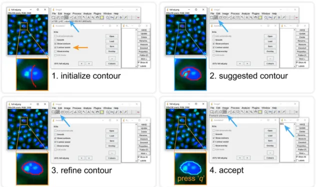
In AnnotatorJ we initialize annotations with DL presegmentation using U-Net to suggest contours from as little as a quickly drawn line over the object (see Supplemen- tal Material and Figure 2). U-Net predicts pixels belonging to the target class with the highest probability within a small bounding box (a rectangle) around the initially drawn contour; then a fine approximation of the true object boundary is calculated from connected pixels; this is referred to as the suggested contour. The user then manually refines the contour to create a pixel-perfect annotation of the object.

RESULTS AND DISCUSSION Performance evaluation

We quantitatively evaluated annotation performance and speed in AnnotatorJ (see Figures 3 and 4) with the help of three annotators who had experience in cellular compartment annotation. Both annotation accuracy and time were measured on the same two test sets: a nucleus and a cytoplasm image set (see also Supplemental Figure S1 and Supplemental Material). Both test sets contained images of various experimental conditions, including fluo- rescently labeled and brightfield-stained samples, tissue section, and cell culture images. We compared the effectiveness of our plugin using Contour assist mode to only allowing the use of Automatic adding. Even though the latter is also a functionality of AnnotatorJ, it ensured that the measured annotation times correspond to a single object each. Without this option the user must press the key “t” after every contour drawn to add it to the region of interest (ROI) list, which can be unintendedly missed, increasing its time as the same contour must be drawn again.

For the annotation time test presented in Figure 3 we measured the time passed between adding new objects to the annotated object set in ROI Manager for each object, then averaged the times for each image and each annotator, respectively. Time was measured in the Java implementation of the plugin in milliseconds. Figures 3 and 4 show SEM error bars for each mean measurement (see Supple- mental Material for details).

In the case of annotating cell nuclei, results confirm that hand- annotation tasks can be significantly accelerated using our tool.

Each of the three annotators were faster by using Contour assist;

two of them nearly double their speed.

To ensure efficient usage of our plugin in annotation assistance, we also evaluated the accuracies achieved in each test case by cal- culating mean intersection over union (IoU) scores of the annotations as segmentations compared with ground truth masks previously created by different expert annotators. We used the mean IoU score defined in the Data Science Bowl 2018 competition (https://

www.kaggle.com/c/data-science-bowl-2018/overview/evaluation) and in Hollandi et al., 2020:

(3)

FIGURE 2: Contour assist mode of AnnotatorJ. The blocks show the order of steps; the given tool needed is

automatically selected. User interactions are marked with orange arrows, and automatic steps with blue. 1) Initialize the contour with a lazily drawn line; 2) the suggested contour appears (a window is shown until processing completes), brush selection tool is selected automatically; 3) refine the contour as needed; 4) accept it by pressing the key “q” or reject with “Ctrl” + “delete.” Accepting adds the ROI to ROI Manager with a numbered label. See also Supplemental Material for a demo video (figure2.mov).

Expert #1 Expert #2 Expert #3

annotator 0

2000 4000 6000 8000 10000 12000 14000 16000 18000

time (ms)

Nuclei annotation time

auto adding contour assist

A B

C

FIGURE 3: Annotation times on nucleus images. AnnotatorJ was tested on sample microscopy images (both fluorescent and brightfield, as well as cell culture and tissue section images);

annotation time was measured on a per-object (nucleus) level. Bars represent the mean annotation times on the test image set; error bars show SEM. Orange corresponds to Contour assist mode and blue to only allowing the Automatic adding option. (A) Nucleus test set annotation times. (B) Example cell culture test images. (C) Example histopathology images.

Images shown in B and C are 256 × 256 crops of original images. Some images are courtesy of Kerstin Elisabeth Dörner, Andreas Mund, Viktor Honti, and Hella Bolck.

t t

t t t

IoUscore TP

TP FP FN

( ) ( )

( ) ( ) ( )

= + + + ε (1)

IoU determines the overlapping pixels of the segmented mask with the ground truth mask (intersection) compared with their union. The IoU score is calculated at 10 different thresholds from 0.5 to 0.95 with 0.05 steps; at each threshold true positive (TP), false positive (FP), and false negative (FN) objects are counted. An object is considered TP if its IoU is greater than the given threshold t. IoU scores calculated at all 10 thresholds were finally averaged to yield a single IoU score for a given image in the test set.

An arbitrarily small ε = 10^–40 value was added to the denominators for numerical stability. Equation 1 is a modified version of mean average precision (mAP) typically used to describe the accuracy of instance segmentation approaches. Precision is for- mulated as

t t

precision

TP FP

( ) ( )

= + + ε

TP (2)

Nucleus and cytoplasm image segmentation accuracies were averaged over the test sets, respectively. We compared our

(4)

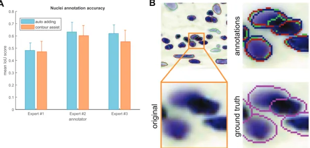
annotators using and not using Contour assist mode (Figure 4). The results show greater interexpert than intraexpert differences, allowing us to conclude that the annotations created in AnnototarJ are nearly as accurate as freehand annotations.

Export evaluation

As the training data annotation process for deep learning applications requires the annotated objects to be exported in a manner that DL models can load them, which typically covers the four types of export options offered in AnnotatorJExporter, it is also important to investigate the efficiency of export. We measured export times similarly to annotation times. For the baseline results, each object defined by their ROI was copied to a new empty image, then filled and saved to create a segmentation mask image file. Exportation from Annota- torJExporter was significantly faster and only required a few clicks: it took four orders of magnitude less time to export the annotations (∼60 ms). Export times reported correspond to a randomly selected expert so that computer hardware specifications remain the same.

Comparison to other tools and software packages

The desire to collect annotated datasets has arisen with the growing popularity and availability of application-specific DL methods. Ob- ject classification on natural images (photos) and face recognition are frequently used examples of such applications in computer vision. We discuss some of the available software tools created for image annotation tasks and compare their feature scope in the following table (Table 1; see also Supplemental Table S1) and in the Supplemental Material.

We collected our list of methods to compare following Mori- kawa, 2019 and “The best image annotation platforms”, 2018.

While there certainly is a considerable amount of annotation tools for object detection purposes, most of them are not open source.

We included Lionbridge.AI (https://lionbridge.ai/services/image -annotation/) and Hive (https://thehive.ai/), two service-based solutions, because of their wide functionality and artificial intelligence support. Both of them work in a project-management way and out- source the annotation task to enable fast and accurate results. Their

main application spectra cover more general object detection tasks like classification of traffic video frames. LabelImg (https://github .com/tzutalin/labelImg), on the other hand, as well as the following tools, is open source but offers a narrower range of annotation options and lacks machine learning support making it a lightweight but free alternative. VGG Image Annotator (Dutta and Zisserman, 2019) comes on a web-based platform, therefore making it very easy for the user to become familiarized with the software. It enables multiple types of annotation with class definition. Diffgram (https://

diffgram.com/) is available both online and as a locally installable version (Python) and adds DL support which speeds up the annotation process significantly; that is, provided the intended object classes are already trained and the DL predictions only need minor edit. A similar, also web-based approach is provided by supervise.ly (https://supervise.ly/; see the Supplemental Material), which is free for research purposes. Even though web-hosted services offer a convenient solution for training new models (if supported), handling sen- sitive clinical data may be problematic. Hence, locally installable software is more desirable in biological and medical applications. A software closer to the bioimage analyst community is CytoMine (Marée et al., 2016; Rubens et al., 2019), a more general image processing tool with a lot of annotation options that also provides DL support and has a web interface. SlideRunner (Aubreville et al., 2018) was created for large tissue section (slide) annotation specifically, but similar to others it does not integrate machine learning methods to help annotation and rather focuses on the classification task.

AnnotatorJ, on the other hand, as an ImageJ (Fiji) plugin should provide a familiar environment for bioimage annotators to work in.

It offers all the functionality available in similar tools (such as different annotation options: bounding box, polygon, freehand drawing, semantic segmentation, and editing them) while it also incorporates support for a popular DL model, U-Net. Furthermore, any user- trained Keras model can be loaded into the plugin with ease because of the DL4J framework, extending its use cases to general object annotation tasks (see Supplemental Figure S2 and Supple- mental Material). Due to its open-source implementation, the users can modify or extend the plugin to even better fit their needs.

A

Expert #1 Expert #2 Expert #3

annotator 0

0.1 0.2 0.3 0.4 0.5 0.6 0.7 0.8

mean IoU score

Nuclei annotation accuracy auto adding

contour assist

annotation s ground trut h

original

B

FIGURE 4: Annotation accuracies. Annotations created in the same test as the times measured in Figure 3 were evaluated using mean IoU scores for the nucleus test set. Error bars show SEM; colors are as in Figure 3. (A) Nucleus test set accuracies. (B) Example contours drawn by our expert annotators. Inset highlighted in orange is zoomed in showing the original image; annotations are marked in red, green, and blue corresponding to experts #1–3, respectively, and ground truth contours (in magenta) are overlayed on the original image for comparison.

(5)

Additionally, as an ImageJ plugin it requires no software installation, can be downloaded inside ImageJ/Fiji (via its update site, https://

sites.imagej.net/Spreka/), or run as a standalone ImageJ instance with this plugin.

We also briefly discuss ilastik (Sommer et al., 2011; Berg et al., 2019) and Suite2p (Pachitariu et al., 2017) in the Supplemental Ma- terial because they are not primarily intended for annotation purposes. Two ImageJ plugins that offer manual annotation and machine learning–generated outputs, Trainable Weka Segmentation (Arganda-Carreras et al., 2017) and LabKit (Arzt, 2017), are also detailed in the Supplemental Material.

We presented an ImageJ plugin, AnnotatorJ, for convenient and fast annotation and labeling of objects on digital images. Multiple export options are also offered in the plugin.

We tested the efficiency of our plugin with three experts on two test sets comprising nucleus and cytoplasm images. We found that our plugin accelerates the hand-annotation process on average and offers up to four orders of magnitude faster export. By integrating the DL4J Java framework for U-Net contour suggestion in Contour assist mode any class of object can be annotated easily: the users can load their own custom models for the target class.

MATERIALS AND METHODS Motivation

We propose AnnotatorJ, an ImageJ (Abramoff et al., 2004, Schnei- der et al., 2012) plugin for the annotation and export of cellular compartments that can be used to boost DL models’ performance.

The plugin is mainly intended for bioimage annotation but could possibly be used to annotate any type of object on images (see Supplemental Figure S2 for a general example). During development we kept in mind that the intended user should be able to get comfortable with the software very quickly and quicken the otherwise truly time-consuming and exhausting process of manually annotating single cells or their compartments (such as individual nucle- oli, lipid droplets, nucleus, or cytoplasm).

The performance of DL segmentation methods is significantly influenced by both the training data size and its quality. Should we feed automatically segmented objects to the network, errors pres- ent in the original data will be propagated through the network during training and bias the performance, hence such training data should always be avoided. Hand-annotated and curated data, however, will minimize the initial error boosting the expected performance increase on the target domain to which the annotated data belongs. NucleAIzer (Hollandi et al., 2020) showed an increase in nucleus segmentation accuracy when a DL model was trained on synthetic images generated from ground truth annotations instead of presegmented masks.

Features

AnnotatorJ helps organize the input and output files by automatically creating folders and matching file names to the selected type and class of annotation. Currently, the supported annotation types are 1) instance, 2) semantic, and 3) bounding box (see Figure 1). Each of these are typical inputs of DL networks; instance annotation provides individual objects separated by their boundaries (useful in the case of, e.g., clumped cells of cancerous regions) and can be used to provide training data for instance segmentation networks such as Mask R-CNN (He et al., 2017). Semantic annotation means foreground–background separation of the image without distinguishing individual objects (foreground); a typical architecture using such segmentations is U-Net (Ronneberger et al., 2015). And finally, bounding box annotation is done by identifying the object’s bounding

Feature

Tool LabelImgLionbridge.AIHiveVGG Image AnnotatorDiffgramCytoMineSlideRunnerAnnotatorJ Open source✓××✓✓✓✓✓ Cross-platform✓serviceservice✓✓Ubuntu✓✓ ImplementationPythonN/AN/AwebPython, webDocker, webPythonJava Annotation

Bounding box✓✓✓✓✓✓✓✓ Freehand ROI×xN/A××✓×✓ Polygonal region×✓✓✓✓✓✓✓ (ImageJ) Semantic×✓✓××✓×✓ Single clicka×××××✓ (magic wand)✓✓ (drag) Edit selectionx (drag)N/AN/A✓✓✓N/A✓ Class option✓✓✓✓✓✓✓✓ DLSupport×AI assistN/A×✓✓×✓ Model import×N/AN/A×TensorflowN/A×Keras, DL4J aBounding box drawing with a single click and drag is not considered a single click annotation. TABLE 1: Comparison of annotation software tools.

(6)

rectangle, and is generally used in object detection networks (like YOLO [Redmon et al., 2016] or R-CNN [Girshick et al., 2014]).

Semantic annotation is done by painting areas on the image overlay. All necessary tools to operate a given function of the plugin are selected automatically. Contour or overlay colors can be selected from the plugin window. For a detailed description and user guide please see the documentation of the tool (available at https://

github.com/spreka/annotatorj repository).

Annotations can be saved to default or user-defined “classes”

corresponding to biological phenotypes (e.g., normal or cancerous) or object classes—used as in DL terminology (such as person, chair, bicycle, etc.), and later exported in a batch by class. Phenotypic dif- ferentiation of objects can be supported by loading a previously annotated class’s objects for comparison as overlay to the image and toggling their appearance by a checkbox.

We use the default ImageJ ROI Manager to handle instance annotations as individual objects. Annotated objects can be added to the ROI list automatically (without the bound keystroke “t” as defined by ROI Manager) when the user releases the mouse button used to draw the contour by checking its option in the main window of the plugin. This ensures that no annotation drawn is missing from the ROI list.

Contour editing is also possible in our plugin using “Edit mode”

(by selecting its checkbox) in which the user can select any already annotated object on the image by clicking on it, then proceed to edit the contour and either apply modifications with the shortcut

“Ctrl” + “q,” discard them with “escape,” or delete the contour with

“Ctrl” + “delete.” The given object selected for edit is highlighted in inverse contour color.

Object-based classification is also possible in “Class mode” (via its checkbox): similarly to “Edit mode,” ROIs can be assigned to a class by clicking on them on the image which will also update the selected ROI’s contour to the current class’s color. New classes can be added and removed, and their class color can be changed. A default class can be set for all unassigned objects on the image.

Upon export (using either the quick export button “[^]” in the main window or the exporter plugin) masks are saved by classes.

In the options (button “…” in the main window) the user can select to use either U-Net or a classical region-growing method to initialize the contour around the object marked. Currently only instance annotation can be assisted.

Contour suggestion using U-Net

Our annotation helper feature “Contour assist” (see Figure 2) allows the user to work on initialized object boundaries by roughly marking an object’s location on the image which is converted to a well-defined object contour via weighted thresholding after a U-Net (Ron- neberger et al., 2015) model trained on nucleus or other compartment data predicts the region covered by the object. We refer to this as the suggested contour and expect the user to refine the boundaries to match the object border precisely. The suggested contour can be further optimized by applying active contour (AC;

Kass et al., 1988) to it. We aim to avoid fully automatic annotation (as previously argued) by only enabling one object suggestion at a time and requiring manual interaction to either refine, accept, or reject the suggested contour. These operations are bound to key- board shortcuts for convenience (see Figure 2). When using the Contour assist function automatic adding of objects is not available to encourage the user to manually validate and correct the suggested contour as needed.

In Figure 2 we demonstrate Contour assist using a U-Net model trained on versatile microscopy images of nuclei in Keras and on a

fluorescent microscopy image of a cell culture where the target objects, nuclei, are labeled with DAPI (in blue). This model is provided at https://github.com/spreka/annotatorj/releases/tag/v0.0.2-model in the open-source code repository of the plugin.

Contour suggestions can be efficiently used for proper initializa- tion of object annotation, saving valuable time for the expert annotator by suggesting a nearly perfect object contour that only needs refinement (as shown in Figure 2). Using a U-Net model accurate enough for the target object class, the expert can focus on those image regions where the model is rather uncertain (e.g., around the edges of an object or the separating line between adja- cent objects) and fine-tune the contour accurately while sparing considerable effort on more obvious regions (like an isolated object on simple background) by accepting the suggested contour after marginal correction.

The framework of the chosen U-Net implementation, DL4J (available at http://deeplearning4j.org/ or https://github.com/

eclipse/deeplearning4j), supports Keras model import, hence custom, application-specific models can be loaded in the plugin easily by either training them in DL4J (Java) or Python (Keras) and saving the trained weights and model configuration in .h5 and .json files.

This vastly extends the possible fields of application for the plugin to general object detection or segmentation tasks (see Supplemen- tal Material and Supplemental Figures S2 and S3).

Exporter

The annotation tool is supplemented by an exporter, AnnotatorJ- Exporter plugin, also available in the package. It was optimized for the batch export of annotations created by our annotation tool.

For consistency, one class of objects can be exported at a time.

We offer four export options: 1) multilabeled, 2) multilayered, 3) semantic images, and 4) coordinates (see Figure 1). Instance annotations are typically expected to be exported as multilabeled (instance-aware) or multilayered (stack) grayscale images, the latter of which is useful for handling overlapping objects such as cy- toplasms in cell culture images. Semantic images are binary foreground–background images of the target objects while coordinates (top-left corner [x,y] of the bounding rectangle appended by its width and height in pixels) can be useful training data for object detection applications including astrocyte localization (Suley- manova et al., 2018) or in a broader aspect, face detection (Taig- man et al., 2014). All export options are supported for semantic annotation; however, we note that in instance-aware options (multilabeled or multilayered mask and coordinates) only such objects are distinguished whose contours do not touch on the annotation image.

OpSeF compatibility

OpSeF (Open Segmentation Framework; Rasse et al., 2020) is an interactive python notebook-based framework (available at https://

github.com/trasse/OpSeF-IV) that allows users to easily try different DL segmentation methods in customizable pipelines. We extended AnnotatorJ to support the data structure and format used in OpSeF to allow seamless integration in these pipelines, so users can manually modify, create, or classify objects found by OpSeF in Annota- torJ, then export the results in a compatible format for further use in the former software. A user guide is provided in the documentation of https://github.com/trasse/OpSeF-IV.

ImageJ

ImageJ (or Fiji: Fiji is just ImageJ; Schindelin et al., 2012) is an open- source, cross-platform image analysis software tool in Java that has

(7)

been successfully applied in numerous bioimage analysis tasks (segmentation [Legland et al., 2016; Arganda-Carreras et al., 2017], par- ticle analysis [Abramoff et al. 2004], etc.) and is supported by a broad range of community, comprising of biomage analyst end users and developers as well. It provides a convenient framework for new developers to create their custom plugins and share them with the community. Many typical image analysis pipelines have already been implemented as a plugin, for example, U-Net segmentation plugin (Falk et al., 2019) or StarDist segmentation plugin (Schmidt et al., 2018).

U-Net implementation

We used the DL4J (http://deeplearning4j.org/) implementation of U-Net in Java. DL4J enables building and training custom DL networks, preparing input data for efficient handling and supports both GPU and CPU computation throughout its ND4J library.

The architecture of U-Net was first developed by Ronneberger et al. (Ronneberger et al., 2015) and was designed to learn medical image segmentation on a small training set when a limited amount of labeled data is available, which is often the case in biological contexts. To handle touching objects as often is the case in nuclei segmentation, it uses a weighted cross entropy loss function to en- hance the object-separating background pixels.

Region growing

A classical image processing algorithm, region growing (Haralick and Shapiro, 1985; Adams and Bischof, 1994) starts from initial seed points or objects and expands the regions towards the object boundaries based on the intensity changes on the image and constraints on distance or shape. We used our own implementation of this algorithm.

ACKNOWLEDGMENTS

R.H., N.M., A.D., and P.H. acknowledge support from the LENDU- LET-BIOMAG grant (Grant no. 2018-342), from the European Regional Development Funds (GINOP-2.3.2-15-2016-00006, GINOP-2.3.2-15-2016-00026, and GINOP-2.3.2-15-2016-00037), from the H2020-discovAIR (874656), and from Chan Zuckerberg Ini- tiative, Seed Networks for the HCA-DVP. We thank Krisztián Koós for the technical help, and Máté Görbe and Tamás Monostori for testing the plugin.

REFERENCES

The best image annotation platforms for computer vision (2018, October 30).

+ an honest review of each, https://hackernoon.com/the-best-image -annotation-platforms-for-computer-vision-an-honest-review-of-each -dac7f565fea.

Abramoff MD, Magalhaes PJ, Ram SJ (2004). Image processing with Im- ageJ. Biophoton Int, 11, 36–42.

Adams R, Bischof L (1994). Seeded region growing, IEEE Trans Pattern Anal Mach Intell 16, 641–647.

Arganda-Carreras I, Kaynig V, Rueden C, Eliceiri KW, Schindelin J, Cardona A, Sebastian Seung H (2017). Trainable Weka segmentation: a machine learning tool for microscopy pixel classification. Bioinformatics 33, 2424–2426.

Arganda-Carreras I, Turaga SC, Berger DR, Cires˛an D, Giusti A, Gambardella LM, Schmidhuber J, Laptev D, Dwivedi S, Buhmann JM, et al. (2015).

Crowdsourcing the creation of image segmentation algorithms for con- nectomics. Front Neuroanat 9, 142.

Arzt M (2017). https://imagej.net/Labkit.

Aubreville M, Bertram C, Klopfleisch R, Maier A (2018). SlideRunner. In:

Bildverarbeitung für die Medizin 2018, Heidelberg, Berlin: Informatik aktuell, Springer Vieweg, pp. 309–314. https://doi.org/10.1007/978-3 -662-56537-7_81.

Badrinarayanan V, Kendall A, Cipolla R (2017). SegNet: a deep convolutional encoder-decoder architecture for image segmentation. IEEE Trans Pattern Anal Mach Intell 39, 2481–2495.

Berg S, Kutra D, Kroeger T, StraehleCN, KauslerBX, HauboldC, SchieggM, AlesJ, BeierT, RudyM, et al. (2019). ilastik: interactive machine learning for (bio)image analysis. Nat Methods 16, 1226–1232.

Caicedo JC, Roth J, Goodman A, Becker T, Karhohs KW, Broisin M, Molnar C,BeckerT, KarhohsKW, BroisinM, et al. (2019). Evaluation of deep learning strategies for nucleus segmentation in fluorescence images.

Cytometry A 95, 952–965.

Cancer Genome Atlas Research Network (2008). Comprehensive genomic characterization defines human glioblastoma genes and core pathways.

Nature 455, 1061–1068.

Coelho LP, Shariff A, Murphy RF (2009). Nuclear segmentation in mi- croscope cell images: a hand-segmented dataset and comparison of algorithms. 2009 IEEE International Symposium on Biomedical Imaging: From Nano to Macro. Available at https://doi.org/10.1109/

isbi.2009.5193098.

Cordts M, Omran M, Ramos S, Rehfeld T, Enzweiler M, Benenson R, Franke U, Roth S, Schiele B, et al. (2016). The cityscapes dataset for semantic urban scene understanding. In 2016 IEEE Conference on Computer Vision and Pattern Recognition (CVPR). Available at https://

doi.org/10.1109/cvpr.2016.350.

Dutta A, Zisserman A (2019). The VIA annotation software for images, audio and video. In Proceedings of the 27th ACM International Conference on Multimedia - MM ‘19. Available at https://doi.

org/10.1145/3343031.3350535.

Eclipse Deeplearning4j Development Team. Deeplearning4j: open-source distributed deep learning for the JVM, Apache Software Foundation License 2.0. http://deeplearning4j.org

Falk T, Mai D, Bensch R, Çiçek Ö, Abdulkadir A, Marrakchi Y, Böhm A, Deubner J, Jäckel Z, Seiwald K, et al. (2019). U-Net: deep learning for cell counting, detection, and morphometry. Nat Methods 16, 67–70.

Frank E, Hall MA, Witten IH (2016). “The WEKA Workbench”, online appen- dix for Data Mining: Practical Machine Learning Tools and Techniques, 4th ed., Morgan Kaufmann.

Girshick R, Donahue J, Darrell T, Malik J (2014). Rich feature hierarchies for accurate object detection and semantic segmentation. In 2014 IEEE Conference on Computer Vision and Pattern Recognition. Available at https://doi.org/10.1109/cvpr.2014.81.

Grigorescu S, Trasnea B, Cocias T, Macesanu G (2019). A survey of deep learning techniques for autonomous driving. J Field Rob 37, 362–386.

Haralick RM, Shapiro LG (1985). Image segmentation techniques.

Applications of Artificial Intelligence II. Available at https://doi.

org/10.1117/12.948400.

He K, Gkioxari G, Dollar P, Girshick R (2017). Mask R-CNN. In 2017 IEEE In- ternational Conference on Computer Vision (ICCV). Available at https://

doi.org/10.1109/iccv.2017.322.

Hinton G, Deng L, Yu D, Dahl G, Mohamed A-R, Jaitly N, Senior A, Vanhoucke V, Nguyen P, Sainath TN, et al. (2012). Deep neural networks for acoustic modeling in speech recognition: the shared views of four research groups. IEEE Signal Process Mag 29, 82–97.

Hollandi R, Szkalisity A, Toth T, Tasnadi E, Molnar C, Mathe B, Grexa I, Molnar J, Balind A, Gorbe M, et al. (2020). nucleAIzer: a parameter-free deep learning framework for nucleus segmentation using image style transfer. Cell Syst 10, 453–458.e6.

Kass M, Witkin A, Terzopoulos D (1988). Snakes: active contour models.

Int J Comput Vis 1, 321–331.

Kumar N, Verma R, Sharma S, Bhargava S, Vahadane A, Sethi A (2017). A dataset and a technique for generalized nuclear segmentation for com- putational pathology. IEEE Trans Med Imaging 36, 1550–1560.

Legland D, Arganda-Carreras I, Andrey P (2016). MorphoLibJ: integrated library and plugins for mathematical morphology with ImageJ. Bioinfor- matics 32, 3532–3534.

Ljosa V, Sokolnicki KL, Carpenter AE (2012). Annotated high-throughput microscopy image sets for validation. Nat Methods 9, 637.

Marée R, Rollus L, Stévens B, Hoyoux R, Louppe G, Vandaele R, Begon J-M, Kainz P, Geurts P, Wehenkel L, et al. (2016). Collaborative analysis of multi- gigapixel imaging data using Cytomine. Bioinformatics 32, 1395–1401.

Morikawa R (July 18, 2019). 24 best image annotation tools for computer vision. Available at https://lionbridge.ai/articles/image-annotation-tools- for-computer-vision/.

Moshkov N, Mathe B, Kertesz-Farkas A, Hollandi R, Horvath P (2020).

Test-time augmentation for deep learning-based cell segmentation on microscopy images. Sci Rep 10, 5068.

Naylor P, Lae M, Reyal F, Walter T (2017). Nuclei segmentation in histopathology images using deep neural networks. In 2017 IEEE 14th International Symposium on Biomedical Imaging (ISBI 2017). Available at https://doi.org/10.1109/isbi.2017.7950669.

(8)

Naylor P, Lae M, Reyal F, Walter T (2019). Segmentation of nuclei in histopathology images by deep regression of the distance map. IEEE Trans Med Imaging 38, 448–459.

Pachitariu M, Stringer C, Dipoppa M, Schröder S, Rossi LF, Dalgleish H, Carandini M, (2017). Suite2p: beyond 10,000 neurons with standard two-photon microscopy. BioRxiv. https://doi.org/10.1101/061507.

Rasse TM, Hollandi R, Horvath P (2020). OpSeF IV: open source Python framework for segmentation of biomedical images. BioRxiv. https://doi .org/10.1101/2020.04.29.068023.

Redmon J, Divvala S, Girshick R, Farhadi A (2016). You only look once:

unified, real-time object detection. In 2016 IEEE Conference on Computer Vision and Pattern Recognition (CVPR). Available at https://

doi.org/10.1109/cvpr.2016.91.

Redmon J, Farhadi A (2018). YOLOv3: an incremental improvement. arXiv https://arxiv.org/abs/1804.02767.

Ronneberger O, Fischer P, Brox T (2015). U-Net: convolutional networks for biomedical image segmentation. In Lecture Notes in Computer Science, Springer, Vol. 9351, 234–241.

Rubens U, Hoyoux R, Vanosmael L, Ouras M, Tasset M, Hamilton C, Longuespée R, Marée R (2019). Cytomine: toward an open and collaborative software platform for digital pathology bridged to molecular investigations. Prot Clin Appl 13, 1800057.

Russakovsky O, Deng J, Su H, Krause J, Satheesh S, Ma S, Huang Z, Karpathy A, Khosla A, Bernstein M, et al. (2015). ImageNet large scale visual recognition challenge. Int J Comput Vis, 115, 211–252.

Schindelin J, Arganda-Carreras I, Frise E, Kaynig V, Longair M, Pietzsch T, Preibisch S, Rueden C, Saalfeld S, Schmid B, et al. (2012). Fiji: an open- source platform for biological-image analysis. Nat Methods 9, 676–682.

Schmidt U, Weigert M, Broaddus C, Myers G (2018). Cell detection with star-convex polygons. In Lecture Notes in Computer Science, Springer, 265–273. Crossref. Web.

Schneider CA, Rasband WS, Eliceiri KW (2012). NIH image to ImageJ:

25 years of image analysis. Nat Methods 9, 671–675.

Schroff F, Kalenichenko D, Philbin J (2015). FaceNet: a unified embed- ding for face recognition and clustering. In 2015 IEEE Conference on Computer Vision and Pattern Recognition (CVPR), pp. 815–823. doi:

10.1109/CVPR.2015.7298682.

Sommer C, Straehle C, Kothe U, Hamprecht FA (2011). Ilastik: interactive learning and segmentation toolkit. In IEEE International Symposium on Biomedical Imaging: From Nano to Macro 2011, 230–233.

Suleymanova I, Balassa T, Tripathi S, Molnar C, Saarma M, Sidorova Y, Horvath P (2018). A deep convolutional neural network approach for astrocyte detection. Sci Rep 8, 12878.

Sun Y, Wang X, Tang X, (2014). Deep learning face representation from predicting 10,000 classes. In 2014 IEEE Conference on Computer Vision and Pattern Recognition, pp. 1891–-1898. doi: 10.1109/CVPR.2014.244.

Taigman Y, Yang M, Ranzato M’A, Wolf L (2014). DeepFace: closing the gap to human-level performance in face verification. In 2014 IEEE Confer- ence on Computer Vision and Pattern Recognition. Available at https://

doi.org/10.1109/cvpr.2014.220.