Order Book Modeling
?Viktor Burj´an and B´alint Gyires-T´oth Budapest University of Technology and Economics Department of Telecommunications and Media Informatics
burjan.viktor@gmail.com, toth.b@tmit.bme.hu
Abstract. Financial processes are frequently explained by econometric models, however, data-driven approaches may outperform the analytical models with adequate amount and quality data and algorithms. In the case of today’s state-of-the-art deep learning methods the more data leads to better models. However, even if the model is trained on massively parallel hardware, the preprocessing of a large amount of data is usually still done in a traditional way (e.g. few hundreds of threads on Central Processing Unit, CPU).
In this paper, we propose a GPU accelerated pipeline, which assesses the burden of time taken with data preparation for machine learning in financial applications. With the reduced time, it enables its user to ex- periment with multiple parameter setups in much less time. The pipeline processes and models a specific type of financial data – limit order books – on massively parallel hardware. The pipeline handles data collection, order book preprocessing, data normalisation, and batching into train- ing samples, which can be used for training deep neural networks and inference. Time comparisons of baseline and optimized approaches are part of this paper.
Keywords: financial modeling·limit order book·deep learning·mas- sively parallel
?The research presented in this paper has been supported by the European Union, co-financed by the European Social Fund (EFOP-3.6.2-16-2017-00013, Thematic Fundamental Research Collaborations Grounding Innovation in Informatics and Infocommunications), by the BME-Artificial Intelligence FIKP grant of Ministry https://www.overleaf.com/project/5e458316e0c5bc0001c37283of Human Resources (BME FIKP-MI/SC), by Doctoral Research Scholarship of Ministry of Human Re- sources ( ´UNKP-19-4-BME-189) in the scope of New National Excellence Program, by J´anos Bolyai Research Scholarship of the Hungarian Academy of Sciences. We gratefully acknowledge the support of NVIDIA Corporation with the donation of the Titan V GPU used for this research.
1 Introduction
A limit order book (LOB) contains the actual buy and sell limit orders that exists on a financial exchange at a given time.1 Every day on major exchanges, like New York Stock Exchange, the volume of clients’ orders can be tremendous, and each of them has to be processed and recorded in the order book. Deep learning models are capable of representation learning and modeling jointly [2], thus, other machine learning methods (which requires roboust feature engineer- ing) can be outperformed in case a large amount of data is available. This makes the application of deep learning-based models is particularly reasonable for LOB data. The parameter and hyperparameter optimization of deep learning models are typically performed on Graphic Processing Units (GPUs). Still, nowadays deep learning solutions preprocess the data mostly on the CPU (Central Process- ing Unit) and transfer it to GPUs afterwards. Finding the optimal deep learning model involves not only massive hyperparameter tuning but a large number of trials with different data representations as well. Therefore, CPU based prepro- cessing introduces a critical computational overhead, which can severely slow down the complete modeling process. In this work, a GPU accelerated pipeline is proposed for LOB data. The pipeline preprocesses the orders and converts the data into a format that can be used in the training and inference phases of deep neural networks. The pipeline can process the individual orders that are executed on the exchange, extract the state of the LOB with a constant time difference in-between, then batch these data samples together, normalise them, feed them into a deep neural network and initiate the training process. When training is finished, the resulted model can be used for inference and evaluation. In order to define output values for supervised training, further steps are included in the pipeline. A typical step is calculating features of the limit order book (mid-price or volume weighted average price, for example) for future timesteps, and labelling the input data based on these data. The main goal of the proposed method is to reduce the computational overhead of hyperparameter-tuning for finding the optimal model and make inference faster by moving data operations to GPUs.
As data preprocessing is among the first steps in the modeling pipeline, if the representation of the order book for modeling is changed, the whole process must be rerun. Thus, it is critical, that not only the model training and evaluation, but the data loading and preprocessing are as fast as possible. The remaining part of this paper is organized as follows. The current section provides a brief overview of the concepts used in this work. Section 2 explores previous works done in this domain. The proposed method is presented in Section 3 in details, while Section 4 evaluates the performance. Finally, the possible applications are discussed and conclusions are drawn.
1 Such an order book does not exist for the so called dark pool, because the orders are typically not published in dark pools [1].
1.1 The limit order book
The LOB consists of limit orders. Limit orders are defined by clients who want to open a long or short position for a given amount of a selected asset (e.g. currency pair), for a minimum or maximum price, respectively. The book of limit orders has two parts: bids (buy orders) and asks (sell orders). The bid and ask orders contain the price levels and volumes for which people want to buy and sell an asset. The two sides of the LOB are stored sorted by price - the lowest price of asks and the highest price of bids are stored at the first index. This makes accessing the first few elements quicker, as these orders are the most relevant ones. If the highest bid price equals or is more than the lowest ask price (so, the two parts of the order book overlap) the exchange immediately matches the bid and ask orders, and after execution, the bid-ask spread is formed.
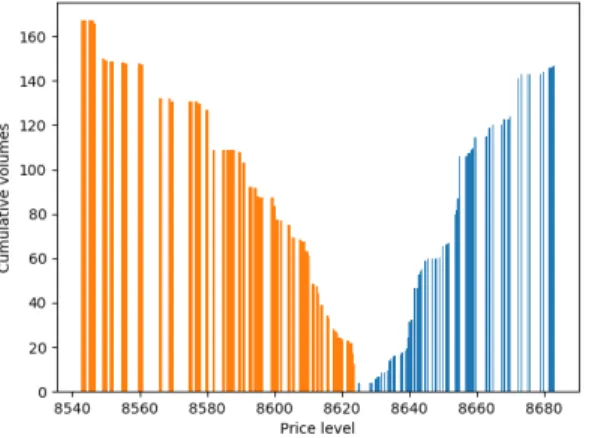
Fig. 1: Example of a limit order book snapshot with depth limited to 100. The asymmetry is due to the higher number of ask orders on the same price levels.
The data is taken from the Coinbase Pro cryptocurrency exchange.
The bid with the largest price at a giventtime:b(t), while the ask with the smallest price at a giventtime:a(t).
Using these notations, the bid-ask spread is defined as
spread=a(t)−b(t) (1)
The middle-price (also referenced as mid-price) is:
a(t)−b(t)
2 (2)
which value is within the spread.
Feature engineering can produce further order book representations that are used as inputs or outputs of machine learning methods. A commonly used repre- sentation is the Volume Weighted Average Price (VWAP). This feature considers not just the price of the orders, but also their side:
Pprice∗volume
Pvolume (3)
It is sometimes considered as a better approximation of the real value of an asset - orders with bigger volume have bigger impact on the calculated price.
A ’snapshot’ of the order book contains the exchange’s orders, ordered by price at a givent time, represented as
adepth, adepth−1, ..., a1, b1, b2, ..., bdepth−1, bdepth (4) , wheredepthis the order book’s depth. In this work we use same depth on both bid and ask sides. A snapshot is visualised in Figure 1. The orders which are closer to the mid-price are more relevant, as these may get executed before other orders which are deeper in the book.
2 Previous works
As the volume of the data increases, data driven machine learning algorithms can exploit deeper context in the larger amount of data. Modeling financial processes has quite a long history, and there already have been many attempts to model markets with machine learning methods. [3] presents one of the most famous models for option pricing, written in 1973, still used today by financial institu- tions. Also, there have been multiple works on limit order books specifically. [4]
examines traders behaviour with respect to the order book size and shape, while e.g [5] is about modelling order books using statistical approaches.
Multiple data sources can be considered for price prediction of financial as- sets. These include, for example LOB data and sentiment of different social media sites, such as Twitter. [6] observes Twitter media to track cryptocurrency news, and also explores machine learning methods to predict the number of fu- ture mentions. [7] targets to use Twitter and Telegram data to identify ’pump and dump’ schemes used by scammers to gain profits.
As limit order books are used in exchanges, many research aim to outperform the market by utilizing LOB data. The most common deep learning models for predicting the price movement are the convolutional neural networks (CNNs) and Long Short-Term Memory (LSTM) networks. [8] emphasizes the time series-like properties of the order book states, and uses specific data preprocessing steps, accordingly.
A benchmark LOB dataset is published [9], however, it is not widely spread yet. It provides normalised time-series data of 10 days from the NASDAQ ex- change, which researchers can use for predicting the future mid-price of the limit order book. The LOBSTER dataset provides data from Nasdaq [10] and is fre- quently used to train data driven models. [11] shows a reinforcement learning based algorithm, which is used for cryptocurrency market making. The authors define 2 types of orders: market and limit, and approach the problem in a market maker’s point of view. They experiment with multiple reward functions, such as
Trade completion or P&L (Profit and Loss). They train deep learning agents using data of the Coinbase cryptocurrency exchange, which is collected through Websocket connection. [12] gives a comprehensive comparison between LSTM, CNN and fully-connected approaches. They have used a wider time-scale, the data are collected from the S&P index between 1950 and 2016.
3 Proposed methods
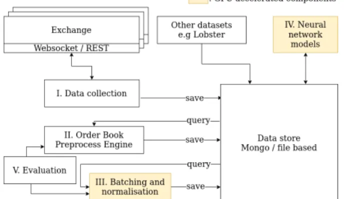
In this section, we introduce the proposed GPU accelerated pipeline for LOB modeling. A high-level overview is shown on Figure 2. The components of the pipeline are executed sequentially. When a computation is done, the result is saved to a centralised database, which is accessable by every component. The next step in the pipeline just grabs the needed data from this data store.
Fig. 2: Block diagram of the proposed GPU accelerated pipeline
The data collection component is used to store the data of the exchange(s) in a database. The Order Book Preprocess Engine is responsible for applying the update messages on a locally maintained LOB, and save snapshots with a fixed time delay between them. Batching and normalisation create normalised data, which is then mapped into discrete intervals and summed up, creating the output. The resulting data can be used as training data for deep neural networks.
The evaluation is the last step of the pipeline, with which the performance of the preprocessing components can be measured. All of the components are detailed in the next sections.
3.1 Data collection
The data format should be universal - no exchange or asset specific features should be included in the process. However, to collect a large enough dataset
for training and performance evaluation, a data collection tool is a part of the pipeline, that can save every update that’s happening on an exchange.
The data collection tool saves the following information from an exchange:
– Snapshot: The tool downloads the current state of the exchange periodically - the length of this period can be supplied when starting the process. The saved data is organised so the snapshots can be queried rapidly by dates.
– Updates: updates that are executed on the exchange and have effect on the order book.
The framework supports multiple assets when (down)loading data, due to the supposed universal features - training with multiple assets may increase the model accuracy [13, 14]. As the number of LOB updates in an exchange can be extremely high, compression is used to store the data.
3.2 Data preparation
The data preparation consists of two steps; the first one is the Order Book Preprocess Engine, which executes specific orders on a locally maintained order book, while the second component is responsible for normalization and batching.
Order Book Preprocess Engine This step applies the LOB updates onto the snapshots, as it would be applied on the exchange itself, thus, creating a time series of LOB snapshots. As this part of the pre-processing purely relies on the previous state of the order book, and needs to be done sequentially, it cannot be efficiently parallelised and transferred to GPUs.
In this paper, only limit orders are considered – market orders are not the scope of the current work, as these are executed instantly. For the Order Book Preprocess Engine, the following order typesare defined that can change the state of the LOB:
– Open: A limit order has been opened by a client.
– Done: A limit order has either been fulfilled or cancelled by the exchange;
it must be removed from the book.
– Match: Two limit orders have been matched, either completely or par- tially. If the match is partial, the volume of the corresponding orders will be changed. If the match is complete, both orders will be removed.
– Change: The client has chosen to change the properties of the order - the price and/or the volume.
There could be additional types of orders on different exchanges, indeed.
The goal of this first phase is to create snapshots of the exchange, by a fixed time gap between them. Each order in the stored book has the following properties:
– Price: The ask or bid price of the order.
– Volume: The volume of the asset which the client would like to sell/buy.
– Id: A unique identifier of the order.
There are only two parameters for this process -time gap between gener- ated snapshotsandLOB depth. We would like to emphasize that this com- ponent does not yet use GPU acceleration, however, it only needs to be run for the whole dataset once. By supplying adequate values for the input parameters - a small enough time frame, and a large enough LOB depth - the normalisation component afterwards can choose to ignore some of the snapshots, or the orders which are too deep in the book.
Batching and normalisation The input of this component is n pieces of snapshots provided by the previous steps. The component can be tore down to smaller pieces - it creates fixed-size or logarithmic intervals, scales the prices of the orders in a snapshot, maps these into the intervals and calculates cumulated sum of the volumes on each side of the LOB. The process is described in details below.
1. Splitting the input data into batches: nconsecutive snapshots are concate- nated (batched) with a rolling window. The number of snapshots in each batch, and the index of the considered snapshots (every 1st, 2nd, 3rd, etc) are parameters. These batches can also be interpreted as matrices, which look like the following:
X1=
a(t−k)d a(t−k)d−1 ... a(t−k)1 b(t−k)1 b(t−k)2 ... b(t−k)d
a(t−k+ 1)da(t−k+ 1)d−1 ... a(t−k+ 1)1 b(t−k+ 1)1b(t−k+ 1)2 ... b(t−k+ 1)d
...
a(t)d a(t)d−1 ... a(t)1 b(t)1 b(t)2 ... b(t)d
(5)
X2=
a(t−k+m)d ... a(t−k+m)1 b(t−k+m)1 ... b(t−k+m)d
a(t−k+m+ 1)d... a(t−k+m+ 1)1b(t−k+m+ 1)1 ... b(t−k+m+ 1)d
...
a(t+m)d ... a(t+m)1 b(t+m)1 b(t+m)2 ... b(t+m)d
(6)
Xl−1=
a(t−k+l∗m)d ... a(t−k+l∗m)1 b(t−k+l∗m)1 ... b(t−k+l∗m)d a(t−k+l∗m+ 1)d ... a(t−k+l∗m+ 1)1b(t−k+l∗m+ 1)1... b(t−k+l∗m+ 1)d
...
a(t+l∗m)d ... a(t+l∗m)1 b(t+l∗m)1 ... b(t+l∗m)d
(7)
In these matrices,tis the timestamp on the last snapshot of the first batch.
d is the order book depth, m shows how many snapshots we skip when generating the next batch, andk is the length of a batch.Xi refers to the actual batch,
2. Normalising each batch independently: the middle price of the last snapshot in the batch is extracted for each, and all the prices in a batch are divided by this value. This also means, for the last snapshot of the batch, the bid prices will always have a value between 0 and 1.0, while the normalised asks will always be larger than 1. However, this limitation does not apply to the previous snapshots of the batch, as the price moves move up or down.
This scaling is necessary, because we intend to use the pipeline for multiple assets. However, one asset could be traded in a price range with magnitudes of difference compared to other assets. Applying the proposed normalisation
causes prices of any asset to be scaled close to 1. This will make the input for the neural network model quasi standardised.
3. Determining price levels for the 0-th order interpolation. In this step, the discrete values are calculated, which will be used for representing an interval of prices levels in the order book. These will contain the sum of volumes available in each price range at the end of processing.
The pipeline offers two methods to create these: linear (the intervals has the same size) and logarithmic (the intervals closer to the mid-price are smaller).
The logarithmic intervals have a benefit over the linear ones: choosing linear intervals that are nor too big or too small needs optimization, as there could be larger price jumps - considering volatile assets and periods. These jumps could cause the values to be outside the intervals. With logarithmic intervals, this problem can be decreased, as the intervals on both sides can collect a much greater range of price values. Furthermore, prices around the spread are the most important ones, as discussed above – which are represented more detailed in the logarmithmic case.
One interval can be notated as:
[rlower;rupper) (8)
wherelowerandupperare the limits. In this step, multiple of these intervals are created, and stored in a list:
[r1;lower;r1;upper),[r2;lower;r2;upper), ...[rn;lower, rn;upper) (9) The lower bound of thek+ 1th interval always equals to the upper bound of thekth interval.
The selected intervals are re-used through the application, in the next steps.
4. 0-th order interpolation and summation. For each order in a snapshot the corresponding interval is defined (the price of the order is between the limits of the interval). This is done by iterating over the intervals, and verifying the price of the orders:
ri;lower≤price < ri,upper (10) where i is the index of the actual interval. The volumes of orders which should be put into the same interval are summed. At the end of this step, the output contains the sum of volumes for each interval.
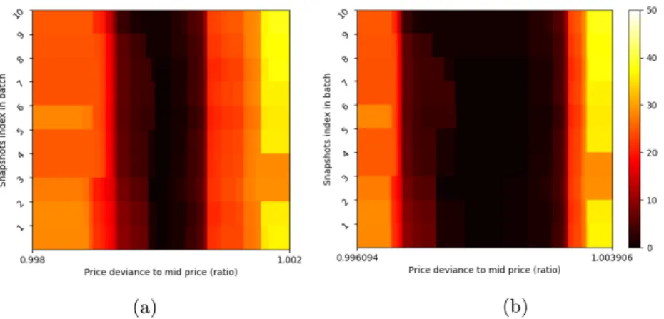
5. Iterating through the intervals which contain the volumes and calculating the accumulated volumes, separately for bid and ask side. At the beginning of this step, the summed volume for each interval is known. After the step is done, the value in each interval tells what is the volume that can be bought/sold below/above the lower/upper price level of the interval. When this part of the processing is done, the output for each snapshot could be plotted as in Figure 1. This step can also be parallelized for each batch. An example to a completely processed batch can be seen on Figure 3a and 3b.
(a) (b)
Fig. 3: An example of the preprocessed LOB batch of 200 intervals with 30 depth.
3a was generated with linear scaling, while 3b uses logarithmic scale. Data taken from Coinbase Pro, 29. 10. 2019
6. Generating labels for the batches. This step is required for supervised learn- ing algorithms to define a target variable for every batch. In the scope of this work, the mid-price and VWAP properties of the order book have been cho- sen to be used as labels, however, it can be arbitrary. Labels are generated according to the snapshots after the batch and scaled by the mid-price (or VWAP) of the last snapshot in the batch. If a regression model is used, then the value itself is the target variable. If the goal is to have a classification model, the target value can be clustered e.g., into 3 labels:
– Upward, downward and sliding movement. When calculating these, an α parameter is considered, which is a percentage value. If the average of the next snapshots is greater than (1 +α)∗midpriceit is considered upward. If it is less than (1 +α)∗midpriceit is downward, else the batch is labelled as a sideway movement.
The steps above result in a set of batches, where each batch containsnsnap- shots and corresponding output label(s). When displaying a batch, the relative price movement over time can be discovered.
4 Evaluation and Results
In order to measure the speed enhancements of the proposed methods, experi- ments with different data sizes and hardware accelerators have been carried out.
The evaluation was done with data taken with the data collection tool. The data was collected with Coinbase Pro API. Coinbase exchange provides REST support for polling snapshots. For evaluation, a snapshot has been saved each 5 minutes, while the updates of the book are provided via Websocket streams.
4.1 Used data
The data used for performance measurement was collected from the Coinbase exchange, using 4 currency pairs - BTC-USD, BTC-EUR, ETH-USD, XRP- USD, starting in September, 2019. For the test, we have limited the number of updates processed - the algorithm would stop after the supplied ‘n’ number of updates - ‘n’ is shown in Table 1. As the data contains discrepancies due to the Websocket connection, this does not mean that the number of processed snapshots and updates will always translate to the same number of batches - hence the number of batches slightly vary across the measurements - e.g 2088 batches were generated for 100000 updates, but only 9941 for 1 million updates.
The reason why we did not consider batches as the base limitation, is that in real-life scenarios these discrepancies would also happen.
4.2 Hardware and software architecture
The GPU accelerated pipeline extensively uses the Numpy and Numba packages - the CUDA accelerated code was written using Numba’s CUDA support. To compare the performance the pipeline was executed on different GPUs (single GPU in each run) for the same amount of raw data. The deep learning models were created with Keras. The data collection, preparation and trainings were run in a containerized environment, using Docker.
The hardware units used in the tests:
– GPU 1: NVidia Titan V, 5120 CUDA cores, 12 GB memory.
– GPU 2: NVidia Titan Xp, 3840 CUDA cores, 12 GB memory.
– GPU 3: NVidia Titan X, 3072 CUDA cores, 12GB DDR5 memory.
– CPU: Intel Core i7-6850K CPU, 3.60GHz
4.3 Execution time
In the first phase of the pipeline – the Order Book Preprocess Engine – the updates are sequential, which makes its execution in parallel a difficult problem.
Because of that, the measurements have been broken into 2 parts: the snapshot generation and the parallellised normalisation with other steps.
Table 1 shows the measurements taken on the Preproces Engine component, while Table 2 measures the components that apply the normalisation on the output of the Preprocess Engine. For comparison, the CPU column runs the same algorithms, but using plain Python with libraries such as Numpy. In the
’CPU + LLVM’ measurements, we utilise the optimization techniques of the Numba library. This project uses a just-in-time compiler to compile certain steps of the process - the same steps which are accelerated by CUDA when running on a GPU. We have chosen the CPU + LLVM method as a comparison base - the GPU performance is compared to this one. Some experiments were made on using parallel execution models of the Numba library (such as prange) - which did not bring significant performance improvements. Also, it’s worth to note,
that a server-grade CPU, which uses many more cores compared to the used one could speed up the results when executing parallelly.
Table 1: Performance of the Order Book Preprocess Engine component. Data taken from the Coinbase Exchange. The time delay between the snapshots is 1 second.
Pipeline performance Batches generated Time taken [sec-
onds)]
Nr. of processed updates
2088 8.4 seconds 100000
9941 18.4 seconds 1000000
90086 169.58 seconds 10000000
504880 792.01 seconds 57.35 million
Table 2: Performance measurements of preparing the data after the Order Book Preprocess Engine. (LOB depth: 100, batch size: 10).
Pipeline performance [seconds]
Data used CPU CPU + LLVM GPU 1 GPU 2 GPU 3
2070 batches 129.93 2.08 2 1.7 1.71
9941 batches 641.84 3.9 2.59 2.6 3.2
504880 batches 19404.38 137.237 58.76 61.77 101,86
4.4 Inference
To be able to integrate the solution into real-world trading environment, the pipeline should be able to process the stream of order book data and execute the steps even for a single batch as fast as possible. To simulate the inference phase time measurements were carried out with only a few snapshots. In these experiments 500 updates were used, from which 29 snapshots were created. The first phase - applying these updates and creating the next snapshots - took 7 seconds to generate 29 snapshots (0.15 seconds / snapshot). Normalising with CPU took 2.06 seconds (0.071 seconds / snapshot), while it took around 1.70, 1.95, 1.59 on the Titan V/Xp/X GPUs. The processing took 0.058/0.067/0.054 seconds / snapshot on each of them. This means there is is 18% improvement when running on Titan V, and 22% on the Titan X).
5 Application and conclusions
The most important feature of the GPU accelerated pipeline is that with the performance gain multiple parameter setups can be tested in less time, when compared with CPU preprocessing. The solution helps researchers to train deep learning models with several kinds of data representation and labelling meth- ods and parameters - and select the method which yields the best accuracy.
In absance of a GPU, the LLVM compiler can also improve on processing the data. The proposed GPU accelerated pipeline uses structured input data in a
way that’s not specific to any data source. As a result, it could be used for any exchange, which provides an interface to their order book data. Financial in- stitutions or individual clients on the exchange could benefit from the proposed pipeline, as it helps them make data processing and normalisation much faster by running on the GPU instead of a CPU. An additional benefit of the pipeline is its modularity - the components can be used independently of each other. In future research, the pipeline can be performance-tested with multiple hyperparameter set-ups, and the GPU execution can be further investigated using profilers. The pipeline can also be the base of a real-time, GPU accelerated trading bot.
The solution is available at https://github.com/jazzisnice/LOBpipeline.
References
1. Kuzman Ganchev, Michael Kearns, Yuriy Nevmyvaka, and Jennifer Wortman Vaughan. Censored exploration and the dark pool problem, 2012.
2. Yann LeCun, Yoshua Bengio, and Geoffrey Hinton. Deep learning. nature, 521(7553):436–444, 2015.
3. Fischer Black and Myron Scholes. The pricing of options and corporate liabilities.
Journal of Political Economy, 81(3):637–654, 1973.
4. Angelo Ranaldo. Order aggressiveness in limit order book markets. Journal of Financial Markets, 7:53–74, 01 2004.
5. Rama Cont, Sasha Stoikov, and Rishi Talreja. A stochastic model for order book dynamics. Operations Research, 58:549–563, 06 2010.
6. Johannes Beck, Roberta Huang, David Lindner, Tian Guo, Zhang Ce, Dirk Hel- bing, and Nino Antulov-Fantulin. Sensing social media signals for cryptocurrency news. Companion Proceedings of The 2019 World Wide Web Conference on - WWW ’19, 2019.
7. Mehrnoosh Mirtaheri, Sami Abu-El-Haija, Fred Morstatter, Greg Ver Steeg, and Aram Galstyan. Identifying and analyzing cryptocurrency manipulations in social media, 2019.
8. Avraam Tsantekidis, Nikolaos Passalis, Anastasios Tefas, Juho Kanniainen, Mon- cef Gabbouj, and Alexandros Iosifidis. Using deep learning for price prediction by exploiting stationary limit order book features, 2018.
9. Adamantios Ntakaris, Martin Magris, Juho Kanniainen, Moncef Gabbouj, and Alexandros Iosifidis. Benchmark dataset for mid-price forecasting of limit order book data with machine learning methods. Journal of Forecasting, 37(8):852–866, Aug 2018.
10. Markus Bibinger, Christopher Neely, and Lars Winkelmann. Estimation of the dis- continuous leverage effect: Evidence from the nasdaq order book. Federal Reserve Bank of St. Louis, Working Papers, 2017, 04 2017.
11. Haoran Wei, Yuanbo Wang, Lidia Mangu, and Keith Decker. Model-based rein- forcement learning for predictions and control for limit order books, 2019.
12. Luca Di Persio and O. Honchar. Artificial neural networks architectures for stock price prediction: Comparisons and applications. 10:403–413, 01 2016.
13. Justin Sirignano and Rama Cont. Universal features of price formation in financial markets: perspectives from deep learning, 2018.
14. Zihao Zhang, Stefan Zohren, and Stephen Roberts. Deeplob: Deep convolutional neural networks for limit order books. IEEE Transactions on Signal Processing, 67(11):3001–3012, Jun 2019.