DOI: 10.1556/606.2020.15.2.3 Vol. 15, No. 2, pp. 25–36 (2020) www.akademiai.com
GRAPH APPROXIMATION ON SIMILARITY BASED ROUGH SETS
1 Dávid NAGY*, 2 Tamás MIHÁLYDEÁK, 3 László ASZALÓS
Department of. Computer Science, Faculty of Informatics, University of Debrecen e-mail: 1nagy.david@inf.unideb.hu, 2mihalydeak.tamas@inf.unideb.hu
3aszalos.laszlo@inf.unideb.hu
Received 1 January 2019; accepted 21 November 2019
Abstract: Correlation clustering is a widely used technique in data mining. The clusters contain objects, which are typically similar to one another and different from objects from other groups. In the authors previous works the possible usage of correlation in rough set theory were investigated. In rough set theory, two objects are treated as indiscernible if all of their attribute values are the same. A base set contains those objects that are indiscernible from one another. The partition, gained from the correlation clustering, can be understood as the system of base sets, as the clusters contain the typically similar objects (not just to a distinguished member) and it considers the real similarity among the objects. In this work the extension of this study is presented, using the method to approximate graphs representing similarity relations.
Keywords: Correlation clustering, Rough set theory, Graph approximation
1. Rough set theory
In the classic sense, a set contains some objects that share a common property. If the question is whether an object is in the set or not, then the answer is yes or no. For instance, in case of the set of prime numbers 2 is in the set but 4 is not. However, in many applications there some sets where answering the previous question is not that simple. An appropriate example is the set of brave warriors. Bravery is a concept, where it is difficult to decide whether a warrior can belong to this set or not, because somebody can treat a person as brave, but another person can treat this warrior as not
*
brave. These kinds of concepts are called vague. Rough set theory was proposed by Zdzisław Pawlak [1]-[3]. The main goal of this theory is to handle vague concepts based on some background knowledge.
In many real world applications objects are stored in datasets or databases. Datasets can be given by an information system, which is a pair ISA = (U,A), where U is a set of objects called the universe and A is a set of attributes. Let : → be a function, where Va denotes the domain of attribute a. An information system can be represented by a table, where each row is an entity of the universe, and the columns represent the attributes. Any pair (x,a), where ∈ and ∈ in the table is a cell whose value is a(x).
In this system two objects can be truly distinguished, if they differ in at least one of attribute value. In a Pawlakian system two objects are called indiscernible, based on some background knowledge, if they have the same attribute values. This indiscernibility relation is an equivalence relation, and it can be defined in the following way:
Let ′⊆ be a set of attributes, , ∈ be two arbitrary objects;
if and only if = for every ∈ ′, (1)
where R is called the indiscernibility relation. The background knowledge can come from an information system or a database.
The R relation defines a partition based on a set of attributes A’. The members of this partition are called base sets and they are the granules of knowledge.
Mathematically, the system of base sets can be defined in the following way:
= | ⊆ and , ∈ if . (2)
Indiscernibility plays a very important role in decision making. If a decision about an object needs to be stated, then the same decision must be made about those members that are indiscernible from this object. As mentioned earlier in classical set theory, there exist only two answers to the question, whether an object is in the set or not. In rough set theory the number of possible answers is 3. Let S be a set and ∈ an object,
• It is sure that ∈ ! if ∀ : ∈ and then ∈ !,
• It is possible that ∈ ! if ∃ : ∈ and then ∈ !, (3)
• It is sure that ∉ ! if ∀ : ∈ and then ∉ !.
A vague set can be represented by two sets. This process is called the approximation of a set. For any vague set S the following two sets can be given:
% ! = ⋃ | ∈ and ⊆ ! , (4)
' ! = ⋃ | ∈ and ∩ ! ≠ ∅ , (5)
where l(S) is called the lower approximation which contains those objects that surely belong to the set; and u(S) is the upper approximation of the set S which is the collection of those members that possibly belong to S.
The set BN(S) is called the boundary region and can be defined by the following formula:
/ ! = ' 0 \% ! . (6)
If the boundary region is empty, then the set is crisp, otherwise it is rough. A rough set can also be characterized numerically by the following coefficient:
23=|' ! ||% 0 |. (7)
It is called the accuracy of the approximation. Naturally 0 ≤ 67≤ 1 and its value is 1 if the set is crisp. In the formula |!| denotes the cardinality of a finite set.
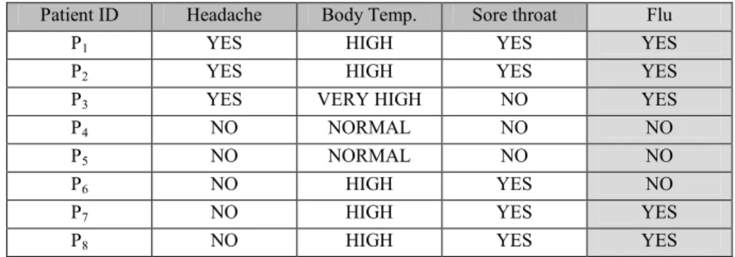
Table I shows a very simple table containing 8 rows. Each of them represents a patient and each has 3 attributes: headache, body temperature, and the presence of a sore throat. The first column is only used for identifying the patients. The goal is to determine whether a person has the flu or not based on the previously mentioned three attributes. It can be seen that there are some inconsistency, as patient P6 and P7 have the same attribute values and P6 does not have the flu, but P7 does. Rough set theory is a possible tool for handling this kind of inconsistency.
Table I
Information System
Patient ID Headache Body Temp. Sore throat Flu
P1 YES HIGH YES YES
P2 YES HIGH YES YES
P3 YES VERY HIGH NO YES
P4 NO NORMAL NO NO
P5 NO NORMAL NO NO
P6 NO HIGH YES NO
P7 NO HIGH YES YES
P8 NO HIGH YES YES
The base sets (based on the attributes {Headache, Body Temp, Sore Throat}) contain patients with the same symptoms and it is the following:
= : ;<, ;= , ;> , ;?, ;@ , ;A, ;B, ;C D. (8) Let S be the set of those patients who have the flu:
! = ;<, ;=, ;>, ;B, ;C . (9) The approximation of the set can be given by its lower and upper approximation:
% ! = ;<, ;=, ;> , (10)
' ! = ;<, ;=, ;>, ;A, ;B, ;C . (11) The accuracy of the approximation is 0.5.
2. Correlation clustering
Clustering is a widely used tool of unsupervised learning. Its task is to group objects in a way, that the objects in one group (cluster) are similar, and the objects from different groups are dissimilar. This defines an equivalence relation. The similarity is usually based on the distance of the objects. However, sometimes only categorical data are given where distance is meaningless. For example: what is the distance between a man and a woman? In this case a tolerance relation is needed. Two objects can be treated as similar if this relation holds for these two objects. If the relation does not hold for two objects, then they are dissimilar. Naturally, this relation is reflexive, because every object is similar to itself. It is also symmetric, which can be easy to see. The transitivity, however, does not necessarily hold. Correlation clustering is a clustering technique, which is based on a tolerance relation [4]-[6]. The goal of correlation clustering is to find an equivalence relation, which is closest to the similarity (tolerance) relation. Let V be a set of objects and E ⊂ × the tolerance relation. The result of correlation clustering is partition. This partition can be defined as a function:
I = → 1, ⋯ , K . So it assigns for each object an integer number, which is its cluster IDentification number (ID). The objects A and B are in the same group if I = I .
The following two cases can be treated as conflicts for two arbitrary objects A and B:
E holds, but I ≠ I ,
E does not hold, but I = I . (12)
The cost function f is the number of these disagreements. The value of the function f is the distance between the tolerance relation T and the equivalence relation defined by the partition. Solving a correlation clustering problem is equivalent to minimizing its cost function. The partition is called perfect if the cost function value is 0. It is easy to show that for an arbitrary tolerance relation, there is no necessarily perfect partition.
Correlation clustering has many applications: image segmentation [7]; identification of biologically relevant groups of genes [8]; examination of social coalitions [9];
reduction of energy consumption [10]; modeling physical processes [11]; (soft) classification [12], [13], etc.
Despite its many applications, it has a disadvantage. It is a Nondeterministic Polynomial (NP) time complete problem, so it is very complicated to find the partition with minimal cost function value. The number of partitions also grows exponentially. It can be given by the Bell number [14]. In general - even in the case of some dozens of objects - the optimal partition cannot be determined in reasonable time. However, a quasi-optimal solution can be enough in practical cases. This can be achieved by using search algorithms.
3. Similarity based rough sets
As mentioned earlier, the Pawlakian indiscernibility relation is an equivalence relation, which can be too strict in many applications. Sometimes a similarity relation, which can be represented by a tolerance relation, is enough. In the literature there are some research projects that try to generalize the classical rough set theory. One possible way is the so-called covering systems [15].
These systems generalize the Pawlakian systems in two way:
1. The R indiscernibility relation is replaced by a tolerance relation (similarity relation);
2. = NOP | ∈ and ∈ N P if U where | ∈ and .
In a Pawlakian system a base set contains objects that are indiscernible from one another, while in a covering system it contains objects that are similar to a distinguished member (in the above formula it is the x member). So two entities are considered as similar because they are similar to a third distinguished one. These systems can handle the fact that the indiscernibility relation is weakened to a tolerance relation, but it also has some issues. The main problem is that it does not consider the real similarity among objects but the similarity to special member. The number of base sets can be also high.
In the worst case, its value is the number of objects.
Correlation clustering defines a partition. The clusters contain objects that are typically similar to one another. In the authors’ previous works [16], [17], it was shown that this partition can be understood as the system of base sets. The approximation space given this way has several good properties. The most important one is that it focuses on the similarity (the tolerance relation) itself, and it is different from the covering type approximation space relying on the tolerance relation. The system of base sets can be defined by the following way, where p denoted the partition gained from the correlation clustering:
= | ⊆ and , ∈ if I = I U . (13)
Singleton clusters represent very little information, because the system could not consider its member similar to any other objects without increasing the number of conflicts. As they mean little information, they can be left out. If the singleton clusters are not considered, then a partial system of base sets can be generated from this partition where singleton clusters are not base sets.
4. Graph approximation
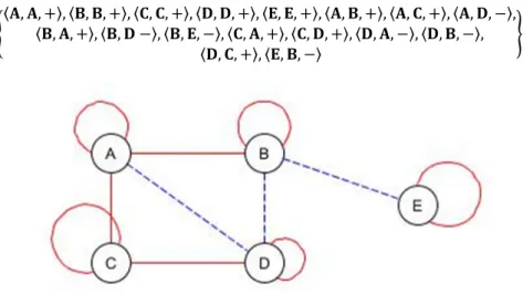
A similarity relation can be represented by a signed graph. This graph [18], [19] is complete if the relation is total, and it is not complete if the relation is partial. Because of the symmetry, it must be an undirected graph. Due to the reflexivity every vertex in the graph has a self-loop edge. If two objects are similar, then a positive edge runs between them, and if they are different, then the edge is negative. Every graph can be represented by a set that contains ordered pairs. In this case, it can be represented by a set of 3-tuples.
The graph in Fig. 1 can be represented by the following set:
[\ , , ]^, \ , , ]^, \_, _, ]^, \`, `, ]^, \a, a, ]^, \ , , ]^, \ , _, ]^, \ , `, b^,
\ , , ]^, \ , ` b^, \ , a, b^, \_, , ]^, \_, `, ]^, \`, , b^, \`, , b^, \`, _, ]^, \a, , b^ c.
Fig. 1. A similarity relation represented by a signed graph
The main goal of this paper is extending the principles of similarity based rough sets to graphs that represent similarity relations. From the theoretical point of view, a Pawlakian approximation space can be characterized by an ordered pair \ , ^, where U denotes the universe (a nonempty set of objects) and R denotes the indiscernibility relation. In similarity based rough sets, R is a similarity relation (tolerance relation).
In case of graph approximation, the universe is a complete undirected signed graph in which every node is connected to every node by 2 edges (one positive and one negative) and every node has also 2 self-loop edges. Formally d = × × ], b .
Let d<⊂ d be graph representing an arbitrary similarity relation. This graph defines the background knowledge. The R relation is also defined by this e< graph. For all objects , ∈ if , , ] ∈ d< then the objects are similar and if , , b ∈ d< then they are different.
In rough set theory (and also in its similarity based version), the base sets provides the knowledge about the system. Here there are base graphs, and they represent the same. The system of base graphs is also determined by the correlation clustering, and it can be given by the following formula:
= : | ⊆ df and \ , , g^ ∈ if I = I and g ∈ ], b D. (14) Let d=⊂ d< be an arbitrary subgraph of d<. The lower and upper approximation of d= can be given by the following way:
% d= =∪ | ⊆ and ⊆ d= , (15)
' d= =∪ | ⊆ and ∩ d=≠ 0 . (16)
The lower approximation is the disjoint union of those base graphs that are subgraphs of d=. The upper approximation is the disjoint union of those base graphs for which there exist a graph which is a subgraph of both d< and d=.
The accuracy of the approximation can be calculated by the following fraction, where N(G) denotes the number of self-loop edges in a graph:
6jk=|' d|% dkk| =| =⁄ m/n% d⁄ m/n' dokpp (17)
Graph approximation uses the same concepts as the set approximation. However, it is a stricter method, as it takes into consideration not only the objects but the edges too.
5. Attribute reduction with graph approximation
In data mining a natural question can be if some data can be removed from the system preserving its basic properties (whether a table contains some superfluous data).
In this paper a method is proposed to measure the dependency between two attributes (or set of attributes). If this dependency value is above a threshold, then one of the attributes can be removed.
Let q! = , an information system and ′, ′′ ⊂ two sets of attributes. Let d<
be the graph representing the similarity relation, which is based on the attribute set ′. Let d= be the graph representing the similarity relation which is based on the attribute set ′′. To measure the dependency between ′ and ′′ the following method is proposed:
1. Determine the system of base graphs based on e<;
2. Approximate d= using the base graphs defined in the first step;
3. Calculate the accuracy of approximation;
4. If the accuracy is higher than a threshold, then ′′ can be treated as superfluous.
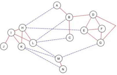
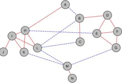
In the following figures, a very simple example is shown with 14 objects. In Fig. 2 a graph can be seen, which denotes a similarity based on a set of attributes. In the figure the solid lines denote the similarity, while the dashed ones denote the difference between objects.
Fig. 2. G1 graph representing a similarity relation based on a set of attributes
In Fig. 3 the base graphs can be observed which were generated by the correlation clustering. In this example there are three base graphs.
Fig. 3. The base graphs generated by the correlation clustering
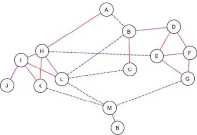
Fig. 4 shows another graph, which also illustrates another set of attributes. It is important that the similarity is based on the same objects as before. The difference between d< and d= is negligible. It can be observed only in 4 edges. Between objects A and H the negative edge was replaced by a positive one. Between objects K and N the edge was deleted as well as between D and G. Between A and B the positive edge was changed to negative.
In Fig. 5 the lower approximation and in Fig. 6 the upper approximation can be seen. It is interesting that even though there are only slight differences between the two
graphs the lower approximation contains only the two smallest base graphs. The reason is that graph approximation is stricter, because it takes into consideration the edges. As objects A and B became different, the base graph containing them cannot be in the lower approximation, only in the upper approximation.
Fig. 4. G2 graph representing a similarity relation based on a set of attributes with the same objects
Fig. 5. The lower approximation of G2
Fig. 6. The upper approximation of G2
The accuracy of the approximation is:
uvk =<?=w~0.48.
This means that based on G1 the percentage of the available information about G2 is only 48% even though they are almost equivalent. This method takes into account the real similarity among objects; therefore it can give appropriate results in situations, where other algorithms proved to be a dead end. For example, in mathematical statistics a common method to measure the dependency between attributes is correlation.
Although, it works only if there is a linear relationship between the attributes. The method of this paper can work in various applications for any types of relationships.
6. Conclusion
Rough set theory offers a way to handle vague concepts. In its classical variant, two objects are considered as indiscernible if all of their known attribute values (based on background knowledge) are the same. The base sets contain entities that are indiscernible from one another and they represent the granules of knowledge and also the limit of the background knowledge.
Correlation clustering is a clustering technique, which is based on a similarity relation. Its result is a partition, and the clusters contain objects that are typically similar to one another. This property is very important because this partition can be understood as the system of base sets. Thus, a new approximation space appears. In this paper a possible method was shown to handle the approximation of graph representing similarity relations. Graph approximations can be a way to reduce attributes that are
superfluous. As a future plan, it could be very interesting to use the method described in the paper on real data.
Acknowledgements
This work was supported by the construction EFOP-3.6.3-VEKOP-16-2017-00002.
The project was supported by the European Union, co-financed by the European Social Fund.
Open Access statement
This is an open-access article distributed under the terms of the Creative Commons Attribution 4.0 International License (https://creativecommons.org/licenses/by/4.0/), which permits unrestricted use, distribution, and reproduction in any medium, provided the original author and source are credited, a link to the CC License is provided, and changes - if any - are indicated. (SID_1)
References
[1] Pawlak Z. Rough sets, International Journal of Computer & Information Sciences, Vol. 11, No. 5, 1982, pp. 341–356.
[2] Pawlak Z. Rough sets, Theoretical aspects of reasoning about data, Kluwer, 1991.
[3] Pawlak Z., Skowron A. Rudiments of rough sets, Information Sciences, Vol. 177, No. 1, 2007, pp. 3–27.
[4] Bansal N., Blum A., Chawla S. Correlation clustering, Machine Learning, Vol. 56, No. 1-3, 2004, pp. 89–113.
[5] Becker H. A survey of correlation clustering, COMS E6998: Advanced Topics in Computational Learning Theory, 2005.
[6] Zimek A. Correlation clustering, ACM SIGKDD Explorations Newsletter, Vol. 11, No. 1, 2009, pp. 53–54.
[7] Kim S., Nowozin S., Kohli P., Yoo C. D. Higher-order correlation clustering for image segmentation, Advances in Neural Information Processing Systems, Vol. 24, 2011, pp. 1530–1538.
[8] Bhattacharya A., De R. K. Divisive correlation clustering algorithm (dcca) for grouping of genes: detecting varying patterns in expression profiles, Bioinformatics, Vol. 24, No. 11, 2008, pp. 1359–1366.
[9] Yang B., Cheung W. K., Liu J. Community mining from signed social networks, IEEE Transactions on Knowledge and Data Engineering, Vol. 19, No. 10, 2007, pp. 1333–1348.
[10] Chen Z., Yang S., Li L., Xie Z. A clustering approximation mechanism based on data spatial correlation in wireless sensor networks, IEEE Wireless Telecommunications Symposium, Tampa, FL, USA, 21-23 April 2010, pages 7.
[11] Neda Z., Florian R., Ravasz M., Libál A., Györgyi G. Phase transition in an optimal clusterization model, Physica A, Statistical Mechanics and its Applications, Vol. 362, No. 2, 2006, pp. 357–368.
[12] Aszalos L., Mihálydeák T. Rough clustering generated by correlation clustering, In: Ciucci D., Inuiguchi M., Yao Y., Ślęzak D., Wang G. (Eds) Rough Sets, Fuzzy Sets, Data Mining,
and Granular Computing, Lecture Notes in Computer Science, Vol. 8170, Springer, Berlin, Heidelberg 2013, pp. 315–324.
[13] Aszalos L., Mihálydeák T. Rough classification based on correlation clustering, in: Miao D., Pedrycz W., Ślȩzak D., Peters G., Hu Q., Wang R. (Eds) Rough Sets and Knowledge Technology, Lecture Notes in Computer Science, Vol. 8818, Springer, 2014, pp. 399–410.
[14] Aigner M. Enumeration via ballot numbers, Discrete Mathematics, Vol. 308, No. 12, 2008, pp. 2544‒2563.
[15] Yao Y., Yao B. Covering based rough set approximations, Information Sciences, Vol. 200, 2012, pp. 91–107.
[16] Nagy D., Mihálydeák T., Aszalós L. Similarity based rough sets, in: Polkowski L., Yao Y., Artiemjew P., Ciucci D., Liu D., Ślęzak D., Zielosko B. (Eds) Rough Sets, Lecture Notes in Computer Science, Springer, Vol. 10314, 2017, pp. 94–107.
[17] Nagy D., Mihálydeák T., Aszalós L. Similarity based rough sets with annotation, in:
Nguyen H., Ha Q. T., Li T., Przybyła-Kasperek M. (Eds) Rough Sets, Lecture Notes in Computer Science, Springer, Vol. 11103, 2018, pp. 88‒100.
[18] Szabó S. Conflict graphs in implicit enumeration, Pollack Periodica, Vol. 7, No. Suppl. 1, 2012, pp. 145‒156.
[19] Etlinger J., Rák O., Zagorácz M., Máder P. M. Revit add-on modification with simple graphical parameters, Pollack Periodica, Vol. 13, No. 3, 2018, pp. 73‒81.