V L F L M H G D T B TheForcedResponseoftheElNi ñ o–SouthernOscillation–IndianMonsoonTeleconnectioninEnsemblesofEarthSystemModels 2163

(1)

The Forced Response of the El Niño–Southern Oscillation–Indian Monsoon Teleconnection in Ensembles of Earth System Models

TAMÁSBÓDAI

Pusan National University, and Center for Climate Physics, Institute for Basic Science, Busan, South Korea, and Department of Mathematics and Statistics, and Centre for the Mathematics of the Planet Earth, University

of Reading, Reading, United Kingdom

G_ÁBORDRÓTOS

Instituto de Fı´sica Interdisciplinar y Sistemas Complejos, CSIC-UIB, Palma de Mallorca, Spain, and MTA–ELTE Theoretical Physics Research Group, and Institute for Theoretical Physics, Eotv€ os University, Budapest,€

Hungary, and Max-Planck-Institut fur Meteorologie, Hamburg, Germany€

MÁTYÁSHEREIN

MTA–ELTE Theoretical Physics Research Group, and Institute for Theoretical Physics, Eotv€ os University,€ Budapest, Hungary, and CEN, Meteorological Institute, University of Hamburg, Hamburg, Germany

FRANKLUNKEIT

CEN, Meteorological Institute, University of Hamburg, Hamburg, Germany

VALERIOLUCARINI

Department of Mathematics and Statistics, and Centre for the Mathematics of the Planet Earth, University of Reading, Reading, United Kingdom, and CEN, Meteorological Institute, University of Hamburg, Hamburg, Germany, and Walker Institute for Climate System Research, University of Reading, Reading, United Kingdom

(Manuscript received 11 May 2019, in final form 19 November 2019) ABSTRACT

We study the teleconnection between El Niño–Southern Oscillation (ENSO) and the Indian summer monsoon (IM) in large ensemble simulations, the Max Planck Institute Earth System Model (MPI-ESM), and the Community Earth System Model (CESM1). We characterize ENSO by the June–August Niño-3 box-average SST and the IM by the June–September average precipitation over India, and define their teleconnection in a changing climate as an ensemble-wise correlation. To test robustness, we also consider somewhat different variables that can characterize ENSO and the IM. We utilize ensembles converged to the system’s snapshot attractor for analyzing possiblechanges in the teleconnection. Our main finding is that the teleconnection strength is typically increasing on the long term in view of appropriately revised ensemble-wise indices. Indices involving a more western part of the Pacific reveal, furthermore, a short-term but rather strong increase in strength followed by some decrease at the turn of the century.

Using the station-based Southern Oscillation index (SOI) as opposed to area-based indices leads to the identification of somewhat more erratic trends, but the turn-of-the-century ‘‘bump’’ is well detectable with it. All this is in contrast, if not in contradiction, to the discussion in the literature of a weakening teleconnection in the late twentieth century.

We show here that this discrepancy can be due to any of three reasons: 1) ensemble-wise and temporal correlation coefficients used in the literature are different quantities; 2) the temporal moving correlation has a high statistical variability but possibly also persistence; or 3) MPI-ESM does not represent the Earth system faithfully.

Denotes content that is immediately available upon publication as open access.

Supplemental information related to this paper is available at the Journals Online website:https://doi.org/10.1175/JCLI-D-19-0341.s1.

Corresponding author: Mátyás Herein, hereinm@gmail.com DOI: 10.1175/JCLI-D-19-0341.1

Ó2020 American Meteorological Society. For information regarding reuse of this content and general copyright information, consult theAMS Copyright Policy(www.ametsoc.org/PUBSReuseLicenses).

Downloaded from http://journals.ametsoc.org/jcli/article-pdf/33/6/2163/4954840/jclid190341.pdf by guest on 31 July 2020

(2)

1. Introduction

Probably the most important teleconnection phe- nomena are those of El Niño–Southern Oscillation (ENSO) (Trenberth 1976;Trenberth 1984;Bjerknes 1969;

Neelin et al. 1998). ENSO is a natural, irregular fluctuation phenomenon in the tropical Pacific region (Timmermann et al. 2018) and mostly affects the tropical and the sub- tropical regions; however, it has an impact on the global climate system as well. A crucial and open question that has challenged scientists for decades is how ENSO would change as a result of the increasing radiative forcing due to the increasing greenhouse gas concentrations. The IPCC has low confidence in what would exactly happen to ENSO in the future, even though they have high confidence that ENSO itself would continue (Christensen et al.

2013). There have been several studies (e.g., Guilyardi et al. 2009;Collins et al. 2010; Vecchi and Wittenberg 2010;Cai et al. 2015) that aimed to reveal how ENSO might respond to greenhouse-gas forcing. However, most of the applied methods have a common drawback: they evaluate averages and further statistical quantifiers (in- cluding variances, correlations, etc.) with respect to time in a time-dependent dynamical system (i.e., in our changing climate or in simplified models thereof).

In a changing climate, where one or more relevant pa- rameters are changing in time, there can be no stationarity by definition, whereas stationarity is crucial for the applicability of temporal averages, as illustrated byDrótos et al. (2015) in a toy model. In realistic GCMs globally averaged quantities seem to behave better, but the problem proves to be significant for local quantities and teleconnections (Herein et al. 2016;Herein et al. 2017). Since the ENSO events are identified by temperatures that are warmer or cooler than average, and teleconnections are defined as correlations between such anomalies, it is important to have a firmly established notion of averages when climatic means are shifting, as also pointed out by L’Heureux et al. (2013,2017)andLindsey (2013).

To properly address the problem of evaluating averages in a changing climate, in this study we turn to a gradually strengthening view according to which the relevant quantities of the climate system are the statistics taken over an ensemble of possible realizations evolved from various initial conditions (see, e.g.,Bódai et al. 2011;Bódai and Tél 2012;Deser et al. 2012;Daron and Stainforth 2015; Kay et al. 2015; Stevens 2015;

Bittner et al. 2016;Herein et al. 2016;Herein et al. 2017;

Drótos et al. 2017;Hedemann et al. 2017;Lucarini et al.

2017;Suárez-Gutiérrez et al. 2017;Li and Ilyina 2018;

Maher et al. 2019). We can trace back this view toLeith (1978), which was recently revived (Branstator and Teng 2010) and rediscovered independently also by others. In

contrast to weather forecasting, one focuses here on long-term properties, independent of initial conditions, in order to characterize the internal variability, as well as the forced response of the climate. The mathematical concept that provides an appropriate framework is that of snapshot (Romeiras et al. 1990;Drótos et al. 2015) or pullback attractors (Arnold 1998; Ghil et al. 2008;

Chekroun et al. 2011), and the concept’s applicability has also been demonstrated in laboratory experiments (Vincze et al. 2017) as well as to tipping dynamics (Kaszás et al. 2019).

Qualitatively speaking, a snapshot attractor is a unique object in the phase space of dissipative systems with arbitrary, nonperiodic forcing, to which an ensemble of trajectories converges within a basin of attraction. In the climatic context, the ensemble members can be regarded as Earth systems evolving in parallel, all of which are controlled by thesamephysics and are sub- ject to thesame external forcing (Leith 1978;Herein et al. 2017). If the dynamics is chaotic, convergence implies that the initial condition of the ensemble is

‘‘forgotten’’: after some time (the convergence time) the evolution of the particular ensemble becomes independent of how it was initialized; instead, the distribution of its members, at any time instant, becomes determined by the natural probability distribution of the attractor. This means that the ensemble members, in the given time instant, characterize the plethora of all possible weather situations permitted in the Earth system in a probabilistically correct way (Drótos et al.

2017). The snapshot attractor and its natural distribution depend on time in general, andtheir time evolution is determined uniquely by the forcing scenario of the system. Note that ensemble statistics do not rely on any statistical characteristics of time evolution.

In this paper we directly construct the snapshot attractor and its natural probability distribution, following Herein et al. (2017)(see also section 4), and apply our methodology—foreseen already byLeith (1978)—to the teleconnection of ENSO and the Indian summer monsoon. To our knowledge, it is the first time that the snapshot approach (taking care of the convergence) is used in the context of the ENSO–Indian monsoon teleconnection. Although an externally forced system is almost surely nonstationary, in a finite ensemble this signal might not show up. Here we will resort to statistical tests against the null hypothesis of stationarity in order to ‘‘detect nonstationarity’’ and learn about its nature.

2. Subjects of the study

Our investigations concern ensemble simulations from two state-of-the-art climate models: the Community Earth

2164 J O U R N A L O F C L I M A T E VOLUME33

(3)

System Model (CESM;Hurrell et al. 2013) and the Max Planck Institute Earth System Model (MPI-ESM;

Giorgetta et al. 2013).

The CMIP5 versions of these models were already studied regarding how reliable their ENSO characteristics are. It is known that both models underestimate the ENSO asymmetry, but all of the CMIP5 models suffer from this problem (Zhang and Sun 2014). Generally, however, both models show relatively good ENSO characteristics compared to observations (Bellenger et al. 2014;Capotondi 2013). The pattern of the monsoon precipitation is quite realistic in both models (see also our analysis insection 6a); however, the future projections for the Indian region generally have a moderate confidence (Freychet et al. 2015). In the recent study of Ramu et al. (2018), the strength of the ENSO–Indian monsoon (IM) teleconnection has been found to be considerably underestimated in both models compared to observations. We must note, however, that Ramu et al. (2018)calculate the correlation coefficient with respect to time in a historically forced single run, so that the resulting values are possibly unreliable (cf.

section 6a).

We consider five ensembles in total. The CESM community designed the CESM Large Ensemble (CESM- LE) with the explicit goal of enabling assessment of climate change in the presence of internal climate variability (Kay et al. 2015). All realizations use a single model version (CESM with the Community Atmosphere Model, version 5) at a resolution of 1923 288 in latitudinal and longitudinal directions, with 30 atmospheric levels. The MPI-ESM (Giorgetta et al.

2013) was also used to produce ensembles (called together the Grand Ensemble or MPI-GE) to explore internal variability in a changing climate (Stevens 2015;

Bittner et al. 2016;Maher et al. 2019). The single con- figuration applied to this purpose is model version MPI- ESM1.1 in low-resolution (LR) mode, which corresponds to a horizontal resolution of T63 with 47 vertical levels in the atmosphere, and to 1.58horizontal resolution with 40 vertical levels in the ocean.

The CESM Large Ensemble consists of 35 comparable members and covers the time span of 1920–2100.

Between 1920 and 2005, historical climate forcing (Lamarque et al. 2010) is used, and the RCP8.5 (van Vuuren et al. 2011) is applied afterward, reaching a nominal radiative forcing ofQ58.3 W m²²by 2100.

The MPI-ESM historical ensemble (MPI-HE in what follows) has 63 members unaffected by spinup artifacts in the ocean (Maher et al. 2019) and runs from 1850 to 2005 under historical climate forcing (Lamarque et al.

2010). The nominal radiative forcing becomes thusQ5 2.1 W m²²by 2005 (similarly as in the CESM-LE). The

MPI-ESM RCP2.6 and RCP8.5 ensembles (which we shall call MPI-RCP2.6E and MPI-RCP8.5E) continue the previous runs between 2006 and 2099 under RCP2.6 and RCP8.5, respectively (van Vuuren et al.

2011): the former provides information about the effects of a pathway peaking in the early twenty-first century, while the latter assumes further growth in the anthropogenic emission. Finally, the MPI-ESM one-percent ensemble (MPI-1pctE in what follows), having 63 members of reliable output, starts in 1850 with the same (preindustrial-like) external conditions as the MPI-HE. Being an idealized experiment, the CO₂concentration is increased in this case by 1% per year until 1999, while the concentrations of other greenhouse gases and radiative agents are kept constant.

The nominal radiative forcing (calculated via the logarithmic response;Ramaswamy et al. 2001) reached by 1999 isQ58.3 W m²².

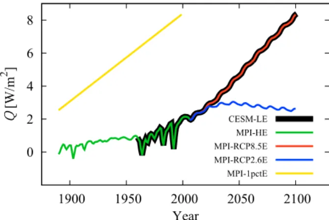
Figure 1gives an overview (Meinshausen et al. 2011) of the forcing scenarios, interpreted in terms of the nominal radiative forcing Q, in the time span of our particular investigations (beginning in 1890; see later).

Note that the nominal radiative forcingQis nota pa- rameter of the system, so that its time dependence is nota forcing from a dynamical point of view. Instead, we treat it as a proxy for the aggregated effect of all different forcing agents (which include different tracers in the atmosphere, as well as the varying solar activity and land use—except for the MPI-1pctE).

To ensure memory loss (i.e., convergence to the snapshot attractor;Drótos et al. 2015;Herein et al. 2016;

Drótos et al. 2017), in most cases we discard the first 40 years of the simulations (the only exceptions are the

FIG. 1. The nominal radiative forcingQas a function of time in the particular simulations within the timespan of our investigation.

For the nominal radiative forcing in the CESM-LE, MPI-HE, MPI- RCP8.5E, and MPI-RCP2.6E, seeMeinshausen et al. (2011). The nominal radiative forcing in the MPI-1pctE has been calculated via the logarithmic response (Ramaswamy et al. 2001).

(4)

simulations forced by the RCP scenarios, which are continuations of the historical simulation). We emphasize that, in principle, a detailed and dedicated investigation should be carried out in both models to determine the time scale of the convergence, as advocated in Drótos et al. (2017). Due to technical limitations, however, this is far beyond the scope of the present study, which we believe to nevertheless provide reliable results with the assumption of maximum 40 years for the convergence time; see Part I of the online supplemental material.

We note that our estimates for the convergence time correspond to the convergence properties that are determined by the atmosphere and the upper ocean with time scales of a few decades, and notthose that characterize the deep ocean and its abyssal circulation, which has time scales of hundreds or thousands of years.

According to this time-scale separation, we conjecture that the adjustment of the slow climate variables corresponding to the abyssal circulation does not influence substantially the statistical properties investigated here.

Note that, otherwise, all the studies on the twenty-first- century climate change performed by looking at the properties of an ensemble of simulations would be hopeless. The details of this time-scale separation in the climate system and its particular implications remain the topic of future research.

3. Characterizing ENSO in a changing climate The phases of ENSO are traditionally characterized by looking at carefully constructed climate indices, which surrogate the dominant features of the behavior of the fields of interest of the climate system. Most directly—and commonly—the sea surface temperature (SST) is considered to characterize the fluctuations of ENSO, which arise in part by oceanic Kelvin waves closely confined to the equator (Dijkstra 2005).

Indices of ENSO, the so-called Niño indices (Trenberth 1997), are defined as the average SST in various rectan- gular regions stretched along the equator, minus the temporal mean of that, then divided by its temporal standard deviation, but traditionally involving some smoothing as well. Thereby, anomalously high and low values of the Niño index are considered as ‘‘episodes’’ or phases of the fluctuation phenomenon, called El Niño and La Niña, respectively (Trenberth 1997). Here we are not concerned with episodes; nevertheless, we will naturally end up with using anomalies in our context (section 4).

What we need to decide about is the equatorial Pacific region of interest. We choose the box 58N–58S, 1508– 908W, which defines the Niño-3 index; that is, we

consider the average SST T_N3 in this box. This is so because we wish to check the consistency of our findings in a given ESM with a previous report on observational data analysis (Krishna Kumar et al. 1999) that considers the Niño-3 index.

To demonstrate the robustness of the detected changes in the ENSO–IM teleconnection in the MPI-ESM, or the lack of that, we also consider the difference, denoted by p_diff, between the seasonal mean of the sea level pressure at Tahiti and at Darwin (p_diff 5 p_Tahiti 2 pDarwin). The differencepdiffis the basis of the Southern Oscillation index (SOI) as defined by the Bureau of Meteorology of the Australian Government, and mea- sures the strength of the Walker circulation. This version, not involving statistical preprocessing of the time series of the sea level pressure before taking their difference, is also called the Troup SOI. An anomalously low (high) value ofp_diff, and so that of the SOI, indicates an El Niño (La Niña) phase (Troup 1965), and, therefore, the SOI (p_diff) is negatively correlated with the Niño-3 (T_N3).

In Part II of the supplemental material, we recall from Herein et al. (2017) that climate indices should be treated carefully in a changing climate. In particular, long-term temporal averaging has to be avoided in their definition, and should be replaced by averaging with respect to the ensemble (after convergence has oc- curred). In the following whenever we mention Niño-3 or SOI, we mean the revised ensemble-wise index/

anomaly when needed: we subtract the ensemble mean from the quantity in question, and divide the result by the ensemble standard deviation. Indices or any anomalies defined in this proper way do not carry information about temporal shifts in the climatic mean of the corresponding original quantities (likeT_N3orp_diff). Therefore, investigations of shifts in climatic means have to be and can be carried out separately from those targeting the internal variability as represented by anomalies only.

We do not investigate the shift of means here, but it can be found inHerein et al. (2018)for a setting somewhat different from here.

4. The ENSO–IM teleconnection in a changing climate of the ESMs: A forced response of internal variability

a. Conceptual considerations

A special aspect of internal variability is the presence of teleconnections: for certain variables characterizing geographically distant regions, anomalies with respect to their climatic mean do not occur independently in a statistical sense. As an example, in the case of ENSO, if

(5)

T_N3(p_diff) is anomalously low (high) during the summer months, there is a good chance that the precipitation of the Indian monsoon is anomalously high, and vice versa (Trenberth 1997). However,Roy et al. (2019) reports that the teleconnection strength can be very different when filtering for canonical, Modoki, or mixed ENSO events. Note that we will primarily consider the June–

August (JJA) average of T_N3and p_diffand the June–

September (JJAS; monsoon season) average of the precipitationPto conform to traditional definitions and because the truly instantaneous quantities would have much lower correlation. We will nevertheless use exactly one data point from each year, which is the time period within which these quantities are defined.

The simplest way to quantify the strength of the (tele-) connection between two given variables is via Pearson’s correlation coefficientr(Rogers and Nicewander 1988).

Note that the correlation coefficient is obtained, by definition, as the average of the product of the anomalies (as defined by subtracting the average and dividing by the standard deviation; cf. the previous section) of the corresponding quantities. Consequently, a correlation coefficient between anomalies is the same as that between the original quantities. Therefore, in our context of the teleconnection, we can speak interchangeably aboutTN3and Niño-3 on the one hand, andpdiffand SOI on the other hand. We underline that Pearson’s correlation coefficient is limited to detect a linear correlation between the two quantities of interest; nonetheless, it is useful for having a first-order picture of the existing correlations in the fields.

InHerein et al. (2017)it has been demonstrated that the traditional evaluation of correlation coefficients, carried out via averaging over time, provides us with grossly incorrect results under a changing climate. It is thus important to evaluate correlation coefficients with respect to the ensemble: in nonautonomous systems with explicit time dependence the two operations are not equivalent. As evaluation over the ensemble can be done atany‘‘instant’’ of time (after convergence), it also enables one to monitor the temporal evolution of the strength of the teleconnection during a climate change.

This temporal evolution is one aspect of the response of internal variability to an external forcing. This is what we shall investigate in this section for the teleconnection between ENSO and the Indian monsoon.

In particular, we numerically evaluate the ensemble- based correlation coefficient between the ‘‘instantaneous’’

JJA averages of the SST (T_N3)—or the sea level pressure difference (p_diff) between (grid points closest to) Tahiti (17831⁰S, 21826⁰E) and Darwin (12828⁰S, 130850⁰E)—and the ‘‘instantaneous’’ JJAS seasonal average precipitation Pover India [except for a few states in order to keep to the

all-India summer monsoon rainfall (AISMR) dataset being our reference; see Fig. 1 ofParthasarathy et al. (1994)];

with the ‘‘option’’ ofp_diffit reads as r5 hp_diffPi2hp_diffihPi

ffiffiffiffiffiffiffiffiffiffiffiffiffiffiffiffiffiffiffiffiffiffiffiffiffiffiffiffiffiffiffiffiffiffiffiffiffiffiffiffiffiffiffiffiffiffiffiffiffiffiffiffiffiffiffiffiffiffiffiffiffi (hp²_diffi2hp_diffi²)(hP²i2hPi²)

q ,

where h. . .i denotes averaging with respect to the ensemble. The time t here, concerning the ENSO–IM teleconnection, is discrete with yearly increments, as explained above; this is why we write ‘‘instantaneous’’

using quotation marks.

Our choice corresponds to investigating the direct (i.e., nonlagged) influence of ENSO on the IM. There also exists an indirect influence (Wu et al. 2012) between the beginning of a given ENSO period (from December to February) and the consecutive Indian summer monsoon. Interestingly, the sign of the correlation coefficient between the ENSO characteristic and the IM precipitation is opposite in this case. Beyond these influences, Wu et al. (2012)also identify a ‘‘coherent’’ influence, with origins in both seasons. These alternatives are, however, out of the scope of the present paper.

b. Numerical results

Since the temporal character of the forcing is quite different in certain ensembles, the results are more easily compared if we plot them as a function of the radiative forcing Q instead of time. One should keep in mind, however, that the response is always expected to exhibit some delay (Herein et al. 2016), and that the nominal radiative forcingQis just a proxy for the aggregated effects of different forcing agents (seesection 2) [this can also be formulated in a rather rigorous way using the formalism of response theory; see discussion inLucarini et al. (2017)].

The results are shown in this representation inFigs. 2a and 2bfor all ensembles considered. Due to the moderate size of the ensembles, especially for the CESM- LE, but also strongly affecting the MPI-ESM ensembles, the numerical fluctuation of the signals is considerable, so much that one cannot read off meaningful coefficients for particular years (corresponding to individual data points in our representation). The structure of the time dependence thus remains hidden. What might be identified, however, from our plots are main trends or their absence, with approximate values on a coarse-grained temporal resolution. Had our ensembles been of infinite size and, thus, able to accurately describe the distribution supported by the snapshot attractor, we would be able to have information at all time scales.

As shown inFig. 2the MPI-ESM ensembles seem to give a rather constant value,jrj’0.5, for the coefficient [both with Niño 3 (T_N3) and SOI (p_diff)], both when

(6)

plotted as a function ofQ(Figs. 2a,b) and when plotted as a function of the time t(Figs. 2c,d). By a visual inspection, no trends can be identified with ‘‘confidence’’

even for the MPI-RCP8.5E or the MPI-1pctE. The magnitude and the sign of the correlation coefficients are in harmony with the observations (Walker and Bliss 1937;Parthasarathy and Pant 1985;Yun and Timmermann 2018). At the same time, the CESM shows very little correlation. Such a large discrepancy is unexpected. For this reason we do not examine the CESM here any further.

Note that the underestimation of the strength of the teleconnection by the CESM agrees withRamu et al. (2018).

After the visual inspection, we take to formally testing if we can reject with high confidence the hypothesis that the correlation coefficient is constant during the timespan of the MPI-ESM simulations, or in any (sub)intervals. Our test is based on the fact that the distribution of the Fisher transform (Fisher 1915,1921) of an estimate of a given correlation coefficientr(i.e., its area-hyperbolic tangent, which we shall denote by z) calculated from a sample (in our case, an ensemble) of given sizeNfollows a known distribution to a very good approximation: a Gaussian with a standard deviation of 1/ ffiffiffiffiffiffiffiffiffiffiffiffi

N23

p , provided that the original quantities also follow Gaussian distributions (Fisher 1936). Should the latter conditions be met, the sampling distribution ofz

would be the same in each year of a given ensemble simulation with the only possible difference appearing in the mean of this distribution. Since calculations described in Part III of the supplemental material support that different years are independent for this single ex- ceptional variable, the setup would become suited for a Mann–Kendall test (Mann 1945;Kendall 1975) for the presence of a monotonic trend in the time series ofz, whereby stationarity would become rejectable. (Note that nonmonotonic time dependence is out of the scope of a single Mann–Kendall test, but testing in different intervals may reveal nonmonotonicity, as discussed below.) To keep simplicity, we evaluate Mann–Kendall tests for z calculated from the original variables in the main text, and give support for the negligible effect of their non- Gaussianity in Part IV of the supplemental material.

We present values of the test statisticZMKto indicate the certainty of the presence of trends and also the sign of detected trends (and show the more commonly usedp values in Part V of the supplemental material). We carry out the test in all possible subintervals of our time series (of annual data points) in order to gain some insight into the possible inner structure of the simulations.

Note that this representation suffers from the so-called multiple hypothesis testing problem enhanced by correlation between neighboring data points of the plot

FIG. 2. The correlation coefficient between the all-India summer monsoon rainfall and (a),(c) Niño-3 or (b),(d) SOI as a function of (top) the nominal radiative forcingQand (bottom) time in different ensembles as indicated by the coloring (seeFig. 1). For comparability,2ris plotted in (a) and (c). For visibility, MPI-RCP2.6E is not included in (c) and (d). Consecutive years are connected by lines in all panels.

(7)

(Wilks 2016); that is, even larger seemingly significant patches may be false detections. However, the point-by- point values of the test statistic are not corrupted, so that the probabilities associated to these values are correct and can be interpreted in the usual way.

Results for Z_MK in the MPI-HE and the MPI- RCP8.5E stitched together can be seen inFigs. 3a and 3b. Such a diagram could indicate if a trend islinearin time, because in that case a stratification of the color chart would be parallel to the diagonal or the hypote- nuse of the right triangle of color. In contrast with this, a

‘‘hockey stick’’–like time dependence would instead result in a horizontal contour of lowpvalues, in association with the start year of the steep change. A further relevant pattern will be a ‘‘dipole’’ ofZ_MKwith an axis parallel to the diagonal, corresponding to the emergence and the subsequent reversal of a trend (a ‘‘bump’’ or a ‘‘ditch’’).

Note that these features aretemporal, as opposed to a possible relationship with the forcing (which might be represented, e.g., by the radiative forcing Q, which is not a linear function of time according toFig. 1).

A steady increase in the teleconnection strength is an attribute more so when Niño-3 characterizes ENSO (as

inFig. 3a) as opposed to the SOI (Fig. 3b). In fact, with the SOI a change is not even detected under the RCP8.5 scenario alone, only if the historical period is included.

A very certain trend begins within the historical period, in the late twentieth century, and can be detected almost irrespectively of the starting point of the interval, like a hockey stick pattern. This is unexpected, as the historical forcing is the weaker one. It is even more interesting to notice a trend with an opposite sign a few decades later: as indicated by the dipole structure, the teleconnection first becomes stronger, and then loses strength.

Note the contrast with the Niño-3-based characterization for which hard significant trends are traced out only in the late twenty-first century: trends in the late twenty- first century are practically absent when using the SOI.

To support the reliability of our methodology, we present analogous results obtained with an independent hypothesis testing technique in Part V of the supplemental material. In a completely different approach, the slopes of linear fits displayed in similar diagrams also trace out the same structure as that ofFigs. 3a and 3b;

seeFigs. 3c and 3d. Even a small-scale organization of the diagrams along vertical and horizontal lines proves

FIG. 3. TheZMKvalues [color coded;jZMKj.1.96 (corresponding topMK,0.05, shown in Fig. S6 in the online supplemental material): red or blue, according to the sign] and slopes calculated in the MPI-HE and MPI-RCP8.5 stitched together for all possible subintervals of the whole time span. ENSO is represented by (a),(c) Niño-3 and (b),(d) SOI.

(8)

to be the same, which suggests that this organization is not an artifact of the methodologies, but is presumably due to the influence of the more outlying values ofz.

The diagrams of the slopes inFigs. 3c and 3dalso give us a first estimate for the strength of assumed monotonic trends. Of course, these are very unreliable along the main diagonal (cf. the low absolute values of Z_MK in Figs. 3a and 3b) but, in statistically significant areas of the plots, they show how sudden the increase and the drop in the teleconnection strength is for the SOI, and that the strengthening is particularly fast in the late twenty-first century for Niño-3.

As a test of robustness, we carry out the same evaluation but exclude September from the monsoon season.

The diagrams of the test statisticZMK(informing about the certainty of the presence of a trend by being nor- mally distributed in the absence of a monotonic trend) and the slopes of linear fits are displayed inFig. 4. We conclude that the general structure of the changes in the correlation coefficient is robust, even if the detectability of change in some specific intervals is not robust.

To link what is seen when using Niño-3 and the SOI, we extend our analysis to two further ENSO characteristics: the Niño-3.4 index, considering the SST farther west in the equatorial Pacific (in the box 58N–58S, 1708–

1208W;Ashok et al. 2007), and the box-SOI, extending the box concept to the atmospheric sea level pressure difference (replacing Tahiti and Darwin by the boxes 58N–58S, 808–1608E and 58N–58S, 1608–808W, respectively;Power and Kociuba 2011). The results for these two choices, shown inFig. 5, are surprisingly similar to each other and, furthermore, exhibit the main features of both of the original choices: a gradual increase in the teleconnection strength with an enhancement in the late twenty-first century (Niño-3) and a ‘‘bump’’ at the turn of the century (SOI). It is thus obvious that both Niño- 3.4 and the box-SOI are some kind of intermediate representation of the ENSO phase between Niño-3 and the SOI from the point of view of the teleconnection with the Indian monsoon.

We further extend our analysis by performing the same evaluation for the MPI-1pctE and for the combination of the MPI-HE and the MPI-RCP2.6E; seeFigs. 6and7, respectively. When using Niño-3, a long-term increase in the teleconnection strength is seen under any forcing. It is re- markable that the strength of the teleconnection keeps increasing even after the peak in the radiative forcing of the RCP2.6 (Fig. 7). When following the RCP2.6 after the historical period, the SOI-based characterization, surprisingly, also ‘‘sees’’ this increasing teleconnection strength

FIG. 4. As inFig. 3, but with September excluded from the monsoon season.

(9)

in the late twenty-first century very well, unlike for the RCP8.5 (Fig. 3). Finally, the MPI-1pctE is completely different from the SOI point of view: the dipole pattern indicates a weakening followed by a strengthening.

5. The ENSO–IM teleconnection in view of observational data

In the context of observations, one is provided with a single historical realization, and therefore no ensemble- wise statistics can be evaluated. The obvious way to check a change in time is to compare statistics belonging to nonoverlapping time windows. A time series can even be obtained by a moving window statistics. There are two approaches to calculating moving cross-correlations.

One is a direct approach, calculating Pearson’s correlation coefficient in any given time window. This way the segment of the time series is ‘‘normalized’’ naturally by the average and standard deviation of this segment.

Because of the removal of the mean, this is sometimes viewed as detrending, besides a filtering out of low- frequency variability. Yun and Timmermann (2018, hereafter YT18) present their result in their Fig. 1b following this approach. Alternatively,Krishna Kumar et al. (1999, hereafterKK99) preprocess the time series,

before applying the direct method, by subtracting a smoothed running mean in a centered window. We note that with the latter approach, the resulting moving correlation time series is shorter by a window size.

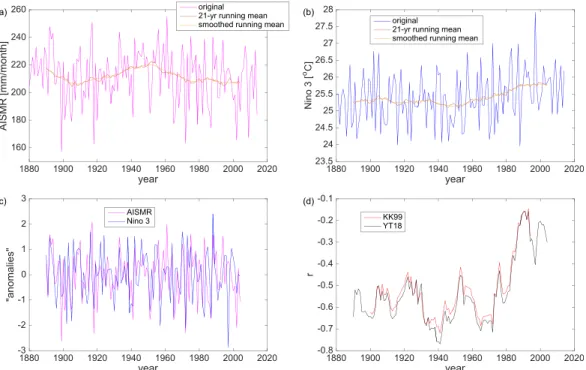
We apply both of these algorithms here, employing a 21-yr window, as didKK99andYT18, although we use a centered window for evaluating the correlation itself, unlike YT18 (and probably also KK99) did without justification. Stages and the result of this are shown in Fig. 8, where we used the ERSST v5 (Huang et al. 2017) and the AISMR (Parthasarathy et al. 1994;Mooley et al.

2016) observational data products for the SST and Indian summer monsoon rainfall, respectively.

Our results do more or less reproduce that ofKK99, except perhaps that we see more variability before 1980.

[On the weakening of the teleconnection in the late twentieth century, see alsoKinter et al. (2002),Sarkar et al. (2004), andBoschat et al. (2012).] It turns out also that the direct method (YT18) results in approximately the same time series in this scenario, except thatris most typically, but not always, larger.

Nevertheless, we examine the robustness of the ‘‘significance’’ of the weakening of the running correlation.

Prompted by the diversity of variables used in the literature, we perturb both the precipitation and SST variable

FIG. 5. As inFig. 3, but for Niño-3.4 and the box-SOI.

(10)

to be correlated with one another, whose results are shown inFigs. 9a and 9b, respectively. By ‘‘perturbation’’

we mean considering alternatives either to the data product or the area over which we calculate the mean.

To start with, instead of the AISMR data, we use the CRU PRE v4.03 (Harris 2019a,b) data (available only over land), masked with the AISMR regions for an exact match in this respect. The different data product does make a difference with respect to the ‘‘significance’’ of weakening, indicating less of it in view of the CRU PRE data. It also matters if instead of a mask given by the shape of India [except for a few states; see Fig. 1 of Parthasarathy et al. (1994)] we take the mean in the box 58–258N, 708–908E (YT18): there is less (more) weakening after 1980 (around 1950). Furthermore, excluding the monsoon rain in September also results in more weakening around 1950. Otherwise, the little difference after 1980 indicates that in this period the monsoon season became shorter.

Using other data products for the SST, on the other hand, namely ERSST v4 (Huang et al. 2015) (as also used by YT18) and HadISST1 (Rayner et al. 2003), makes a difference only before 1940. Finally, considering only the eastern half of the Niño-3 box shows again less weakening after 1980, but leaves the period around 1950 largely unaffected. [We have checked that the

subtraction of a smoothed running mean before calculating the running correlation (KK99) brings about mi- nuscule differences in all cases; results not shown.]

6. Discussion

a. Possible reasons for the apparent discrepancy between model and observations

The contrast between the ensemble-wise (section 4) and temporal (section 5) results obtained for the MPI-ESM and observations, respectively, is constituted by the opposite sign of the change in the strength of the ENSO–IM teleconnection. This disagreement may have different reasons:

1) The ensemble-wise and temporal correlation coefficients do not quantify the same thing.

2) The temporal single-realization result features so much internal variability that it does not actually allow for detecting nonstationarity.

3) The model is not truthful to the real climate.

Regarding point 1 we recall that the ensemble-wise correlation coefficient is an ‘‘instantaneous’’ (yearly) quantity whereas the temporal correlation coefficient is obviously using information from several years. The latter is not really relevant in a changing climate, whereas

FIG. 6. As inFig. 3, but for the MPI-1pctE. Note the shorter length of the simulation.

(11)

the probability of the co-occurrence of the anomalies of the two system components (ENSO and IM) is reflected correctly only in the former, as discussed in the introduction.

As a further aspect of the difference, the ensemble- wiser, unlike the temporal one, does not exclude correlations of low-frequency variability; in principle it could be the case that the latter was strengthening in the twentieth century and it dominated over a weakening correlation of higher-frequency variability.

Regarding point 2 we remark that insection 5we did not pursue hypothesis testing (as we did insection 4) as the time series of moving correlations has an autocorrelation time determined by the window size, and so it does not satisfy, for example, the assumption of the Mann–Kendall test. While this may be circumvented by restricting the investigation to nonoverlapping windows, such a technique makes obvious that the autocorrelation introduced by windowing seriously reduces the effective sample size. For instance, even if the original time series ofrlacks autocorrelation, a 21-yr windowing of a 140-yr time series results in an effective sample size of no more than 7, approximately. Nevertheless, it is surprisingly common to see in publications an incorrect report on the

significance of, say, trends despite these aspects. It appears to us thatKK99also disregarded these considerations when they claimed that the weakening of the teleconnection is significant in a statistical sense. Indeed, if the detection of trends or nonstationarity in this context is already challenging when endowed with a 63- member ensemble (section 4), it seems hopeless from a single realization. See also Wunsch (1999),Gershunov et al. (2001), andYun and Timmermann (2018).

Nevertheless, it would be very valuable to be able to rely on temporal statistics, by which observational climate data could be analyzed. As climate models can represent some aspects of the climate inaccurately, our only chance to gain an understanding of those aspects is by analyzing observational data. Ben Santer advocates (2019, personal communication) that the great value of ensembles of climate model simulations, like the MPI- GE or CESM-LE, is that they can serve as a testbed for temporal statistics or algorithms. For example, one can check how well ergodicity is satisfied in some given context, which is known (Drótos et al. 2016) to be not satisfied in a generic nonautonomous case.

Returning to point 1 in this respect, we can simply evaluate the temporal correlations for all 63 converged

FIG. 7. As inFig. 3, but for the MPI-RCP2.6E stitched after the MPI-HE. Note that the lower triangles are identical to those inFig. 3.

(12)

members of the MPI-GE, and see if they typically feature aweakeningteleconnection likeKK99reported.

Figure 10 shows the result with both kinds of ‘‘detrending.’’ We see that the ensemble average temporal correlation [a quantity also evaluated by Mamalakis et al. (2019)] is rather steadilyincreasingin the historical period, which lets us conclude that the disparate treat- ment of low-frequency correlations does not bring about

a typical opposite trend here. Nevertheless, the different behavior of the ensemble-mean temporal correlation under RCP8.5—increasing with the indirect method of KK99 and stagnating with the direct method of YT18—cautions us to keep an open mind about unexpected differences.

The same figure also addresses the possibility of point 2. The variances of the moving correlations are very

FIG. 8. Moving temporal correlation coefficient based on observational data (see also the main text): (a) JJAS all- India summer monsoon rainfall data; (b) JJA mean Niño-3 index based on the ERSST v5 dataset. In both of these diagrams a 21-yr running mean is shown as well as a smoothing of it obtained by the Savitzky–Golay filter (of order 3 and a window size of 21 years, applying Matlab’s ‘‘sgolayfilt’’). This is what is subtracted from the original data, in ways of detrending, followingKK99. (c) ‘‘Anomalies’’ obtained followingKK99, providing visuals of correlation.

(d) The correlation coefficient itself, obtained by both the direct method ofYT18and the method ofKK99.

FIG. 9. Moving temporal correlation coefficient, followingYT18, based on various observational variable combinations. Robustness is examined by ‘‘perturbing’’ both the (a) precipitation and (b) SST variables. The legends indicate the following combinations: #1: ERSST v5, AISMR; #2: ERSST v5, CRU PRE masked with the AISMR regions; #3: ERSST v5, CRU PRE in the box 58–258N, 708–908E (YT18); #4: (ERSST v5, AISMR JJA only;

#5: HadISST1, AISMR; #6: ERSST v4, AISMR; and #7: ERSST v5 eastern half of Niño-3 box, AISMR.

(13)

large, but it is also not very unlikely to have a smaller variance for many decades followed by a drift (i.e., a considerable apparent weakening or strengthening of the teleconnection). We find examples for this among the 63 ensemble members. Actually, it is recognized in many studies (Kinter et al. 2002; Ashrit et al. 2003;

Sarkar et al. 2004;Ashrit et al. 2005;Annamalai et al.

2007; Kitoh 2007;Chowdary et al. 2012; Li and Ting 2015) that ‘‘modulations’’ and corresponding apparent trends in the studied correlation coefficient, when calculated over different time intervals [as done by, e.g., Boschat et al. (2012)andR. Li et al. (2015)] or over moving (sliding) time windows [as done by, e.g.,Krishna Kumar et al. (1999),Ashrit et al. (2001),Kinter et al.

(2002),Ashrit et al. (2003),Ashrit et al. (2005),Annamalai et al. (2007),Kitoh (2007),Chowdary et al. (2012), and Li and Ting (2015)], can appear as a result of internal variability. In particular,Li and Ting (2015)conclude that the observed weakening of the teleconnection in the late twentieth century would be due to internal variability.Sarkar et al. (2004)go beyond this saying, on the basis of physical arguments, that ‘‘the effect of ENSO on Indian precipitation has not decreased but on the con- trary it has increased in recent times’’ (p. 4), aligning, in fact, to our finding in the MPI-GE, but claiming that actual strengthening was dominated by internal variability seeing a weakening.

Finally, we address the possibility of model errors, point 3. We start with presenting maps of global SST trends for the historical period inFig. 11, comparing the MPI-ESM and observations. All-year data are used to fit a straight line whose slope represents the trend. As for the model, we show both the ensemble average and standard deviation of the trends.

Like some earlier versions (Collins et al. 2005), the version of the MPI-ESM used to generate the MPI-GE seems to have a La Niña–like warming, that is, more

warming in the western than in the eastern equatorial Pacific. Considering the ensemble-wise variance globally, the observed warming (and cooling) trends seem to be consistent with the model. Note that the observed equatorial Pacific warming, like the ensemble mean in the MPI-GE, is La Niña–like, and it is in disagreement with the report ofLian et al. (2018)on a cooling instead, even if in the eastern equatorial Pacific. We do not pursue here rigorously (Wilks 2016) the question of the (in)consistency of these patterns, although it should be clear that it would be just a matter of dataset size to detect inconsistency.

We continue with similar maps of JJAS precipitation climatology over India shown inFig. 12. It is clear that the model has less rain over land, possibly partly because of its coarser resolution, so that high mountains that

‘‘force’’ precipitation are not resolved. Increasing model resolution has been plausibly indicated byAnand et al.

(2018)to reduce model biases (see their Fig. 6) also over the sea. The latter might be a clue that, due to the con- servation of water, negative precipitation bias over high mountains and positive biases nearby over the ocean can be related. Considering the ensemble-wise variability too, the discrepancy can be indeed considered a bias, not just a difference by chance or statistical error.

However, the patterns between model and observations certainly bear a resemblance. The patterns for the trends, on the other hand, are less similar; seeFig. 13.

Furthermore, the magnitude of some local trends in the observation exceeds by far anything in any realization of the model.

While this might be a clue to the origin of the discrepancy between a possible weakening temporal correlation in observations and a typically strengthening one in the model, we emphasize that a temporal correlation of detrended data is hoped to quantify some relationship between fluctuations rather than forced trends

FIG. 10. Moving temporal correlation coefficient for all converged members of the MPI-GE in the historical period continued seamlessly with the RCP8.5 forcing scenario, following both (a)KK99and (b)YT18. The thin gray lines show all the realizations while three realizations are shown in color, providing examples. Thick blue lines show the ensemble average of the temporal correlation, which are blown up in insets to better indicate any trend.

(14)

of the climatic mean signal. Nevertheless, in conclusion, if the discrepancy is to do with model errors (point 3), then it is more likely coming from the side of the precipitation than the SST.

However, when regarding the particular quantities at the basis of our analyses of the teleconnection, Fig. 14a shows that the average Indian monsoon rainfall in the model and observations seem to have

FIG. 12. Climatological JJAS mean precipitation in model and observation. (a) Ensemble mean and (b) standard deviation of the JJAS mean precipitation in the MPI-HE (1880–2005). (c) JJAS mean precipitation in the CRU PRE (1900–2010) dataset (data available only over land).

FIG. 11. Climatological SST trend in model and observation. (a) Ensemble mean and (b) standard deviation of the SST trend in the MPI-HE (1880–2005). (c) SST trend in the ERSST v5 (1880–2016) dataset.

(15)

consistent fluctuation characteristics and perhaps also trend, even though the underestimation of the rainfall by the model is also seen from this angle. The Niño 3 index orTN3, shown inFig. 14b, can be described very similarly: despite a 28C cooler model, the variance and temporal characteristics of the fluctuations seem to closely resemble each other in the model and observations.

b. The nonlinearity of the response and possible reasons for that

In view of the Niño-3–AISMR correlation (see, e.g., Figs. 3a,4a, and6a) the possibility that the forced response of the teleconnection would be approximately linear cannot be excluded. However, representing ENSO by the sea surface temperature just in a somewhat more westerly box

FIG. 13. As inFig. 12, but for long-term temporal trends of JJAS mean precipitation.

FIG. 14. Comparison of large-area averages in model (MPI-ESM) and observation (precipitation: AISMR, magenta; SST: ERSST v5, blue): (a) JJAS precipitation and (b) JJA SST. To match the AISMR data, precipitation in the model is averaged over the AISMR areas (India, except for a few states; see main text). The JJA SST is averaged over the Niño-3 box. Thin gray lines represent all converged members of the MPI-GE, while three colored lines show examples of individual members; the thick blue lines show the ensemble mean.

(16)

(Niño-3.4), or, by the SOI, nonlinearity—and what is more, nonmonotonicity—becomes obvious (see, by contrast,Figs. 3b,4b,5b, and6b). We shall first discuss possible reasons for nonlinearity even if the forcing might be considered relatively weak in all scenarios (from the point of view of response theory;Ruelle 2009;

Lucarini et al. 2017). Remember that temporal line- arity has to be distinguished from a linear response to forcing, but nonmonotonicity in Fig. 5 excludes both options. We also recall that the teleconnection keeps strengthening even after radiative forcing peaks in RCP2.6 (seeFig. 7).

In the slightly different setup ofHerein et al. (2018), considering precipitation only in the northernpart of India, from an analysis of the sensitivity of hypothesis tests to stationarity, we concluded that the strength of the teleconnection in view of the SOI cannot respond to the radiative forcing Q instantaneously and linearly, since otherwise those tests would have had to detect nonstationarity also in the MPI-RCP8.5E alone and the MPI-1pctE (beyond the MPI-HE), which was not the case.

Some very strong form of nonlinearity could explain the results in principle. However, another possible ex- planation lies in the radiative forcingQnot being a dynamical forcing (i.e., a single quantity that appears explicitly in the equations of motion). That is, a causal response function might not exist between Q(as pre- dictor) andr(as predictand;Lucarini 2018).

In particular, the strength of the teleconnection may respond in a different way to variations in different forcing agents. Remember that the nominal radiative forcing Q represents the aggregated effects from several different agents, and responses might not be possible to be interpreted in terms of variations in the single quantityQ. The underlying mechanisms might even turn out to be not or not directly related to the increase in the net energy flux.

In fact, the differentiation of responses with respect to different forcing agents would not be very surprising. As shown byBódai et al. (2018)by considering a (globally homogeneous) CO2 forcing alone, while the resulting Qmight act as a dynamical forcing with respect to the surface temperature, it does not do so, for example, with respect to the temperature at the tropopause (Bódai et al. 2018). The teleconnection of ENSO with the Indian summer monsoon might indeed involve a physical mechanism not restricted to the surface, or to observables that would secure the causality of the ‘‘response’’ of the teleconnection toQ. If we add that the response in the climatic mean of the Indian summer monsoon has actually been found byLi and Ting (2015; however, by utilizing techniques based on temporal averaging) to be

governed by different mechanisms under aerosol forcing (related to volcanism, or, indeed, large-scale pollution in South and Southeast Asia) and greenhouse gas forcing, we can easily imagine that the fluctuations of the Indian summer monsoon respond differently to these two kinds of forcings, causing the teleconnection to respond in a different way, too.

Note that volcanism is enhanced in the late twentieth century when changes in the strength of the teleconnection are first prominently seen in the MPI-GE. In fact, a hypothesis has been put forward byMaraun and Kurths (2005)that after major volcano eruptions in the southwest Pacific the ‘‘cooling effect could reduce the land/sea temperature gradient and thus make the Monsoon more sensitive to ENSO influence’’ (p. 4). These authors found more regular oscillatory ENSO dynamics and a phase locking between ENSO and the monsoon in the observed time series after major volcano eruptions in southern Indonesia, which, they claim, should be reflected in an increased correlation, perhaps (see below) consistent with our finding. This could also be an indication that a single realization contains already a lot of information about the forced response in terms of a nonlinear quantifier of the teleconnection, as opposed to Pearson’s

‘‘linear’’ correlation coefficient. Taking into account that the pure ensemble-based description of teleconnections is the statistically most relevant one and is usually more robust than single-realization temporal techniques, it might prove to be extremely fruitful to carry out an ensemble-based analysis but replacing Pearson’s correlation coefficient by e.g., Spearman’s ‘‘nonlinear’’ rank correlation coefficient.

Nevertheless,Maraun and Kurths (2005)claim to not disagree withKK99about the decrease of the correlation strength as a forced response. They describe a transition near 1980 from a 1:1 phase locking into a 2:1 phase locking, with the Indian monsoon oscillating twice as fast. This connection, they claim, would be ‘‘invisible to (linear) correlation analysis,’’ or rather the correlation would be destructed by the additional monsoon peak. Note, however, that nonstationarity is not yet verified for observations (section 6a), so that the picture might be more complicated than sketched byMaraun and Kurths (2005). From this point of view, it could be checked if the MPI-ESM features the same effect in terms of the phase difference analyzed by them.

The above discussion shows many possibilities for a nonlinear response. However, we have also found considerable variations in the results when choosing different characteristics of ENSO. Nevertheless, a long- term increase in the ENSO–IM teleconnection strength is present ineveryscenario when utilizing an area-based index. Furthermore, a ‘‘bump’’ is also rather consistently

(17)

detected under the combination of the historical and RCP8.5 forcings at the turn of the century if the ENSO characteristic is based on some more western part of the Pacific. It is only for the pressure differencep_diffbetween two grid points that a rather erratic behavior is found.

Such a quantity should be more sensitive when the spatial patterns playing the main role in the teleconnection phenomenon are not simple and when these patterns change substantially even if the bulk does not.

While the analysis of changes in the ENSO pattern [usually investigated by empirical orthogonal functions (EOFs)] may already prove to be informative, the patterns most relevant for the teleconnection can be identified by the ‘‘maximal covariance analysis’’ (MCA) or

‘‘canonical correlation analysis’’ (CCA). One can evaluate these also ensemble-wise, similarly to the recently developed snapshot EOF technique (SEOF; Haszpra et al. 2020), by which changes in these patterns can be studied or detected. [See the SEOF’s application to ENSO inHaszpra et al. (2020); one may call the new techniques SMCA and SCCA.] In principle, it may still be that such analyses yield a different picture depending on using the SST or the sea level pressure to characterize ENSO. We will investigate these matters as future work.

Acknowledgments. The authors wish to express grati- tude to J. Broecker, C. Franzke, T. Haszpra, T. Kuna, N.

Maher, S. Milinski, and T. Tél for useful remarks and dis- cussions. GD is thankful to B. Stevens, T. Mauritsen, Y.

Takano, and N. Maher for providing access to the output of the MPI-ESM ensembles. The authors also wish to thank the Climate Data Gateway at NCAR for providing access to the output of the CESM-LE. The constructive feedback from three reviewers is greatly acknowledged, most im- portantly their suggestion of considering an SST-based index, beside the sea-level-pressure-based SOI, to represent ENSO. TB wishes to thank Kyung-Sook Yun for sharing with him some of the preprocessed observational data used inYun and Timmermann (2018)and pointing him to other data sources. Funding: The simulations for the MPI- RCP8.5E were supported by the H2020 grant for the CRESCENDO project (Grant 641816). MH is thankful for the great support of the DFG Cluster of Excellence CliSAP. This research was supported by the National Research, Development and Innovation Office, NKFIH, under Grants PD124272, K125171, and FK124256. GD was supported by the Ministerio de Economía, Industria y Competitividad of the Spanish Government under Grant LAOP CTM2015-66407-P (AEI/FEDER, EU), and by the European Social Fund under CAIB grant PD/020/2018

‘‘Margalida Comas’’. TB, VL, and FL were supported by the H2020 grants for the CRESCENDO (Grant 641816) and Blue-Action (Grant 727852) projects. VL has been

supported by the DFG Sfb/Transregio TRR181 project.

TB was also supported by the Institute for Basic Science (IBS), under IBS-R028-D1.

REFERENCES

Anand, A. S. K. Mishra, S. Sahany, M. Bhowmick, J. S. Rawat, and S. K. Dash, 2018: Indian summer monsoon simulations:

Usefulness of increasing horizontal resolution, manual tuning, and semi-automatic tuning in reducing present-day model biases. Sci. Rep., 8, 3522, https://doi.org/10.1038/s41598-018- 21865-1.

Annamalai, H., K. Hamilton, and K. R. Sperber, 2007: The South Asian summer monsoon and its relationship with ENSO in the IPCC AR4 simulations.J. Climate,20, 1071–1092,https://doi.org/

10.1175/JCLI4035.1.

Arnold, L., 1998:Random Dynamical Systems. Springer-Verlag, 586 pp.

Ashok, K., S. K. Behera, S. A. Rao, H. Weng, and T. Yamagata, 2007:

El Niño Modoki and its possible teleconnection.J. Geophys.

Res.,112, C11007,https://doi.org/10.1029/2006JC003798.

Ashrit, R. G., K. Rupa Kumar, and K. Krishna Kumar, 2001:

ENSO–monsoon relationships in a greenhouse warming scenario.Geophys. Res. Lett.,28, 1727–1730,https://doi.org/10.

1029/2000GL012489.

——, H. Douville, and K. Rupa Kumar, 2003: Response of the Indian monsoon and ENSO–monsoon teleconnection to enhanced greenhouse effect in the CNRM coupled model.J. Meteor. Soc.

Japan,81, 779–803,https://doi.org/10.2151/jmsj.81.779.

——, A. Kitoh, and S. Yukimoto, 2005: Transient response of ENSO–monsoon teleconnection in MRI-CGCM2.2 climate change simulations.J. Meteor. Soc. Japan,83, 273–291,https://

doi.org/10.2151/jmsj.83.273.

Bellenger, H., E. Guilyardi, J. Leloup, M. Lengaigne, and J. Vialard, 2014: ENSO representation in climate models: From CMIP3 to CMIP5.Climate Dyn.,42, 1999–2018,https://doi.org/10.1007/

s00382-013-1783-z.

Bittner, M., H. Schmidt, C. Timmreck, and F. Sienz, 2016: Using a large ensemble of simulations to assess the Northern Hemisphere stratospheric dynamical response to tropical volcanic eruptions and its uncertainty.Geophys. Res. Lett.,43, 9324–9332,https://

doi.org/10.1002/2016GL070587.

Bjerknes, J., 1969: Atmospheric teleconnections from the equatorial Pacific.Mon. Wea. Rev.,97, 163–172,https://doi.org/10.1175/

1520-0493(1969)097,0163:ATFTEP.2.3.CO;2.

Bódai, T., and T. Tél, 2012: Annual variability in a conceptual climate model: Snapshot attractors, hysteresis in extreme events, and climate sensitivity.Chaos,22, 023110,https://doi.org/10.1063/

1.3697984.

——, G. Károlyi, and T. Tél, 2011: Fractal snapshot components in chaos induced by strong noise. Phys. Rev. E, 83, 046201, https://doi.org/10.1103/PhysRevE.83.046201.

——, V. Lucarini, and F. Lunkeit, 2018: Critical assessment of geoengineering strategies using response theory.Earth Syst.

Dyn. Discuss.,https://doi.org/10.5194/esd-2018-30.

Boschat, G., P. Terray, and S. Masson, 2012: Robustness of SST teleconnections and precursory patterns associated with the Indian summer monsoon.Climate Dyn.,38, 2143–2165,https://

doi.org/10.1007/s00382-011-1100-7.

Branstator, G., and H. Teng, 2010: Two limits of initial-value de- cadal predictability in a CGCM.J. Climate,23, 6292–6311, https://doi.org/10.1175/2010JCLI3678.1.