Pannon Egyetemen
EFOP-3.4.3-16-2016-00009
H-8200 Veszprém, Egyetem u.10.
H-8201 Veszprém, Pf. 158.
Tutorial for Operations Research:
Modeling in GNU MathProg
András Éles, György Dósa
Faculty of Information Technology University of Pannonia, Veszprém, Hungary
2019
Contents
1 Introduction 3
2 Optimization 6
2.1 Equations . . . 6
2.2 Finding the „Best” solution . . . 7
2.3 Main concepts . . . 8
2.4 Mathematical programming . . . 10
3 GNU MathProg 12 3.1 Prerequisites for programming . . . 12
3.2 „Hello World!” program . . . 13
4 Equation systems 19 4.1 Example system . . . 19
4.2 Modifications in code . . . 21
4.3 Parameters . . . 23
4.4 Data blocks . . . 24
4.5 Indexing . . . 28
4.6 Other options for data . . . 33
4.7 General columns . . . 36
4.8 Minimizing error . . . 38
4.9 Equation systems – Summary . . . 42
5 Production problem 43 5.1 Basic production problem . . . 43
5.2 Introducing limits . . . 50
5.3 Maximizing minimum production . . . 55
5.4 Raw material costs and profit . . . 58
5.5 Diet problem . . . 61
5.6 Arbitrary recipes . . . 64
5.7 Order fulfillment . . . 75
5.8 Production problem – Summary . . . 89
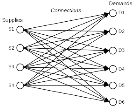
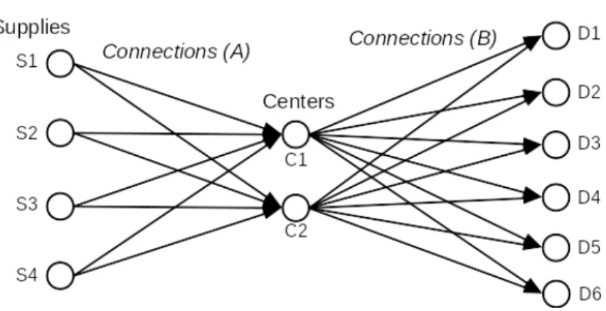
6 Transportation problem 90 6.1 Basic transportation problem . . . 90
6.2 Connections as index set . . . 95
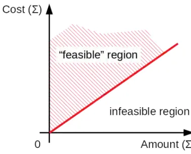
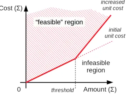
6.3 Increasing unit costs . . . 98
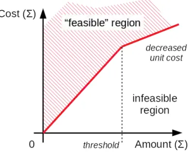
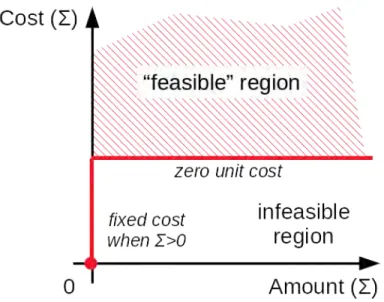
6.4 Economy of scale . . . 102
6.5 Fixed costs . . . 108
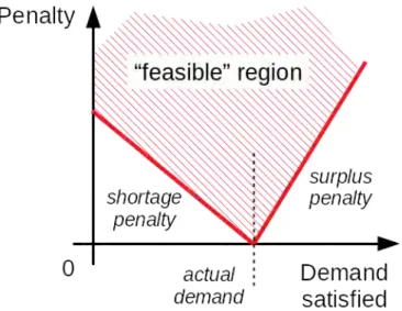
6.6 Flexible demands . . . 111
7 MILP models 123
7.1 Knapsack problem . . . 123
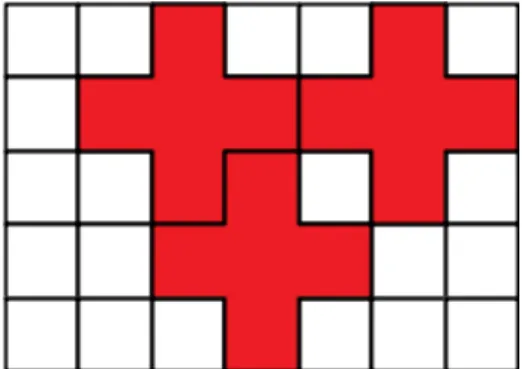
7.2 Tiling the grid . . . 130
7.3 Assignment problem . . . 139
7.4 Graphs and optimization . . . 145
7.5 Travelling salesman problem . . . 155
7.6 MILP models – Summary . . . 165
8 Solution algorithms 166 8.1 The Primal Simplex Method . . . 166
8.2 The Two-phase (Primal) Simplex Method . . . 170
8.3 The Dual Simplex Method . . . 171
8.4 The Gomory Cut . . . 172
9 Summary 175
Chapter 1
Introduction
This Tutorial is intended to give an insight into mathematical programming, and Operations Re- search in general, through the development of Linear Programming (LP) and Mixed-Integer Linear Programming (MILP) models using the GNU MathProg (GMPL) modeling language.
Optimizationmeans finding the most suitable solution in real life situations. This is often pos- sible using common sense or some simple logic, but there are many cases where advanced approaches are needed. Usually a mathematical model of the problem is considered, and solution methods are designed utilizing the best of the available mathematical theoretical background, computer theory and existing technology.
The problem is generally the vast number of possible solutions to a problem, which are impossible to be all taken into account one by one, even with the fastest computers available. In many situations, instead of a perfect solution, „rules of thumb”, also called heuristic methods are used. These simplify the underlying model of the problem, trim the set of possible solutions to be investigated or both.
This sacrifices optimality but makes finding a fairly good solution of the problem computationally possible. Nevertheless, even in these cases, finding such a solution usually requires some optimization to be made, for example to find the best solution from a few candidates.
If an optimization problem is faced, a „conventional” method of solving is the design, implemen- tation and application of a specificalgorithm, which usually require some programming language.
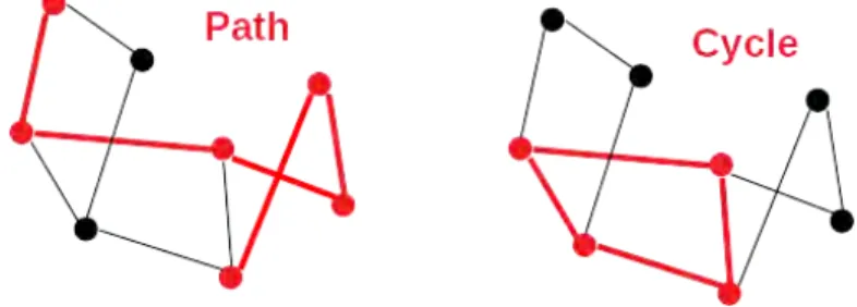
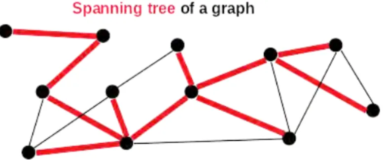
The concept of algorithm has a very general meaning, and it also depends on what programming language we choose to implement it, but usually the data structures used and the steps to be made are described. This is what most common programming languages can do, for example C/C++, Java, Python, etc. The common point in these languages is that not only the „What?” is answered by implementing the algorithm, but the „How?” is also addressed by the programmer. That is, the exact steps to be made with the data are described. For example, Dijkstra’s algorithm can find the shortest path in a graph, Kruskal’s algorithm can find the cheapest spanning tree of a graph, or the Ford-Fulkerson algorithm is capable of finding the optimal flow in a flow network.
Mathematical programming methods are an alternative. Instead of describing the steps to be made, only the mathematical model of the real-world problem is formulated. The mathematical model consists of statements like equations, inequalities, logical expressions and more, which corre- spond to the rules governing the real-world problem and its solution. Then, the real-world problem is solved by finding solutions to the system of these equations, inequalities or other statements.
However, only the formulation of the mathematical model is up to the programmer, not the algo- rithm of how it is solved. The latter is actually done by somesolversoftware, which is designed to solve a particular class of mathematical programming models.
In this Tutorial, a subset of mathematical programming methods, namely Linear Program- ming (LP)andMixed-Integer Linear Programming (MILP)models are in scope, which can be formulated by the GNU MathProg (GMPL) modeling language [1]. Tackling real-world opti-
mization problems by formulating a mathematical programming model and solving it with a solver software is a valuable expertise that is substantially different from programming in the „conven- tional” way. Nevertheless, an algorithm designed to solve a specific optimization problem may be much faster than a mathematical programming model: many well-studied optimization problems have state-of-the-art algorithmic solutions. However, for some problems, even for some where decent algorithms exist, designing a mathematical programming model instead can be surprisingly fast and easy. Mathematical programming models are also more flexible in case the real-world problem itself is changed.
The algorithms that the solvers utilize to actually solve our formulated mathematical program- ming model are on their own an interesting subject, but is not in focus. In short, the way these models can be formulated are more important than how these mathematical models can be solved to optimality.
The modeling language GNU MathProg is selected because, along with its solver glpsolin the GNU Linear Programming Kit [2], these are tools relatively easy to be understood, and available under the GNU General Public License. There are many other free, and commercial tools for both formulating and solving not only MILP, but more general mathematical programming models. Many of such tools are much faster thanglpsol.
There are several other learning materials available in this subject. The basic installation of GLPK also includes a bunch of example models, including complex ones. GLPK also has a Wik- ibooks project where usage is covered in high detail [3]. We would like to recommend the Linear Programming tutorial of Hegyháti [4]. Moreover, many useful books and lecture materials can be found at the Hungarian Tankönyvtár homepage [5].
This Tutorial presents the basics of the language, and some key problems that can be easily solved by mathematical programming tools, to give an insight into the strength of optimization with mathematical, and particularly MILP models. Some algorithmic solution methods for particular problems are also presented.
The rest of the Tutorial is organized as follows.
• Chapter 2 provides the introduction to the main goals, tools and concepts of optimization.
• Chapter 3 introduces to the basic usage of GNU MathProg and solver glpsol. A minimal,
„Hello, World!” model file is shown.
• In Chapter 4, linear equation systems are solved using GNU MathProg with gradually improv- ing model implementations. This part aims at demonstrating features of the language that are required to develop concise and general LP/MILP models, most importantly indexing and the separation of model and data sections.
• Chapter 5 introduces the production problem, a simple optimization problem. Incremental development of models is in focus, demonstrated through changes, extensions of the problem definition. Some additional language features, and integer variables are used.
• Chapter 6 shows another simple optimization problem, the transportation problem. Modeling techniques for some cost functions are presented, which can be part of more complex problems.
• Chapter 7 mentions some harder problems requiring MILP model formulations. Advanced modeling and coding techniques, and possible graphical outputs are presented.
• Chapter 8 gives an insight into the LP/MILP solving algorithms, explaining briefly how soft- ware tools may work in the background.
This Tutorial contains attachments. All GNU MathProg codes including model and data files, and its outputs mentioned in the text can be found, grouped by chapters and sections. (A more detailed description is available in the attachment itself.)
INTRODUCTION
For learning purposes, it is recommended to manually see, and solve the models with their corresponding data file(s) to investigate the results. Note that most of the codes and more important output file segments are included in the text of the Tutorial itself, full or in part, using a specific format.
GNU MathProg code of model files is formatted like this.
GNU MathProg code of data sections that may go to separate data files are formatted like this.
Output generated by the solver is formatted like this.
Commands to be run are formatted like this.
If you have questions, or in case you find any errors in this Tutorial, please feel free to contact us ateles@dcs.uni-pannon.hu. We hope you will find this material useful.
Optimization
2.1 Equations
Equationsare one of the easiest and strongest mathematical modeling tools we have. Let’s see an example problem that can be solved by an equation.
Problem 1.
Alice’s train departures 75 minutes from now. She lives 3 km away from the station and wants to walk, but she and also needs 30 minutes to get ready. How fast shall she walk to the station to catch the train?
We can see that what we actually seek is the minimal average speed Alice have to move with.
She can be faster at some points of her walk, or slower, but overall, the average speed counts, determining when she will arrive. She can even go with constant speed to achieve the same result.
Also, we seek to find the minimal speed, with which she just catches the train. Of course, she can be even faster, then she will have some waiting time at the station. These steps may be trivial, but are also part of the modeling procedure: we simplified the problem into finding a single minimal speed value and we may assume that Alice goes with that constant speed, and just catches the train.
The problem can be solved by expressing the time until she arrives to the station intwo different ways. Once, the time she arrives is75 min, by the train schedule. On the other hand, the time she arrives is30 minfor getting ready, plus the time she walks. The latter term is something which is not known, it depends on Alice’s speed. Now, we introduce a variablexto express Alice’s speed, which is in question. Variablexis some value that can be chosen, that Alice has freedom upon. She can choose her speed in order to arrive to the station sooner or later.
With x, we can express the time she spends walking easily by 3 kmx . Now an equation can be formulated based on the fact that Alice’s arriving time is expressed in two different ways.
30 min +3 km
x = 75 min (1)
The task for Alice is to choose an appropriatexso that this equationholds. From this point, the equation is formulated, we can forget the real-world problem and apply our mathematical knowledge about solving equations. This is an easy one. We can, for example, subtract 45 minutes from both sides, multiply byx (which, we can assume not to be zero), then dividing by3 km, in that order.
We arrive to the following.
4km
h =x (2)
2.2. FINDING THE „BEST” SOLUTION OPTIMIZATION
What we actually do by solving an equation is transforming it to easier forms so that the next form is a direct consequence of the previous. The final form isx= 4kmh , which literally means the following: „If 30 min + 3 kmx = 75 min, then its direct consequence is x= 4kmh ”. So, if Alice just catches the train, then her average speed is 4kmh And at this point we finally got the result and interpreted it in the reality. This is the general way on how equations are used in problem solving.
First, we identify the freedom we have at the problem to be solved (x, the speed). Then, we use equations, as modeling tools to express the rules of reality that must be obeyed (the first equation).
The model is now ready, we apply our solution techniques which can be quite general for any kinds of equations and have nothing to do with the underlying real-world problems. In this case, the equation is transformed in a chain of direct consequences until the variable is expressed directly as a constant value. Finally, if the result is obtained for the mathematical model, we interpret it as the solution of our initial real-world problem.
Of course, there are much more difficult examples of equation solving (for example, multiple solutions for single equations, fake solutions, multiple variables, multiple equations at the same time, etc.), which are not covered here. But the point is that the scheme is similar each time: we formulate a mathematical model that describes the real-world situation, solve that model with some well-known general techniques and then interpret the solution of the model as the solution of the original problem.
2.2 Finding the „Best” solution
Note that the question about Alice catching the train in Problem 1 was how fast she can go to catch the train. The answer wasx= 4kmh , but that is not totally correct. Actually,x= 5kmh ,x= 10kmh or evenx= 15kmh are solutions as well for her, if she can run that fast. However x= 3kmh is not a solution, as she will miss the train if she is that slow. Of course, for this particular problem, we understand that there is a minimum speed of x= 4kmh , for which Alice just catches the train in time. However, the more precise formulation would be the following inequalityinstead.
30 min +3 km
x ≤75 min (3)
Two quantities are here: the time Alice needs to reach the station if her speed is x, that is, 30 min +3 kmx , and the time the train departs, 75 min. These two quantities are related: Alice must arrive before or exactly when the train is due (not later, in other words). This can be expressed as an inequality rather than an equation, but the goal is the same. We must find a speed for Alice x for which the inequality holds. Technically, this can be done exactly the same way as the equation itself was solved, leading tox≥4kmh . That means that the solutions are actually allxspeeds that are at least 4kmh . There are infinitely many solutions for the inequality, so infinitely many speeds Alice can choose.
Now this is more precise, but Alice may be interested in the minimum speed she can choose, so letxbe as small as possible. The formulation is as follows.
minimize : x
subject to : 30 min +3 kmx ≤75 min (4) At this point, the formulated problem is anoptimizationproblem. The goal is not only finding one suitable solution for a real-world problem, but finding the most suitable one in some aspect.
In the mathematical point of view, optimization is not only finding a solution for an equation, inequality, or a set of such, but finding the best. Optimization is a sub-field of Operations Research, as it is an inevitable way of supporting business decisions: given a complex real-world situation, what shall be the best response?
2.3 Main concepts
Now that we have seen some optimization from Problem 1, it is time to establish some basic concepts of optimization models.
When solving a real-world problem by defining some variables, equations, inequalities, etc. we formulatea mathematicalmodelfor the problem. That model is then solved with mathematical knowledge, that is usually independent of the original, real-world problem. If the solution procedure is made by some software (usually the case), that software is called a solver.
There are variablesin an optimization model. These represent our freedom of choice: the way the variable can take different values represent our different actions. In Problem 1, there is a single variable,xrepresenting Alice’s average speed.
A solution of an optimization model is when all the variables take some value. If there are multiple variables in the model, then a single solution consists of values for all of these variables.
Two solutions are considered different if any of the variables take a different value. In Problem 1, there are infinitely many solutions, like x= 4kmh , x= 10kmh , and moreover, x= 1kmh as well (see below), although Alice misses the train.
Usually the variables cannot take arbitrary values. In Problem 1, Alice cannot choose a speed if she would miss the train with it. Such restrictions that must apply, are called constraints. So in the example problem, there is a single constraint, which is expressed by Inequality 3.
There are a wide range of constraints that may appear in an optimization problem, some cannot even be expressed as inequalities. The concept of boundsshall be mentioned: these are constraints that require a single variable to be not less than, or not more than a given constant limit. For example, x ≥ 0kmh is a bound that must also be ensured. The problem required Alice to move with a positive speed, so it was implicitly enforced and neglected. In many optimization problems, however, we must explicitly consider bounds, otherwise solutions might not reflect reality. Bounds also have a great practical importance in model solution algorithms.
Constraints decide whether solutions are feasibleorinfeasible. A feasible solution is when all variables take a value for which all the constraints hold. Otherwise, it is an infeasible solution. In Problem 1, solutions x= 4kmh and x= 10 kmh are feasible, whilex= 1kmh is infeasible. We could also say that, literally,x= 4kmh is a solution andx= 1kmh is not a solution, but we rather use the terminology of feasible and infeasible solutions.
The way we distinguish feasible solutions of a model so that whether they are more or less suit- able, is expressed in the model as anobjectivefunction, which is to be minimized (or maximized).
An objective function - like constraints - evaluates an expression based on the model variables. The goal of optimization is to find a feasible solution for which the objective function is minimal (or maximal). A solution with this property is an optimal solution of the model. If a solution is optimal, then we can be sure that any other solutions are either infeasible, have an equal or worse objective value, or both. There can be multiple optimal solutions for the same model. In Problem 1, we have a very simple objective functionc(x) =x, which is minimal at the solution ofx= 4kmh . The optimal objective for the problem is therefore4kmh . Sometimes we refer to the objective value as the solution of an optimization problem. Therefore, we can say that the optimal solution of Problem 1 is 4kmh .
It may happen that an optimization model does not have a feasible solution at all, hence there are no optimal solutions either. In this case, we say the model is infeasible. For example, the following modification of the problem (see Problem 2), the resulting System 5 would be infeasible:
Alice is too far away and cannot go fast enough, she will miss the train by 3 minat least.
Problem 2.
Alice’s train departures 75 minutes from now. She lives 8 km away from the station and wants to walk, and also needs 30 minutes to get ready. Also, she cannot run faster than10kmh in average.
How fast shall she walk to the station to catch the train?
2.3. MAIN CONCEPTS OPTIMIZATION
minimize : x
subject to : 30 min +8 kmx ≤75 min x≤10kmh
(5) In rare cases, it may appear that a model is unbounded. This means that there are feasible solutions but none of them are optimal, because there are even better and better feasible solutions as well. For example, if the goal for Alice was to go as fast as possible to catch a train, instead of being as slow as possible, then neither4kmh ,10kmh ,1000kmh or the speed of light would be optimal solutions, because there would always be a feasible solution with higher speed value. Of course, this does not make sense. Usually, when our model turns out to be unbounded, then we either made a mistake in solving it, or it does not describe reality well – maybe because it misses some real-world constraint we did not thought about. The latter was the case in our example, because in practice, Alice cannot go as fast as she wishes.
We can also call the set of feasible solutions of the model as thesearch space, emphasizing that our actual goal in optimization is to maximize or minimize an objective function value over the set of feasible solutions. Also, if all the variables together are treated as a mathematical vector, then each solution can be considered a point in that vector space. The set of all feasible solutions is a set of points in space that might have some special properties. For example, in LP problems, it is a convex polytope. Constraints (and bounds) are used to define the search space. Each constraints might exclude some feasible values from the search space that are no longer feasible anymore because of that constraint.
It may appear that there is a constraint that does not exclude solutions from the search space at all. We call those constraints redundant. Note that redundant constraints do not affect the solutions of the model, and hence the optimal solution, but may affect the solution procedure itself, either in a positive or a negative way. We may also refer to constraints as redundant if they do actually exclude some solutions, but only those which are not interesting for us (for example, because they cannot be optimal for some reason and therefore will not be reported by the solution algorithm anyways).
Now see a bit more elaborate example for an optimization problem.
Problem 3.
A company wants to design a new kind of chocolate in the form of a rectangular brick of ho- mogeneous material. They want the brick to contain as much mass as possible, however, there are regulations on the faces of the brick, for transporting considerations. One of the faces must have an area not greater than6 cm2, another face cannot be greater than8 cm2, and the largest face cannot be greater than12 cm2. What is the largest mass for a piece of chocolate?
This example can be part of a business decision problem. The company wants to maximize its profit, but has to find a suitable solution for production. Operations Research helps in decision making, for example, with optimization models.
Now it is not even straightforward to define the variables themselves. Though not even mentioned in the problem text, the three edges of the brick, say x, y and z are adequate, for the following reasons. From these we can easily express the other quantities the problem specification refers to:
xy,xz andyzare the faces, and xyzis for the total volume which is to be maximized. Note that if the chocolate is homogeneous, then volume is proportional to mass, so we may consider maximizing volume instead of mass, they are equivalent. Second, x,y andzare independent of each other: the selection of x does not directly affect the selection of y, as all possible combinations can yield a brick. If they were not independent, additional constraints must have been formalized.
The most important thing is that if x, y and z are given, then the solution to the real-world problem is well-defined. That means, we can exactly tell whether the constraints are satisfied or not, and what the objective value is. This is the most important requirement for a set of variables
to be adequate for a model. Now let us do this work: express the three constraints for the faces and the objective of the volume to formulate the optimization model. Note thatx,y andz should also be positive, but these bounds will be implicitly enforced by an optimal solution of the model.
maximize : xyz subject to : xy≤6 cm2
xz≤8 cm2 yz≤12 cm2 x, y, z≥0
(6)
There are many feasible solutions for this model, for examplex=y=z= 2 cmis a feasible one, but x=y=z = 2.5 cmis an infeasible one. There is a single optimal solution, which is x= 2 cm, y= 3 cmandz= 4 cm, the total volume in this case is24 cm3.
The way of finding this optimal solution and undoubtedly prove that it is indeed optimal, is not trivial, and is out of scope of this Tutorial. There is a hint, if the reader liked to solve it:
(xyz)2=xy·xz·yz.
2.4 Mathematical programming
We have seen two very simple optimization problems so far, however, for the latter one we would have been in trouble if we had to actually solve it and prove that our solution is indeed optimal.
However, the point of mathematical programmingis that we are not the ones who actually solve the models. We are the ones who translate the real-world problem to an optimization model, then usually a software designed generally for solving models is doing the dirty job for us. Finally, we only need to verify that the solution of the model is actually a suitable solution to the real-world problem.
A mathematical programming model consists of the model variables that represent our freedom of choosing solutions, the constraints that express the requirements for a solution to be feasible, and correspondingly, suitable in the real-world problem, and finally the objective function, which determines the criteria of finding the best among the feasible solutions.
Although the general idea is that we are only formulating a model, we still need to take care about what class of model we choose. The main reason is that it greatly affects what kind of solution methods we can use. Solving a model from a more special class in contrast with a more general one can be drastically cheaper in terms of computational effort. We explicitly mention two model classes that are of great importance in Operations Research.
InLinear Programming (LP) models, the variables can take arbitrary real values. The con- straints are equations or non-strict inequalities of linear expressions of the variables. A linear expression is the sum of some of the variables, each multiplied by a constant. Linear expressions cannot contain multiplication, division of the variables with each other, or any other mathematical functions or operations: only addition, subtraction, and multiplication by a constant is allowed.
The objective function itself must be a linear expression of the variables, the minimization or max- imization of which is the optimization goal. The following is an example of an LP problem.
minimize : 3x+ 4y−z subject to : 2x+ 5 =z+ 2
x−y≤0
x+y+z≤2 (x+y) x, y, z≥0
(7)
One important thing about LP models is that only non-strict constraints are allowed (≤, ≥or
=), but strict constraints (<,>) are not. Also note that Problem 1 about Alice is formulated as an
2.4. MATHEMATICAL PROGRAMMING OPTIMIZATION
LP model, while Problem 3 about the chocolate bricks is not LP, because it contains a product of variables, which is a nonlinear term.
An LP model is solvable in polynomial time in the number of constraints and variables. That means, large models can be formulated and solved in acceptable time with a modern computer. LP problems have several interesting properties that make them solvable with efficient algorithms, for example, the Simplex Method (see Chapter 8). One of such properties is that the set of feasible solutions in space is always a closed, convex set.
InMixed-Integer Linear Programmingmodels, we may additionally restrict some variables to only take integer values in feasible solutions, contrary to LP problems. This difference makes solving generally the wider class of MILP models an NP-complete problem in the number of integer variables. That means, if there are many integer variables in an MILP model, then we generally cannot expect a complete solution in acceptable computational time. However, the number of applications the class of MILP models can cover is surprisingly more extended than for LP problems, making MILP models a popular method for solving complex optimization problems. There are effective software tools utilizing heuristic algorithms that usually solve not too complex MILP models very fast.
In this manual, we focus on MILP and LP models. In both cases, there are only linear expressions of the variables appearing in the formulations. There are other problem classes like Nonlinear Programming (NLP), Mixed-Integer Nonlinear Programming (MINLP), with corresponding solvers, but these are not covered here.
GNU MathProg
This chapter aims at briefly introducing GNU MathProg and how it can be used to implement and solve mathematical programming models in the LP or MILP class. A short example problem is presented with implementation, solution and results, with some of the most frequently used features of the language shown.
3.1 Prerequisites for programming
GNU MathProg, also referred to as the GNU Mathematical Programming Language, or GMPL, is a programming language for designing and solving LP and MILP. The GNU Linear Programming Kit, GLPK provides free software to both parsing implemented models and solving them until the optimal solution is reported. GLPK is available under the General Public License version 3.0 or later [6].
There are other software tools for solving MILP models, some are available with a free license like CBC, or lpsolve. These mentioned can be much faster than GLPK. Commercial software can even be better, some of them are available through academic license. However, we selected GNU MathProg and solver glpsol from GLPK because it is relatively easy to use and includes both language and model solving tools.
Installing GLPK depends on the operating system. On Linux, we can head to the official website of GLPK, where installation packages, source codes and even sample GNU MathProg problems can be found. On some distributions, installation can be done with a single command as follows.
sudo apt-get install glpk-utils
If installation is complete, we shall have the program glpsol available in the command line.
Throughout this manual, we will use this tool to parse and solve models, in command line.
On Windows, there is a possibility to obtain the command line solver as well. However, a more convenient option is a desktop application called GUSEK [9], which is a simple IDE with text editor for the GNU MathProg programming language. The solver glpsol is available with all of its functionalities there. With GUSEK, no command line is needed, although navigating between multiple files requires some attention.
Reference manual for the GNU MathProg modeling language with usages of theglpsolsoftware is publicly available, see the references [1].
3.2. „HELLO WORLD!” PROGRAM GNU MATHPROG
3.2 „Hello World!” program
After successful installation, we can try the program with a very simple LP problem. This will be our first GNU MathProg program, like a „Hello World!”.
var x >= 0;
var y >= 0;
var z >= 0;
s.t. Con1: x + y <= 3;
s.t. Con2: x + z <= 5;
s.t. Con3: y + z <= 7;
maximize Sum: x + y + z;
solve;
printf "Optimal (max) sum is: %g.\n", Sum;
printf "x = %g\n", x;
printf "y = %g\n", y;
printf "z = %g\n", z;
end;
GNU MathProg is designed to be easy to read, and the mathematical meaning to be easy to understood. The language consists of commands ending with a semicolon (;), these are called statements. There are six distinct statements in this file: var, s.t., maximize, solve, printf andend. The meanings of most are self-explanatory, as we will see.
var x >= 0;
var y >= 0;
var z >= 0;
First of all, this is an LP problem, all three variablesx, y and z can take real values. Also, they haveboundsdefined: each of them must be nonnegative. Note that this is the most common bound for variables.
s.t. Con1: x + y <= 3;
s.t. Con2: x + z <= 5;
s.t. Con3: y + z <= 7;
In the problem, there are three constraints, apart from the bounds, which are treated differently in the language. The constraints are namedCon1,Con2,Con3, respectively. The names are preceded by „s.t.”, but it has several aliases, it can be „subject to”, or can be omitted at all. The constraints state that the sum of any two of the three variables cannot be greater than given constants, which are3, 5and7, respectively.
maximize Sum: x + y + z;
The goal of the optimization is to maximize the objective entitled as „Sum”, which is, of course, the sum of the three variables. There can be at most one maximize or minimize statement in a model file.
At this point, the LP problem is well defined. This is a relatively easy linear problem, however, its optimal solution might be not obvious for first sight.
It shall be noted that the objective function can be omitted at all from a GNU MathProg model formulation. In this case, the only task is to find any feasible solution for the problem.
solve;
printf "Optimal (max) sum is: %g.\n", Sum;
printf "x = %g\n", x;
printf "y = %g\n", y;
printf "z = %g\n", z;
end;
There is asolve statement in the file. This denotes the point where the solver software should finish reading all the data, then constructing and solving the model. After the solve statement, there may still be other statements in the file, to report valuable information about our solution.
In this case, the objective value and our three variables are printed with their values obtained by the optimization procedure. Theprintf statement works similarly to theprintf()function from the C programming language, but has less supported format specifiers. We prefer the %gformat, because it can print both integers and fractional values in a short form. In some cases, a fixed precision number is more adequate, like%.3f.
An endstatement denotes the end of the model description, although it is optional.
We can use any text editor we like, but some of them have syntax highlight options. GUSEK on Windows has its own text editor which is specifically designed to modeling. On Linux, we can use gedit. It does not have a syntax highlight for GNU MathProg by default, but one can be obtained from the internet.
Let us name this exact file as helloworld.mod. On some systems, the file extension .mod can be recognized as a video format by the file browser. This causes the „double-click” opening method to try to open the file as a video instead of a text file. For this reason, it is recommended to set the opening method of the file to the text editor we prefer, for example gedit. Alternatively, we can simply use a different file extension, like.m, or simply.txt, it does not matter from the viewpoint of glpsol, although it may matter if we use some IDE for programming like GUSEK.
File helloworld.mod is a model file, because it contains the business logic of the problem we want to solve. It is alone enough for defining a problem. Later on, we will split our problem formulations to a single model file and one or moredata files. The model file encapsulates the logic of the problem, while the data file(s) provide the actual data the problem shall be solved with. This will be useful, because if the data of the real-world problem changes, we do not need to tamper with the model itself. In other words, a user who wants to solve a model for a particular problem does not need to know the model, only a data file must be implemented correctly, which is much easier and less error-prone.
Useglpsolto solve the model file with the following command.
glpsol -m helloworld.mod
Something similar to the following output is obtained.
GLPSOL: GLPK LP/MIP Solver, v4.65
Parameter(s) specified in the command line:
-m helloworld.mod
3.2. „HELLO WORLD!” PROGRAM GNU MATHPROG
Reading model section from helloworld.mod...
20 lines were read Generating Con1...
Generating Con2...
Generating Con3...
Generating Sum...
Model has been successfully generated GLPK Simplex Optimizer, v4.65
4 rows, 3 columns, 9 non-zeros Preprocessing...
3 rows, 3 columns, 6 non-zeros Scaling...
A: min|aij| = 1.000e+00 max|aij| = 1.000e+00 ratio = 1.000e+00 Problem data seem to be well scaled
Constructing initial basis...
Size of triangular part is 3
* 0: obj = -0.000000000e+00 inf = 0.000e+00 (3)
* 3: obj = 7.500000000e+00 inf = 0.000e+00 (0) OPTIMAL LP SOLUTION FOUND
Time used: 0.0 secs
Memory used: 0.1 Mb (102283 bytes) Optimal (max) sum is: 7.5.
x = 0.5 y = 2.5 z = 4.5
Model has been successfully processed
This is a small problem, therefore the result is almost instantaneous. Let us observe what information can be read from the output.
GLPSOL: GLPK LP/MIP Solver, v4.65
Parameter(s) specified in the command line:
-m helloworld.mod
Reading model section from helloworld.mod...
18 lines were read Generating Con1...
Generating Con2...
Generating Con3...
Generating Sum...
Model has been successfully generated
The first section of the output is printed during the model generation procedure. Note that if the model has bad syntax, it is remarked here. Only the first error is displayed. It can also be observed that the constraints and objective are the model elements that must be „generated”.
GLPK Simplex Optimizer, v4.65 4 rows, 3 columns, 9 non-zeros Preprocessing...
3 rows, 3 columns, 6 non-zeros Scaling...
A: min|aij| = 1.000e+00 max|aij| = 1.000e+00 ratio = 1.000e+00 Problem data seem to be well scaled
Constructing initial basis...
Size of triangular part is 3
* 0: obj = -0.000000000e+00 inf = 0.000e+00 (3)
* 3: obj = 7.500000000e+00 inf = 0.000e+00 (0) OPTIMAL LP SOLUTION FOUND
Time used: 0.0 secs
Memory used: 0.1 Mb (102283 bytes)
The solution procedure of an LP problem from the constraints themselves to the final, optimal solution is itself an interesting subject of Operations Research. However, we do not focus on the underlying solution algorithms themselves. However, basic knowledge about it would help us de- bugging in the future. First of all, all LP problems are represented in a matrix of coefficients, the rows of which are corresponding to constraints (and the objective), the columns corresponding to variables, and the entries of the matrix being the coefficients of a given variable in a given constraint.
On this matrix, some preprocessing steps are performed, and then the main algorithm is launched.
There are two rows in this output which show a „current” result. The first one shows an objective of 0, the second shows the objective 7.5 which is actually the final optimal solution. The row
„OPTIMAL LP SOLUTION FOUND” denotes that the solver succeeded in solving the problem, and is now aware of the optimal solution and the corresponding values of the variables. If there are multiple optimal solutions, one of them is chosen.
With more complex problems, solution can take a considerable amount of time and current best solutions are regularly displayed. The solution procedure may be ended before arriving to the optimal solution, in which case the best feasible solution found so far is reported. This happens, for example, when a time limit is set to glpsoland it is exceeded during the procedure.
Optimal (max) sum is: 7.5.
x = 0.5 y = 2.5 z = 4.5
Model has been successfully processed
Finally, we can see the result of the printf statements that we added at the end. We can see that the optimal solution is x= 12 = 0.5, y = 52 = 2.5, z = 92 = 4.5, and then the objective function is x+y+z = 152 = 7.5. This result means we cannot choose values for the variables to obtain a larger sum, unless at least one of the constraints (or bounds) are violated. Note that printfstatements are also valid before thesolvestatement, that is, during the model construction procedure. However, before the solve statement, variables and the objective are not available, as they had not been calculated by that point. The final Model has been successfully processed message hints us that the solver call was successful.
We shall also note thatglpsolcommand line tool has many other options available. For example, we can ourselves print an automated solution file with the -ooption. We can also save the output of the program with the--logoption. Also, the constructed model can be exported to formats that other MILP solvers can use. For example, with the--wlpoption, we can export toCPLEX-LPmatrix format, which is supported by many other solver software. Perhaps we do want to use glpsol to solve the model, we only need it to translate the model to some other format. Then, the --check option ensures that the model is only parsed, but not solved. It is also possible to manipulate the solution procedure in many ways.
Now that we have successfully formulated, solved and analyzed the output for our first LP problem implemented in GNU MathProg, let us make a slight change in the model file. Add the
3.2. „HELLO WORLD!” PROGRAM GNU MATHPROG
integer restriction to all three of the variables, as follows. The modified file is now saved as helloworld-int.mod.
var x >= 0, integer;
var y >= 0, integer;
var z >= 0, integer;
From now, this is no more an LP model, but an MILP model, because some (in particular, all) of the variables must take integer values. Solving the model with glpsolis the same.
glpsol -m helloworld-int.mod
The solver identifies the model as MILP, and there are some changes in the generated output.
Solving LP relaxation...
GLPK Simplex Optimizer, v4.65 3 rows, 3 columns, 6 non-zeros
* 0: obj = -0.000000000e+00 inf = 0.000e+00 (3)
* 4: obj = 7.500000000e+00 inf = 0.000e+00 (0) OPTIMAL LP SOLUTION FOUND
Integer optimization begins...
Long-step dual simplex will be used
+ 4: mip = not found yet <= +inf (1; 0)
+ 6: >>>>> 7.000000000e+00 <= 7.000000000e+00 0.0% (2; 0) + 6: mip = 7.000000000e+00 <= tree is empty 0.0% (0; 3) INTEGER OPTIMAL SOLUTION FOUND
Time used: 0.0 secs
Memory used: 0.1 Mb (124952 bytes) Optimal (max) sum is: 7.
x = 1 y = 2 z = 4
Model has been successfully processed
We can observe that a so-called LP relaxation is solved first, the output for which seems the be the same as the output for our initial LP problem. Actually, this is the nature of the solution algorithm, it is first solved as if all the integer restrictions were removed, as an LP problem. Then, the actual MILP model is solved, and we find that the optimal solution is only 7.0 instead of the optimal solution of the LP, which was7.5.
This is not surprising. The only difference between the two models is that the integer problem is more restrictive about the variables. That means, any solution to the MILP is a solution to the LP. But the opposite is not true, as the optimal solution of the LP, x= 0.5,y = 2.5, z= 4.5 was eliminated by the integer restrictions. The LP relaxation is an important concept in solving MILP models - for example, it can be used as a good initial solution, trying to make all the variables to obtain integer variables. Also, if the integer variables all turn out to have integer values in the LP relaxation, then it is guaranteed to be an optimal solution for the MILP as well, because the MILP is the more restricted.
In this model, the solver needed a little extra work for the MILP, and found the solution of x= 1, y = 2and z= 4. Note that it is an optimal solution, but not the only one. x= 0, y = 3, z= 4, andx= 0,y= 2,z= 5are also feasible and optimal solutions with the same objective value of7.0.
As we could suspect, the algorithmic procedure behind the MILP can be substantially more complex than that of an LP. However, the difference in the formulation is only the integer restrictions of the variables.
We should keep in mind that solvers can handle a large number of variables and constraints of an LP model, but usually they can only handle a limited number of integer variables of an MILP model. The exact limit for integer variables strongly depends on the model itself, it can range from dozens to thousands.
Chapter 4
Equation systems
In this chapter, basic capabilities of the GNU MathProg language are presented on an example modeling problem, which is the general solution of linear equation systems. The aim is to navigate from the initial point of a straightforward implementation to the usage of indexing and separated model and data sections.
With this knowledge, maintenance of code, and solution of the model with different instances (different data) become very easy, provided that first the model is correctly implemented. This is the standard way we intend to implement models in the future.
Note that solving linear systems of equations is considered a routine task. There are plenty of capable software tools, either standalone or embedded. A well-known algorithm is the Gaus- sian elimination [10]. But we are now interested in not the solution algorithms, but modeling.
Particularly, GNU MathProg implementation techniques, in this chapter.
4.1 Example system
Let us start with the solution of a small system of equations, now in GNU MathProg.
Problem 4.
Solve the following system of equations in the real domain.
2 (x−y) =−5 y−z=w−5
1 =y+z x+ 2w= 7y−x
(8)
Although it is not explicitly mentioned in the problem description, there are four variables, x, y,z,w, and the real domain means that all of these can take arbitrary real values, independently.
Our goal is to find values for these four variables so that all four equations are true.
If a complete analysis about the problem was in question, then the problem would be not only to find a single solution, but to find all of them - and if there are infinitely many solutions, then characterize this infinite set, moreover, also prove that there are no other solutions. However, for the sake of simplicity, now we only want to find any single solution to the system of equations and we do not want to decide whether there is another or not.
This is therefore a feasibility problem, it means that only a single feasible solution is to be found. There is no need to objective function for which we want to optimize, because there are no
better or worse solutions.
It can be observed that Problem 4 describes alinear system of equations. This is apparent after we arrange the equations into the following format.
2x −2y =−5
y −z −w =−5
y +z = 1
2x −7y +2w = 0
(9)
The point is that this arrangement can be obtained from the original system by simplifying each equation alone: removing the parentheses, adding and merging terms at both sides. In this way, the arranged system is equivalent to the original. On the left-hand side (LHS)of the equation, there is a linear expression of the variables (each multiplied by a constant, then added), and on the right-hand side (RHS), there is a constant, in each equation. Therefore all equations are linear.
If we further add zero terms and emphasize coefficients at each column of the arranged format, we get the following, equivalent form of the same system.
(+2)·x + (−2)·y + 0·z + 0·w =−5 0·x + (+1)·y + (−1)·z + (−1)·w =−5 0·x + (+1)·y + (+1)·z + 0·w = 1 (+2)·x + (−7)·y + 0·z + (+2)·w = 0
(10)
Although this representation is less readable, it represents more generally what a system of linear equations actually mean. For each equation, there is a constant right-hand side, and a linear expression at the left-hand side, for which we only want to know the coefficients for each variable.
So this whole problem can be represented in a matrix of coefficients, for which the rows correspond to solutions, and columns correspond to variables – except the rightmost column, which corresponds to the right-hand side.
This is very close to what we call the standard form of a Linear Programming problem.
The standard form also includes ≥ 0 bounds for all variables, consists of ≤ inequalities instead of equations, and of course, has a linear objective function. This matrix-like form is important because it inspires solution algorithms. However, we are now not going into the details of solution algorithms, neither in case of system of equations nor in LP problems.
Instead, the representation shown in Equation system 10 will be useful to understand the general scheme behind systems of linear equations, and to implement a separated GNU MathProg MILP model, for which a data section describing an arbitrary system of linear equations can be provided and solved.
Now let us see how the code looks like in GNU MathProg. First, the most straightforward implementation is shown, without arrangement of the equations.
var x;
var y;
var z;
var w;
s.t. Eq1: 2 * (x - y) = -5;
s.t. Eq2: y - z = w - 5;
s.t. Eq3: 1 = y + z;
s.t. Eq4: x + 2 * w = 7 * y - x;
solve;
4.2. MODIFICATIONS IN CODE EQUATION SYSTEMS
printf "x = %g\n", x;
printf "y = %g\n", y;
printf "z = %g\n", z;
printf "w = %g\n", w;
end;
As we can see here, GNU MathProg allows usage of parentheses and basic operations, provided that the constraints, now named Eq1, Eq2, Eq3 and Eq4, simplify into an equality (or non-strict inequality) between two linear expressions.
If we solve the above model file, then the solutionx= 0.5,y= 3,z=−2andw= 10is obtained.
This solution is unique, so all solution methods shall end up with this exact result. We can also manually check that all four equations are satisfied with the resulting values of the variables. The code itself helps us by printing the values of the four variables to the solver output.
Now, if the aligned version is to be implemented, we can get the following.
s.t. Eq1: 2 * x + (-2) * y + 0 * z + 0 * w = -5;
s.t. Eq2: 0 * x + 1 * y + (-1) * z + (-1) * w = -5;
s.t. Eq3: 0 * x + 1 * y + 1 * z + 0 * w = 1;
s.t. Eq4: 2 * x + (-7) * y + 0 * z + 2 * w = 0;
As we can see, white space characters can be freely used in GNU MathProg to help with readabil- ity. Also, zero coefficient terms can be eliminated from the expressions and padded with whitespace instead. The rest of the model file can remain unchanged. The result when solving this arranged model file shall be the same.
4.2 Modifications in code
Now that we have a working model file solving a particular system of linear equations, let us try to solve another one, which is obtained by slight modifications from the original one. The problem description is the following.
Problem 5.
Take the equations defined by Equation system 4 as initial, within its aligned form described in either Equation system 9 or 10. Then, obtain another system by applying the following modifications.
1. Change the coefficient ofxeverywhere from 2 to4. 2. Addz in Eq1 with a coefficient of3.
3. Deletey fromEq2 (zeroize its coefficient).
4. Change the RHS ofEq3 to1.5. 5. Add a fifth variablev, with no bounds.
6. Add the equationx+ 3v+ 0.5 =−2z asEq5. 7. Introducev inEq4 with a coefficient of 5.
8. Print out the newly introduced variablev after thesolve statement as the others.
These modifications can be done one-by-one in a straightforward way until the following model is obtained.
var x;
var y;
var z;
var w;
var v;
s.t. Eq1: 4 * x + (-2) * y + 3 * z + 0 * w + 0 * v = -5;
s.t. Eq2: 0 * x + 0 * y + (-1) * z + (-1) * w + 0 * v = -5;
s.t. Eq3: 0 * x + 1 * y + 1 * z + 0 * w + 0 * v = 1.5;
s.t. Eq4: 4 * x + (-7) * y + 0 * z + 2 * w + 5 * v = 0;
s.t. Eq5: 1 * x + 0 * y + 2 * z + 0 * w + 3 * v = -0.5;
solve;
printf "x = %g\n", x;
printf "y = %g\n", y;
printf "z = %g\n", z;
printf "w = %g\n", w;
printf "v = %g\n", v;
end;
The solution of the new system is x= 2,y= 3.5,z=−2, w= 7,v= 0.5. Although not proven here, but this solution is unique.
Now observe which kind of modifications we have to implement in code to obtain the results.
The first four tasks were just replacing, introducing and erasing coefficients from the corresponding equations. In these cases, one must find the corresponding constraints, the corresponding variable in it and apply the changes.
However, the introduction of the new variable requires some more work besides declaring vas a variable with no bounds. If we wanted to maintain the arrangement of the equations, then all must be expanded with a single column for coefficients of v. These coefficients are initially zero, for not being used. Then, in Eq4 and Eq5, we can insert a nonzero coefficient for v afterwards. We also need to manually modify the printing code after thesolvestatement to involvev.
Insertion of the new equation Eq5 would also require some more work. Again, if we wanted to keep the code easy to read and maintain the arrangement, the new code line for Eq5 must be formatted accordingly.
Although this was still a small problem, we can feel that modification of a system of equations to accommodate another problem might be a bit frustrating. It gets worse if the number of variables and equations increase – note that several thousands of both are still considered a problem with reasonable size.
One problem is that the model code includes some redundancy – we have to maintain arrange- ment to preserve readability, although it is not possible for very large problems. However, the greatest drawback is that we have to understand and tamper with model code – although we only need to change the actual problem itself, which is still a system of linear equations.
It would be wise to somehow separate the modeling logic of systems of linear equations, and actual data of the linear equations to be solved (that is, the number of variables, equations, coefficients and right-hand side constants). This is exactly what we will do in the next sections. Afterwards, what we only need is to alter the data, and the model can remain unchanged, which helps us in reusing code in the future, and implementation of problems with large data.
4.3. PARAMETERS EQUATION SYSTEMS
4.3 Parameters
The first thing we do to separate problem data from the model logic is the introduction of param- eters. This case, the modified problem is to be implemented. We only change the code, not the underlying problem.
Parameters can be introduced with the param statement. It is similar in syntax to the var statement for introducing variables. However, theparamstatement defines constant values that can be used in the model formulation. Parameters are by default numeric values, and are used here as such, but note that they can also represent symbolic values (like strings).
The fundamental difference is that variables are the values to be found by the optimization procedure, to satisfy all constraints and optimize a given objective function. For the implementation point of view, the values of variables are only available after the solvestatement. Parameters, on the other hand, are constant values that are initially given, and are typically used to formulate the model itself.
Note that parameters defined by the param statement, similarly to variables defined in thevar statement, must have a unique name, and they can only be used in the model file after definition.
Hence, in any expression, we can only refer to parameters which are defined earlier in the code. For this reason, parameter definitions typically precede constraint and even variable definitions.
First, we only introduce parameters for the right-hand values of the equations, as follows.
var x;
var y;
var z;
var w;
var v;
param Rhs1 := -5;
param Rhs2 := -5;
param Rhs3 := 1.5;
param Rhs4 := 0;
param Rhs5 := -0.5;
s.t. Eq1: 4 * x + (-2) * y + 3 * z + 0 * w + 0 * v = Rhs1;
s.t. Eq2: 0 * x + 0 * y + (-1) * z + (-1) * w + 0 * v = Rhs2;
s.t. Eq3: 0 * x + 1 * y + 1 * z + 0 * w + 0 * v = Rhs3;
s.t. Eq4: 4 * x + (-7) * y + 0 * z + 2 * w + 5 * v = Rhs4;
s.t. Eq5: 1 * x + 0 * y + 2 * z + 0 * w + 3 * v = Rhs5;
solve;
printf "x = %g\n", x;
printf "y = %g\n", y;
printf "z = %g\n", z;
printf "w = %g\n", w;
printf "v = %g\n", v;
end;
From now on, if we need to modify the RHS of an equation, we do not need to modify the code of the constraint describing that equation. Instead, we only need to replace the definition of the given RHS parameter.
In the same manner, we can also introduce parameters for the coefficients of the equations. Be- cause there are coefficients for all5equations and all5variables, a total of25additional parameters are needed.
var x;
var y;
var z;
var w;
var v;
param Rhs1 := -5;
param Rhs2 := -5;
param Rhs3 := 1.5;
param Rhs4 := 0;
param Rhs5 := -0.5;
param c1x:=4; param c1y:=-2; param c1z:= 3; param c1w:= 0; param c1v:= 0;
param c2x:=0; param c2y:= 0; param c2z:=-1; param c2w:=-1; param c2v:= 0;
param c3x:=0; param c3y:= 1; param c3z:= 1; param c3w:= 0; param c3v:= 0;
param c4x:=4; param c4y:=-7; param c4z:= 0; param c4w:= 2; param c4v:= 5;
param c5x:=1; param c5y:= 0; param c5z:= 2; param c5w:= 0; param c5v:= 3;
s.t. Eq1: c1x * x + c1y * y + c1z * z + c1w * w + c1v * v = Rhs1;
s.t. Eq2: c2x * x + c2y * y + c2z * z + c2w * w + c2v * v = Rhs2;
s.t. Eq3: c3x * x + c3y * y + c3z * z + c3w * w + c3v * v = Rhs3;
s.t. Eq4: c4x * x + c4y * y + c4z * z + c4w * w + c4v * v = Rhs4;
s.t. Eq5: c5x * x + c5y * y + c5z * z + c5w * w + c5v * v = Rhs5;
solve;
printf "x = %g\n", x;
printf "y = %g\n", y;
printf "z = %g\n", z;
printf "w = %g\n", w;
printf "v = %g\n", v;
end;
Note that param statements can be put in a single line for the sake of readability, and to preserve the arrangement of the equations. After the total of 30 parameters are introduced, the implementation of the equations can be considered final. With the sole modification of the parameter statements in the model file, we can solve arbitrary systems of linear equations with5variables and 5 equations.
Note that the solution of any of these two models are exactly the same as before, as the system of equations itself did not change, only its implementation.
4.4 Data blocks
We had separated the coefficients and RHS values from the equations they are in, but still, we need to modify theparam statements in the model file to alter the problem. We used a single model file
4.4. DATA BLOCKS EQUATION SYSTEMS
each time so far. Now we introduce the concept of themodel sectionand thedata section, with which we can separate the model logic with the problem data entirely.
Parameter values in GNU MathProg can be determined in two ways.
• A parameter value is explicitly given where it is defined: as a constant value, or some expression of other constant values, other parameters, and built-in functions and operators of the GNU MathProg language.
• A parameter value in not given in the model section, but in a separate data section.
Now let us see how we can modify the model file to obtain a separate model section and data section. In case where only the RHS parameters were introduced, the complete separation is the following.
var x;
var y;
var z;
var w;
var v;
param Rhs1;
param Rhs2;
param Rhs3;
param Rhs4;
param Rhs5;
s.t. Eq1: 4 * x + (-2) * y + 3 * z + 0 * w + 0 * v = Rhs1;
s.t. Eq2: 0 * x + 0 * y + (-1) * z + (-1) * w + 0 * v = Rhs2;
s.t. Eq3: 0 * x + 1 * y + 1 * z + 0 * w + 0 * v = Rhs3;
s.t. Eq4: 4 * x + (-7) * y + 0 * z + 2 * w + 5 * v = Rhs4;
s.t. Eq5: 1 * x + 0 * y + 2 * z + 0 * w + 3 * v = Rhs5;
solve;
printf "x = %g\n", x;
printf "y = %g\n", y;
printf "z = %g\n", z;
printf "w = %g\n", w;
printf "v = %g\n", v;
data;
param Rhs1 := -5;
param Rhs2 := -5;
param Rhs3 := 1.5;
param Rhs4 := 0;
param Rhs5 := -0.5;
end;
We can observe that the parameters are only defined, without a value given in the model section.
Then, after the model construction, and the post-processing procedures (here, printing the variables
out), there comes a data statement. There can be a singledata statement at the end of a model file, which denotes the end of the model section and the start of the data section. The data section contains the actual values of parameters which were defined in the model without a value provided there.
This can be done for the full parameterization example as well.
var x;
var y;
var z;
var w;
var v;
param Rhs1;
param Rhs2;
param Rhs3;
param Rhs4;
param Rhs5;
param c1x; param c1y; param c1z; param c1w; param c1v;
param c2x; param c2y; param c2z; param c2w; param c2v;
param c3x; param c3y; param c3z; param c3w; param c3v;
param c4x; param c4y; param c4z; param c4w; param c4v;
param c5x; param c5y; param c5z; param c5w; param c5v;
s.t. Eq1: c1x * x + c1y * y + c1z * z + c1w * w + c1v * v = Rhs1;
s.t. Eq2: c2x * x + c2y * y + c2z * z + c2w * w + c2v * v = Rhs2;
s.t. Eq3: c3x * x + c3y * y + c3z * z + c3w * w + c3v * v = Rhs3;
s.t. Eq4: c4x * x + c4y * y + c4z * z + c4w * w + c4v * v = Rhs4;
s.t. Eq5: c5x * x + c5y * y + c5z * z + c5w * w + c5v * v = Rhs5;
solve;
printf "x = %g\n", x;
printf "y = %g\n", y;
printf "z = %g\n", z;
printf "w = %g\n", w;
printf "v = %g\n", v;
data;
param Rhs1 := -5;
param Rhs2 := -5;
param Rhs3 := 1.5;
param Rhs4 := 0;
param Rhs5 := -0.5;
param c1x:=4; param c1y:=-2; param c1z:= 3; param c1w:= 0; param c1v:= 0;
param c2x:=0; param c2y:= 0; param c2z:=-1; param c2w:=-1; param c2v:= 0;
param c3x:=0; param c3y:= 1; param c3z:= 1; param c3w:= 0; param c3v:= 0;
param c4x:=4; param c4y:=-7; param c4z:= 0; param c4w:= 2; param c4v:= 5;
4.4. DATA BLOCKS EQUATION SYSTEMS
param c5x:=1; param c5y:= 0; param c5z:= 2; param c5w:= 0; param c5v:= 3;
end;
The solution obtained by solving these model files is exactly the same in all the parameterization examples, because the system of linear equations is still the same. But now, if one wants to solve an arbitrary system of 5 linear equations on 5 variables, then only the data section of this model file must be modified accordingly.
There are more complex data sections required for more complex models. However, the syntax for data sections is generally more permissive than in the model section. That means, even if we only want to implement a single model and only solve it with a single problem, it is still a good choice to write its data to a separate data section rather than hard-coding parameter values into the model section. The more permissive syntax also makes shorter and more readable data representation possible.
One thing that makes data sections useful is that they can be implemented in a separate data file. A data file is a data section written in a separate file. Its content shall be simply all the code between the data and end statements. Note that both statements are optional in this case, but increase readability.
The model file shall only contain the full model section and no data sections. Suppose that we had a model file namedequations.mod, and we write the data section of the actual system of equations into theeq-example.datfile. Then, solution with theglpsolcommand line tool can be done with the following command.
glpsol -m equations.mod -d eq-example.dat
Unlike in the model section where referring to model elements defined afterwards is illegal, the statements in the data section can be in arbitrary order. Moreover, multiple data files are allowed to be solved with a single model file, therefore we can further separate problem data. It does not mean that we are solving different problems at the same time, but a single problem instance where its different parameters are separated into different data files.
For example, if we have ndifferent variations for the value of a given parameter, andkdifferent variables for the value of another parameter, then we can implement these asn+kdata files. We actually havenk different problem instances, all can be solved with the same single model file, by providing glpsolthe corresponding two variations for the two parameters.
One important property of parameters in GNU MathProg that should be kept in mind is thatpa- rameter values are only calculated if they are actually required, for example to define model elements (like constraints, variable bounds, objectives), or printing them out, or, if they are required in the calculation of other parameters which are themselves required. This might cause, for example that an erroneously defined parameter value is only reported as a modeling error when the constraint it first appears in is reached in the model file. Note that, basic syntax check is done by glpsoleven in this case, just the substitution of parameter values is „lazy”.
One particular example for this is when we do not give a value for a parameter, and use it afterwards. It is legal in GNU MathProg to define a parameter without a value – for example, when we want to give value to it in the data section after the whole model section, or even in a separate file. If the parameter is not actually used at all in the model, then it is not an error. However, if the parameter is used and there is no value at definition, or any data sections, an error is generated.
To demonstrate this, erase theparam c3z := 1;statement from the data section of the model and try to solve it withglpsolas before. The following error message is shown.
Generating Eq1...
Generating Eq2...
Generating Eq3...
eqsystem-data-blocks-full.mod:21: no value for c3z MathProg model processing error
We can see that the first two equations Eq1 and Eq2 were generated successfully. However, Eq3 utilized the parameter c3z in its definition, but there was no value given for that particular parameter: neither in the model section, nor in the data section (or any data sections). The model could not be generated and solved.
Note that, it is also illegal to provide a parameter value twice (in the model and in a data section, or in any two data sections). However, there is a way we can „optionally” provide parameters values in data files, by providingdefault valuesat the model file. More on that later.
4.5 Indexing
At this point, we are able to completely separate the model logic and the problem data – at least for the case of systems of linear equations. However, one might argue that it did not actually help much.
The model section including all the constraints are not needed to be touched, but the parameter definition part of the model, and also their values in a data section, require even more code to be written. It is still very complicated to modify the data of the problem.
Not to mention that the number of variables and the number of equations cannot be altered solely by redefining parameters. A new variable or a new equation would require many additional parameters also.
However, we can understand the logic behind systems of linear equations: we know the exact way how a system with any number of variables and any number of equations, can be implemented.
The model formulation is redundant: model elements are defined very similarly, much of the code can be copy-pasted – it seems like the model implementation does not exploit the underlying logic of systems of linear equations.
First, let us try to express how the solution of a systems of linear equations generally work.
1. There are variables. The number of variables is not known. These each are reals with no bounds.
2. There are equations. The number of equations is not known.
3. All equations have a single right-hand side value. This means there exists a parameter for all equations that define these RHS constants.
4. All the equations have a left-hand side where we add all the variables up, each with a single coefficient, which is a parameter. This means there exists a parameterfor all equations, AND all variables that define the coefficients. Note that here„AND”means for allpairsof equations and variables. That implies, if there are nequations and k variables, there are a total of nk parameters.
5. After the solvestatement, we simply write aprintfstatement individuallyfor all variables, to print their values found by the solution algorithm.
We can see that the for all parts of the logic is where the redundancy is introduced into the model file, and also the data section. The reason is that in these cases, code must be reused many times. We need a uniform way to tell the solver that we actually want to do many similar things at once. For example, to write var and printf statements for all variables in the system, s.t.