Replication of period-doubling route to chaos in impulsive systems
Mehmet Onur Fen
B1and Fatma Tokmak Fen
21Department of Mathematics, TED University, 06420 Ankara, Turkey
2Department of Mathematics, Gazi University, 06500 Ankara, Turkey
Received 16 September 2018, appeared 8 August 2019 Communicated by Christian Pötzsche
Abstract. In this study, we investigate the dynamics of impulsive systems driven by a chaotic system. It is shown that the response impulsive system replicates the sensitivity and the period-doubling cascade of the drive. Illustrative examples that support the theoretical results are provided.
Keywords:impulsive systems, sensitivity, period-doubling cascade, unidirectional cou- pling.
2010 Mathematics Subject Classification: 34C28, 34A37.
1 Introduction
One of the routes to chaos is the period-doubling cascade, which was first observed by Myr- berg in quadratic maps [27–29]. This phenomenon is based on the successive emergence of periodic motions with twice period of the previous oscillation as some parameter is varied in a system [14,26,36]. The period-doubling onset of chaos exhibits a universal behavior [14].
Period-doubling route to chaos can be observed in various fields such as mechanics, electri- cal circuits, lasers, magnetism, photochemistry, neural processes, and predator-prey systems [7,20,23,30–32,39,40].
It is known that if a functionI(t)with a certain property such as boundedness, periodicity, or almost periodicity is considered as an input for an evolution equation u0 = L[u] +I(t), where L[u] is a linear operator with spectra placed in the left half of the complex plane, then the equation produces a solution, an output, with a similar property of boundedness, periodicity, or almost periodicity [11,15]. Some applications of the input-output systems can be found in the studies [7,8,13,38].
In this paper, we take into account the problem whether chaotic inputs generate chaotic outputs in systems of impulsive differential equations. Such differential equations describe the dynamics of real world processes in which abrupt changes occur, and they play an increasingly important role in mechanics, electronics, biology, neural networks, communication systems, chaos theory, and population dynamics [4,21,24,34,43–45]. In the present paper, we consider
BCorresponding author. Email: monur.fen@gmail.com
unidirectionally coupled systems such that the drive system is chaotic and the response system admits impulsive actions. We understand chaos in terms of sensitivity and the existence of infinitely many unstable periodic solutions in a bounded region. The sensitivity feature can be considered as the main ingredient of chaos [12,25,33,42]. It is theoretically proved that the impulsive response system replicates the sensitivity and the period-doubling cascade of the drive.
The usage of perturbations to generate chaos in systems of differential equations was initiated by Akhmet [1,2], and replication of various types of chaos in generator–replicator systems was considered in the paper [5]. The existence of Li-Yorke chaos in impulsive systems was investigated in [3] by taking advantage of the chaotic behavior of the impulsive moments.
On the other hand, perturbations were utilized in [6] to demonstrate the presence of Li–Yorke chaos in systems with impulses such that the proximality and frequent separation features were rigorously proved. Differently from the papers [3,6], in this study, we investigate the replication of sensitivity and period-doubling cascade in the dynamics of impulsive systems.
Furthermore, the approach used in the present paper is different from synchronization of chaotic systems [16] since we do not consider the coupled systems from the asymptotic point of view.
The rest of the paper is organized as follows. In Section 2, we introduce the coupled systems of differential equations that will be investigated and provide sufficient conditions for the replication of period-doubling route to chaos. In Section3, the replication of sensitivity by the impulsive response system is theoretically proved. Section4is devoted to the replication of period-doubling cascade, and finally, illustrative examples that support the theoretical results are given in Section5.
2 The model
Let us consider the system
x0 = F(t,x), (2.1)
where the function F : R×Rm → Rm is continuous in all of its arguments and there exists a positive number T such that F(t+T,x) = F(t,x) for all t ∈ R and x ∈ Rm. Our main assumption on system (2.1) is the existence of a nonempty set A of all solutions of (2.1) that are uniformly bounded onR. In this case, there exists a compact set Λ ⊂ Rm such that the trajectories of all solutions that belong toA lie insideΛ.
Next, we take into account the impulsive system
y0 = Ay+ f(t,y) +g(x(t)), t6= θk,
∆y|t=θk =By+W(y), (2.2)
wherex(t)is a solution of (2.1), the functions f :R×Rn →Rn, g:Rm →RnandW : Rn → Rnare continuous in all their arguments, the function f(t,y)satisfies the periodicity condition f(t+T,y) = f(t,y) for all t ∈ R, y ∈ Rn, A and B are constant, n×n real matrices, the sequence{θk},k ∈ Z, of impulsive moments is strictly increasing, ∆y|t=θk = y(θk+)−y(θk), andy(θk+) =limt→θ+
k y(t). We suppose that there exists a natural number psuch thatθk+p= θk+Tfor all k∈Z.
We will rigorously prove that if system (2.1) is chaotic, then the impulsive system (2.2) replicates the chaotic structure of (2.1). Our results are based on sensitivity and the existence
of infinitely many unstable periodic solutions in a bounded region. For the latter case we will take into account a period-doubling cascade of system (2.1). The descriptions of period- doubling cascade for system (2.1) and its replication by (2.2) are provided in Section 4.
The nonlinear terms f(t,y)andW(y)used in system (2.2) make the results of the present study more amenable to real world phenomena with impulsive actions since nonlinearity is essential in most cases [4,7,35]. On the other hand, the periodicity conditions on systems (2.1) and (2.2) are required for the existence of periodic solutions.
Throughout the paper, we make use of the usual Euclidean norm for vectors and the spectral norm for square matrices [19]. Moreover, we denote by log(I+B) the principal logarithm of the matrix I+B assuming that I+Bhas no eigenvalues on the closed negative real axis [18].
The following conditions are required.
(A1) The matricesAandBcommute, and det(I+B)6=0, whereI is then×nidentity matrix;
(A2) The eigenvalues of the matrix A+ Tplog(I+B)have negative real parts;
(A3) There exist positive numbers Mf and MW such that supt∈R,y∈Rnkf(t,y)k ≤ Mf and supy∈RnkW(y)k ≤MW.
(A4) There exist positive numbers LF, Lf,L1, L2, andLW such that (i) kF(t,x1)−F(t,x2)k ≤LFkx1−x2kfor all t∈R, x1,x2∈Λ, (ii)kf(t,y1)− f(t,y2)k ≤Lf ky1−y2kfor allt∈R,y1,y2 ∈Rn, (iii) L1kx1−x2k ≤ kg(x1)−g(x2)k ≤L2kx1−x2kfor allx1,x2∈ Λ, (iv) kW(y1)−W(y2)k ≤LWky1−y2kfor ally1,y2∈Rn.
In what follows, we will denote by i(Γ) the number of the terms of the sequence {θk}, k∈ Z, which belong to an intervalΓ. One can confirm thati((a,b))≤ p+Tp(b−a), where a andbare numbers such thatb>a.
Let us denote byU(t,s)the transition matrix of the linear homogeneous impulsive system u0 = Au, t 6=θk,
∆u|t=θk = Bu.
Under the condition (A1) we have U(t,s) = eA(t−s)(I+B)i([s,t)) for t > s and U(s,s) = I. Moreover, if condition (A2) additionally holds, then there exist positive numbers N and ω such that
kU(t,s)k ≤ Ne−ω(t−s) (2.3) for t ≥ s [4,35]. The inequality (2.3) can be verified, for example, using the equation (4.114) [35, p. 192] and the proof technique of Theorem 34 [35, p. 115]. Further details about transition matrices can be found in the book [4].
The following conditions are also needed.
(A5) NL
f
ω + pLW
1−e−ωT
<1;
(A6) −ω+NLf + Tpln(1+NLW)<0;
(A7) LW
(I+B)−1<1.
For a fixed solution x(t) of (2.1), a left-continuous function y(t) : R → Rn is a solution of (2.2) if: (i) It has discontinuities only at the points θk, k ∈ Z, and these discontinuities are jump discontinuities; (ii) The derivative y0(t) exists at each point t ∈ R\ {θk}, and the left- sided derivative exists at the pointsθk,k∈Z; (iii) The differential equation is satisfied byy(t) onR\ {θk}, and it holds for the left derivative ofy(t)at every point θk,k∈Z; (iv) The jump equation is satisfied byy(t)for everyk∈ Z.
According to the results of [4,35], under the conditions(A1),(A2), (A3),(ii), (iv), (A4), (ii), (iv), and (A5), for each x(t) ∈ A there exists a unique solution φx(t)(t)of system (2.2) that is bounded on the whole real axis, and it satisfies the relation
φx(t)(t) =
Z t
−∞U(t,s)hf(s,φx(t)(s)) +g(x(s))ids+
∑
−∞<θk<t
U(t,θk+)W(φx(t)(θk)). (2.4) Let us denote
Mg =sup
x∈Λ
kg(x)k. Making use of the equation (2.4) and the inequality
−∞
∑
<θk<te−ω(t−θk) ≤ p 1−e−ωT, it can be verified that the inequality supt∈R
φx(t)(t)≤ K0is valid for each x(t)∈A, where K0= N(Mf +Mg)
ω
+ pN MW 1−e−ωT.
Moreover, if condition (A6) additionally holds, then for a fixed solution x(t) ∈ A of (2.1) the bounded solutionφx(t)(t)attracts all other solutions of (2.2), i.e.,
y(t)−φx(t)(t) →0 as t → ∞for each solution y(t)of (2.2). In other words, for each fixed x(t) ∈ A, the impulsive system (2.2) is dissipative [17].
For the theoretical investigation of replication of sensitivity, let us denote byB the set of all bounded solutionsφx(t)(t)of the impulsive system (2.2), wherex(t)∈A.
It is worth noting that the results of the present paper are valid even if we replace the non-autonomous system (2.1) by an autonomous one of the form
x0 = F(x)
with the counterpart of condition(A4),(i), where F:Rm →Rm is a continuous function.
3 Sensitivity analysis
System (2.1) is called sensitive if there exist positive numbers e0 and∆such that for an arbi- trary positive numberδ0and for each x(t)∈A, there exist x(t)∈A, t0 ∈R, and an interval J ⊂[t0,∞), with a length no less than∆, such thatkx(t0)−x(t0)k<δ0andkx(t)−x(t)k> e0 for allt∈ J [5].
We say that system (2.2) replicates the sensitivity of (2.1) if there exist positive numbers e1 and∆ such that for an arbitrary positive numberδ1and for each bounded solution φx(t)(t)∈ B, there exist a bounded solution φx(t)(t) ∈ B, t0 ∈ R, and an interval eJ ⊂ [t0,∞), with a length no less than ∆, which contains at most one element of the sequence {θk} such that
φx(t)(t0)−φx(t)(t0)<δ1and
φx(t)(t)−φx(t)(t)>e1 for allt ∈eJ.
For the proof of replication of sensitivity, the following analogue of the Gronwall’s in- equality for piecewise continuous functions is required.
Lemma 3.1([10]). Suppose that forγ1 ≤t≤ γ2the following inequality holds:
u(t)≤a(t) +
Z t
γ
b(s)u(s)ds+
∑
γ<tk<t
βku(tk),
where βk, k∈ N, are constants and u(t) :R → R, a(t) :R → R, b(t): R→ [0,∞)are piecewise continuous functions that have jump discontinuities at the points tk, k = 1, 2, . . . , only and are left continuous at each tk. Then, forγ1 ≤t≤ γ2,
u(t)≤a(t) +
Z t
γ1
a(s)b(s)
∏
s<tk<t
(1+βk)eRstb(τ)dτds+
∑
γ1<tk<t
a(tk)βk
∏
tk<tj<t
(1+βj)e
Rt
tkb(τ)dτ
. Note that in the notation ∑γ<tk<tβku(tk) in Lemma 3.1, the numbers βku(tk) are being summed over all natural numbers k such that the inequality γ < tk < t is valid, and the remaining summation and product notations used in the lemma have similar meanings.
The next theorem is concerned with the replication of sensitivity of system (2.1).
Theorem 3.2. Suppose that the conditions (A1)–(A7) hold. If system (2.1) is sensitive, then the impulsive system(2.2)replicates the sensitivity of (2.1).
Proof. Fix an arbitrary number δ1 > 0 and a bounded solution φx(t)(t) ∈ B of system (2.2).
Let α = ω−NLf − Tpln(1+NLW). Note that the number α is positive by condition (A6). Suppose thateis a sufficiently small positive number satisfying the inequality
1+ NL2 ω
1+ NLf
α (1+NLW)p+ pNLW
1−e−αT(1+NLW)p
e≤δ1. Take a numberR<0 sufficiently large in absolute value such that
2N(Mf +Mg)
ω + 2pN MW 1−e−ωT
(1+NLW)peαR≤ e, and let δ0=eeLFR.
Since (2.1) is sensitive, there exist positive numbers e0 and∆ such that kx(t0)−x(t0)k<
δ0 and kx(t)−x(t)k > e0, t ∈ J, for some x(t) ∈ A, t0 ∈ R and for some interval J = (ρ0,ρ0+∆0), where ρ0 and∆0 are numbers with ρ0 ≥ t0 and∆0 ≥ ∆. In the first part of the proof, we will show that
φx(t)(t0)−φx(t)(t0)< δ1.
The solutionsx(t)andx(t)of system (2.1) satisfy the equation x(t)−x(t) =x(t0)−x(t0) +
Z t
t0
[F(s,x(s))−F(s,x(s))]ds.
Therefore, we have fort∈ [t0+R,t0]that
kx(t)−x(t)k ≤ kx(t0)−x(t0)k+
Z t
t0
LFkx(s)−x(s)kds . By means of the Gronwall–Bellman inequality, one can confirm that
kx(t)−x(t)k ≤ kx(t0)−x(t0)keLF|t−t0|. Hence,kx(t)−x(t)k<efort ∈[t0+R,t0].
Since the relation φx(t)(t)−φx(t)(t) =
Z t0+R
−∞ U(t,s)hf
s,φx(t)(s)+g(x(s))− f
s,φx(t)(s)−g(x(s))ids +
Z t
t0+RU(t,s)hf
s,φx(t)(s)− f
s,φx(t)(s)ids +
Z t
t0+RU(t,s) [g(x(s))−g(x(s))]ds
+
∑
−∞<θk≤t0+R
U(t,θk+)hW
φx(t)(θk)−W
φx(t)(θk)i
+
∑
t0+R<θk<t
U(t,θk+)hW
φx(t)(θk)−W
φx(t)(θk)i
holds, we have that
φx(t)(t)−φx(t)(t)≤
2N(Mf +Mg)
ω + 2pN MW
1−e−ωT
e−ω(t−t0−R) + NL2e
ω
1−e−ω(t−t0−R) +
Z t
t0+RNLfe−ω(t−s)
φx(t)(s)−φx(t)(s) ds
+
∑
t0+R<θk<t
NLWe−ω(t−θk)
φx(t)(θk)−φx(t)(θk)
. (3.1)
Let us define the functionsν(t) =eωt
φx(t)(t)−φx(t)(t)andh(t) =c+ NL2e
ω eωt, where c=
2N(Mf +Mg)−NL2e
ω + 2pN MW
1−e−ωT
eω(t0+R). The inequality (3.1) implies that
ν(t)≤h(t) +
Z t
t0+RNLfν(s)ds+
∑
t0+R<θk<t
NLWν(θk), t ∈[t0+R,t0]. By applying Lemma3.1one can verify that
ν(t)≤h(t) +
Z t
t0+RNLf(1+NLW)i((s,t))eNLf(t−s)h(s)ds
+
∑
t0+R<θk<t
NLW(1+NLW)i((θk,t))eNLf(t−θk)h(θk).
Using the equation 1+
Z t
t0+RNLf(1+NLW)i((s,t))eNLf(t−s)ds+
∑
t0+R<θk<t
NLW(1+NLW)i((θk,t))eNLf(t−θk)
= (1+NLW)i((t0+R,t))eNLf(t−t0−R) together with the inequality
(1+NLW)i((a,b))eNLf(b−a) ≤(1+NLW)pe(ω−α)(b−a), b≥ a,
we obtain that
ν(t)≤c(1+NLW)pe(ω−α)(t−t0−R)+ NL2e ω eωt +
Z t
t0+R
N2LfL2e ω
(1+NLW)pe(ω−α)(t−s)eωsds
+
∑
t0+R<θk<t
N2L2LWe
ω (1+NLW)pe(ω−α)(t−θk)eωθk. The last inequality implies fort ∈[t0+R,t0]that
φx(t)(t)−φx(t)(t) ≤
2N(Mf +Mg)−NL2e
ω + 2pN MW
1−e−ωT
(1+NLW)pe−α(t−t0−R) + NL2e
ω + N
2LfL2e
αω (1+NLW)p1−e−α(t−t0−R) + pN
2L2LWe
(1−e−αT)ω(1+NLW)p1−e−α(t−t0−R+T) . Hence,
φx(t)(t0)−φx(t)(t0)<
2N(Mf +Mg) ω
+ 2pN MW 1−e−ωT
(1+NLW)peαR + NL2e
ω
1+ NLf
α (1+NLW)p+ pNLW
1−e−αT(1+NLW)p
≤
1+ NL2 ω
1+ NLf
α (1+NLW)p+ pNLW
1−e−αT(1+NLW)p
e
≤δ1.
Next, we will show the existence of positive numberse1 and∆such that
φx(t)(t)−φx(t)(t) > e1
for all t ∈ eJ, where eJ ⊂ [t0,∞) is an interval which has length ∆ and contains at most one element of the sequence{θk},k∈Z, of impulsive moments.
Let us denote MF = supt∈R,x∈ΛkF(t,x)k. Since for each x(t) ∈ A the inequality supt∈Rkx0(t)k ≤ MF holds, one can conclude that the set A is an equicontinuous family onR. Suppose thatg(x) = (g1(x),g2(x), . . . ,gn(x)), where eachgj, 1≤ j≤ n, is a real valued function. Because the function g : Λ×Λ → Rn defined as g(x1,x2) = g(x1)−g(x2) is uni- formly continuous onΛ×Λ, the set consisting of the elements of the formgi(x(t))−gi(x(t)), i=1, 2, . . . ,n, wherex(t),x(t)∈A, is an equicontinuous family onR. Therefore, there exists a positive numberτ<∆, which does not depend on the functionsx(t)andx(t), such that for eacht1,t2 ∈Rwith|t1−t2|<τ, the inequality
|(gi(x(t1))−gi(x(t1)))−(gi(x(t2))−gi(x(t2)))|< L1e0 2√
n (3.2)
is valid for alli=1, 2, . . . ,n.
Now, letηbe the midpoint of the interval J, i.e.,η=ρ0+∆0/2, and setζ =η−τ/2. There exists an integer j, 1≤j≤n, such that
gj(x(η))−gj(x(η)) ≥ √1
nkg(x(η))−g(x(η))k,
and therefore, condition(A4),(iii), implies that
gj(x(η))−gj(x(η)) ≥ √L1
nkx(η)−x(η)k> L√1e0 n . According to (3.2), we have for all t∈[ζ,ζ+τ]that
gj(x(t))−gj(x(t))>gj(x(η))−gj(x(η))− L1e0 2√
n > L1e0 2√
n. One can confirm by using the last inequality that
Z ζ+τ
ζ
[g(x(s))−g(x(s))]ds
> τL1e0 2√
n .
Fort ∈[ζ,ζ+τ], the functionsφx(t)(t)andφx(t)(t)satisfy the relations φx(t)(t) =φx(t)(ζ) +
Z t
ζ
h
Aφx(t)(s) + f
s,φx(t)(s)+g(x(s))ids
+
∑
ζ≤θk<t
h
Bφx(t)(θk) +W
φx(t)(θk)i
and
φx(t)(t) =φx(t)(ζ) +
Z t
ζ
h
Aφx(t)(s) + f
s,φx(t)(s)+g(x(s))ids
+
∑
ζ≤θk<t
h
Bφx(t)(θk) +W
φx(t)(θk)i, respectively. Thus, we have that
φx(t)(ζ+τ)−φx(t)(ζ+τ)
≥
Z ζ+τ ζ
[g(x(s))−g(x(s))]ds
−φx(t)(ζ)−φx(t)(ζ)
−
Z ζ+τ
ζ
kAk+Lf
φx(t)(s)−φx(t)(s)
ds−
∑
ζ≤θk<ζ+τ
(kBk+LW)
φx(t)(θk)−φx(t)(θk)
> τL1e0
2n −h1+τ(kAk+Lf) +p 1+ τ
T
(kBk+LW)i sup
t∈[ζ,ζ+τ]
φx(t)(t)−φx(t)(t) . The last inequality implies that supt∈[ζ,ζ+τ]
φx(t)(t)−φx(t)(t)> M, where
M= τL1e0
2√ nh
2+τ(kAk+Lf) +p 1+ τ
T
(kBk+LW)i .
Setθ=min1≤k≤p(θk+1−θk), and define the numbers
e1= M 2 min
(
1,1−LW
(I+B)−1 k(I+B)−1k ,
1 kI+Bk+LW
)
and
∆= min (
θ, M
4[(kAk+Lf)K0+Mg](1+kI+Bk+LW), M 1−LW
(I+B)−1
4[(kAk+Lf)K0+Mg][1+ (1−LW)k(I+B)−1k]
) .
It is worth noting that the numberse1and∆are positive according to condition(A7). Suppose that there exists a numberσ∈ [ζ,ζ+τ]such that
sup
t∈[ζ,ζ+τ]
φx(t)(t)−φx(t)(t) =
φx(t)(σ)−φx(t)(σ) . Let
κ =
(σ, ifσ≤ζ+τ/2, σ−∆, ifσ>ζ+τ/2.
Since∆≤θ, there exists at most one impulsive moment on the interval(κ,κ+∆).
First of all, we will consider the caseσ > ζ+τ/2. Assume that there exists an impulsive momentθk0 ∈(κ,κ+∆). For t∈(θk0,κ+∆), we have that
φx(t)(t)−φx(t)(t)
≥ φx(t)(κ+∆)−φx(t)(κ+∆) −
Z t
κ+∆A
φx(t)(s)−φx(t)(s)ds
−
Z t
κ+∆
h f
s,φx(t)(s)− f
s,φx(t)(s)ids
−
Z t
κ+∆
[g(x(s))−g(x(s))]ds
> M−2∆[K0(kAk+Lf) +Mg]
> M
2
≥e1. Making use of the equations
φx(t)(θk0+) = (I+B)φx(t)(θk0) +W(φx(t)(θk0)) and
φx(t)(θk0+) = (I+B)φx(t)(θk0) +W(φx(t)(θk0)) we obtain that
φx(t)(θk0)−φx(t)(θk0)
> M−2∆[K0 kAk+Lf +Mg] kI+Bk+LW .
By means of the last inequality, one can verify fort∈(κ,θk0]that
φx(t)(t)−φx(t)(t)≥ φx(t)(θk0)−φx(t)(θk0)−
Z t
θk0
A
φx(t)(s)−φx(t)(s)ds
−
Z t
θk0
h f
s,φx(t)(s)− f
s,φx(t)(s)ids
−
Z t
θk0
[g(x(s))−g(x(s))]ds
> M−2∆[K0(kAk+Lf) +Mg](1+kI+Bk+LW)
kI+Bk+LW
≥ M
2(kI+Bk+LW)
≥e1.
Therefore, we have fort ∈(κ,κ+∆)thatφx(t)(t)−φx(t)(t)>e1.
On the other hand, if the interval(κ,κ+∆)does not contain any impulsive moment, then one can confirm that
φx(t)(t)−φx(t)(t) > M/2 for allt ∈ (κ,κ+∆). Hence, the inequality
φx(t)(t)−φx(t)(t)> e1holds for allt∈ (κ,κ+∆)regardless of the existence of an impulsive moment inside the interval.
Next, let us take into account the caseσ ≤ζ+τ/2. In the case that the interval (κ,κ+∆) contains an impulsive momentθk0, the inequality
φx(t)(t)−φx(t)(t)
> M−2∆[K0(kAk+Lf) +Mg]>e1 is valid fort∈ (κ,θk0]. Therefore, we have that
φx(t)(θk0+)−φx(t)(θk0+)
≥ 1−LW
(I+B)−1 k(I+B)−1k
!
φx(t)(θk0)−φx(t)(θk0)
> 1−LW
(I+B)−1 k(I+B)−1k
!
M−2∆ K0(kAk+Lf) +Mg .
The last inequality implies fort∈(θk0,κ+∆)that
φx(t)(t)−φx(t)(t)
> 1−LW
(I+B)−1 k(I+B)−1k
! M
−2∆ 1+1−LW
(I+B)−1 k(I+B)−1k
!
[K0(kAk+Lf) +Mg]
≥ 1−LW
(I+B)−1 k(I+B)−1k
!M 2
≥ e1.
If no impulsive moments take place inside the interval(κ,κ+∆), then it can be deduced that
φx(t)(t)−φx(t)(t)> M
2 , t∈ (κ,κ+∆).
Thus, the inequality
φx(t)(t)−φx(t)(t)> e1, t∈(κ,κ+∆), is valid for the caseσ≤ζ+τ/2 too.
Now, suppose that there exists an impulsive momentθek ∈[ζ,ζ+τ]such that sup
t∈[ζ,ζ+τ]
φx(t)(t)−φx(t)(t) =
φx(t)(θek+)−φx(t)(θek+) . Let us denote
κ= (
θek, ifθ
ek ≤ζ+τ/2, θek−∆, ifθek >ζ+τ/2.
At first, we will consider the caseθ
ek >ζ+τ/2. Since the inequality
φx(t)(θ
ek)−φx(t)(θ
ek) ≥
φx(t)(θ
ek+)−φx(t)(θ
ek+) kI+Bk+LW is valid, one can attain for t∈(κ,κ+∆)that
φx(t)(t)−φx(t)(t)> M
kI+Bk+LW −2∆[K0(kAk+Lf) +Mg]
> M
2(kI+Bk+LW)
≥e1.
On the other hand, ifθek ≤ζ+τ/2, then it can be shown fort∈ (κ,κ+∆)that
φx(t)(t)−φx(t)(t)
> M−2∆[K0(kAk+Lf) +Mg]> M 2 ≥e1. Consequently, system (2.2) replicates the sensitivity of (2.1).
Remark 3.3. Even though the impulsive system (2.2) replicates the sensitivity of (2.1) under the conditions (A1)–(A7), system (2.2) is not chaotic for fixed x(t)∈A since it is dissipative.
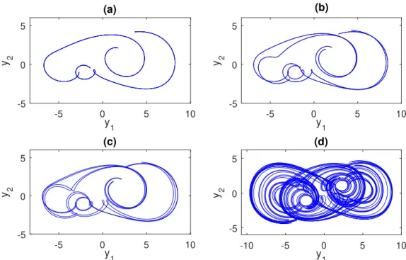
4 Period-doubling cascade
In this part of the paper, we suppose that there exists a function G : R×Rm×R → Rm satisfying the periodicity condition G(t+T,x,µ) = G(t,x,µ)for all t ∈ R, x ∈ Rm, µ ∈ R, whereµis a parameter, such that for some finite valueµ∞of the parameter the functionF(t,x) on the right-hand side of system (2.1) is equal toG(t,x,µ∞).
System (2.1) is said to admit a period-doubling cascade [9,14,22,36] if there exists a se- quence
µj , j∈N, of period-doubling bifurcation values with µj →µ∞ as j→∞ such that as the parameterµincreases or decreases throughµj the system
x0 =G(t,x,µ) (4.1)
undergoes a period-doubling bifurcation, i.e., there exists a natural number λ such that for eachj∈Na new periodic solution with periodλ2jTappears in the dynamics of system (4.1), and consequently, system (4.1) possesses infinitely many unstable periodic solutions all lying in a bounded region forµ=µ∞.
We say that the impulsive system (2.2) replicates the period-doubling cascade of system (2.1) if for each periodic solutionx(t)∈A of (2.1) system (2.2) admits a periodic solution with the same period.
Under the conditions (A1)–(A5), one can verify using the results of [4,35] that ifx(t)∈A is aλ0T-periodic solution of system (2.1) for some natural numberλ0, then the corresponding bounded solutionφx(t)(t)of (2.2) is alsoλ0T-periodic. Moreover, the instability of all periodic solutions of (2.2) is ensured by Theorem3.2. Therefore, we have the following theorem.
Theorem 4.1. Assume that the conditions (A1)–(A7) are valid. If system (2.1) admits a period- doubling cascade, then the impulsive system(2.2)replicates the period-doubling cascade of (2.1).
A corollary of Theorem (4.1) is as follows.
Corollary 4.2. Assume that the conditions (A1)–(A7) are valid. If system (2.1) admits a period- doubling cascade, then the same is true for the coupled system(2.1)–(2.2).
Remark 4.3. One can confirm that the sequence{µj}of period-doubling bifurcation parameter values is exactly the same for both system (2.1) and the coupled system (2.1)–(2.2). Therefore, if system (2.1) obeys the Feigenbaum universality [14], then the same is true also for the coupled system (2.1)–(2.2). More precisely, when limj→∞ µµj−µj+1
j+1−µj+2 is evaluated, the universal constant 4.6692016 . . . known as the Feigenbaum number is achieved, and this number is the same for both system (2.1) and the coupled system (2.1)–(2.2).
The next section is devoted to illustrative examples that support the theoretical results.
5 Examples
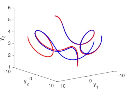
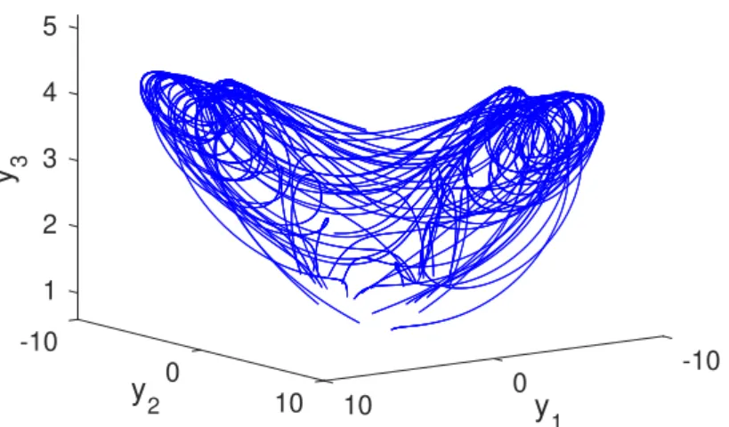
In this part of the paper, two examples will be presented. In the first example the replication of sensitivity in an impulsive system driven by a chaotic Lorenz system will be demonstrated numerically, whereas in the second one replication of period-doubling cascade in an impulsive system driven by a Duffing equation will be discussed.
5.1 Example 1
Let us consider the Lorenz system [25]
x01 =−10x1+10x2, x02 =−x1x3+28x1−x2, x03 =x1x2− 8
3x3.
(5.1)
It was demonstrated in [25,41] that system (5.1) is sensitive and it possesses a chaotic attractor.