Discrete mathematics

(1)

Discrete mathematics

Tibor Juhász

(2)

Discrete mathematics

Tibor Juhász

(3)

Preface

This volume of college notes aims to make the Discrete mathematics 1 lectures easier to follow for Eszterházy Károly College’s Software Information Technologist students. When structuring the material, we considered that the students attending this course already possess a higher knowledge of mathematics, because in the previous semester, within the frames of “Calculus 1” the basic set theory and function studies have been included, although the majority of the notes material can be understood with even a stable secondary school- level knowledge.

Actually, mathematics consists of creating concepts and detecting the logical bonds between these concepts.

Here, when defining a new concept, the concept itself is written in cursive. These definitions are as precise as the conditions allow them to be. In many cases the utterance of a statement takes place as part of the context, but in some cases it is highlighted as a theorem. Mathematical statements usually require demonstrations, although here – in regard to the target group’s needs, its preparedness, and the given time allowance – we do not always show the demonstrations.

The tasks at the end of each chapter help to measure the intensification of the discussed material: we suggest that the reader should not consider a chapter processed until he or she has any difficulty with the task at the end of it.

The aim of this notes is not to show the possible applications of mathematics in informatics, but merely to provide the appropriate mathematical basis necessary for this application.

(6)

(7)

Chapter 1. From the natural numbers to the real numbers

The first mathematical experiences of our lives are connected to the acquisition of numbers, even as toddlers we are capable of dealing with them. In spite of that, the precise mathematical establishment of the concept of numbers reaches beyond the level of elementary mathematics. Everybody has a stable notion of the meaning of

“two”, but many would be in trouble providing an exact definition. We cannot promise to give the exact construction of the concept of numbers within this notes, we merely attempt to picture its atmosphere in this chapter. Our aim is to summarize the characteristics of those significant sets of numbers known by us from secondary school, which are important for us.

1. Natural numbers

In childhood, the acquisition of numbers is a result of a certain abstraction: sensing the permanence of the cardinality of objects around us.

Figure 1.1. What is the same between these three sets?

The concept of “two” begins to loom as two biscuits, two building blocks, or a common feature of our two hands. This recognition is captured by the definition of natural numbers deriving from set theory, according to which, we consider the cardinality of finite sets as natural numbers. As it is well-known from “Calculus”, the empty set is finite, its cardinality is denoted by 0. The cardinality the set whose only element is the empty set is denoted by 1, and 2 is defined as the cardinality of the set , and so on. The set of natural numbers is therefore the set

Figure 1.2. Natural numbers on the number line

We know that the set of natural numbers is closed under addition and multiplication.

Figure 1.3. The sum and the product of two natural numbers are also natural numbers, but the same in not true for difference and quotient of natural numbers

(8)

From the natural numbers to the real numbers

This means that addition and multiplication assign to any two (distinct or equal) natural numbers a well-defined natural number. The following “good” properties of the natural numbers make the calculation much easier.

1.

Both addition and multiplication on the natural numbers are commutative, that is, changing the order of the summands or factors does not affect the result:

for natural numbers a and b.

(9)

2.

Both operation are associative, that is

for all . This property can be interpreted as follows: if we want to add three numbers and c together, it is the same that we add a and b first, then add c to the result, or we add b and c first, then add the result to a. As we can rearrange the parentheses without changing the result, the parentheses will be often left.

As we will see later, these two properties together guarantee that the sum and the product of finite many natural numbers are independent of the distribution of parentheses and the order of the terms and factors.

The next property describes a relationship of the two operations.

3.

Multiplication is distributive over addition, that is

for all natural numbers .

We raise the reader’s attention to 0’s relation to addition, and 1’s relation to multiplication: adding 0 to any number does not change the number, and any number remains unaltered when multiplied by 1.

With the aid of addition we can introduce an order on the natural numbers by letting (a is less than or equal to b), if there exists a natural number c with . Furthermore, (a is less than b), if , but . We will often use the fact that every nonempty subset of the natural numbers has a minimal element.

1.1. Induction

It is also clear that for any natural number n, is also a natural number. Moreover, if H is a subset of the natural numbers, which contains 0, and it contains whenever it contains n, then H contains all natural numbers. It is based on this assertion an important method of mathematical proof, the so-called induction, which is used to establish a given statement for natural numbers, and it consists of the following two steps:

1.

First we prove the statement for 0 (or for the first natural number for which the statement is relevant).

2.

Then we show that the given statement for any one natural number n implies the given statement for the next natural number . This is known as inductive step.

The two steps together ensure that the statement is true for all natural numbers: by the first step, it is true for 0, then by the second step, it is also true for 1, then applying the inductive step again we obtain the statement for 2, and so on. Demonstratively speaking, a man capable of stepping up the lowest step of a stairway, and of stepping onward to any further step of it, is sure to ascend the whole stairway.

As an example, we show that

for all natural number .

(10)

First we have to verify the case : the equality

is indeed true. Now, suppose the statement for some natural number , that is

and using this, we should conclude the statement for , that is

Applying the assumption (1.1) we have

It is easy to check that the right-hand side of (1.2) is equal to the same. As already explained above, this claim is proved. We emphasize once more that the equality (1.1) is only an assumption. If we were able to prove it directly, we would not need induction. Moreover, we could have even supposed the statement not only k, but all natural number that less than or equal to k. In this case we did not need for that, but it can happen that it is necessary to conclude the case (see e.g. Theorem1.2).

We will prove now that every horse has the same colour. We will do it by induction on the number of horses. If we have only one horse, the statement is evident. Suppose that the statement is true if we have k horses, and let us consider a group of horses. Let us number the horses in this group: . The horses of numbers and form groups of horses of sizek, and, by the inductive hypothesis, all the horses are the same colour in both groups. As the horse numbered 2 belongs to both group, so all the

horses are the same colour.

The statement we have just proved is definitely false. This so-called horse paradox does not want to be an attack against the induction, it just want to draw the reader’s attention for a possible error. The error is that the argument we used in the inductive step is only correct if k is at least 2, because there only then exists a common horse in the two groups of horses of size k. Therefore, the inductive step forces us to check the statement not only for , but for as well. However, nobody can state that two arbitrary horses are always one- coloured.

2. Integers

(11)

Those, who have peeped forward in the notes were able to see that sooner or later we will intend to solve equations. Within the set of natural numbers, even solving the equation is problematic, because there is no such natural number to which, if we add 1, we get 0, or to put it another way, we cannot subtract 1 from 0. An expansion of the set of natural numbers is therefore needed. We can reach that, if we regard the

symbol, where n is a natural number bigger than 0, – a number, and call it the negative of n. The set

Figure 1.4. Integers on the number line

is called the set of integers, and its elements are the integers. The expansion will be successful if we escalate the operations used with natural numbers to this new, expanded set. The escalation refers to the fact that the “new”

operation should produce the usual result on the “old” numbers. The success of this was visible for everybody in elementary school: the sum of integers 2 and 3 will be 5, the same way as they would have been added as natural numbers. Moreover, the good qualities of addition and multiplication: commutativity and associativity also remain. The profit of the expansion is that for every x integer, another integer can be found (this, we call the opposite of x), so that the sum of these two is exactly 0. Thus, we can state that within the set of natural numbers, substraction can also be done, because substraction is nothing else but addition with the opposite.

We can extend the order to the integers as well: we say that , if is a natural number. If , then a is said to be positive, and if , then a is called negative.

As it is well-known, we cannot divide any two integers by each other, for example, the quotient of 12 and 5 is not an integer. However, there is a conventional process of division of two integers, which produces a quotient and a remainder.

Theorem 1.1 (The division algorithm). For any integers a and bwith , there exist

unique integers q and r such that and .

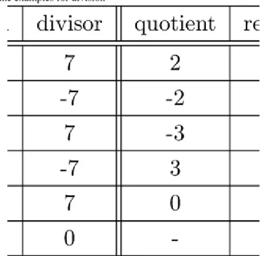
Before the proof we mention that we will refer to a as dividend, b as divisor, q as quotient, and r as reminder.

The restriction for the reminder is needed because of the uniqueness. Without that, we can say that “dividing 20 by 7 results 1 as quotient, and 13 as remainder”.

Proof. Let us consider the integers

which is the sequence of integers of the form with , extending indefinitely in both directions. Amongst them there definitely exists a smallest non-negative, let us denote it by r. Then for some integer k; let . Hence, . We show that . Indeed, in the contrary

were true, which would lead to when b is negative, and to otherwise. This contradicts to the fact that is the smallest non-negative integer from the sequence above.

Now, suppose that are integers such that

and

(12)

By subtracting the first equation from the second one and rearranging, we get the equality

Let us take the absolute values of both side (factor by factor on the left-hand side):

By the assumptions for and , the right-hand side of this equality is less than . The same can only be true for the left-hand side if . But then the left-hand side is zero, so should the right-hand side too , thus , which means that q and r are uniquely determined.

Figure 1.5 shows some examples for division.

Figure 1.5. Some examples for division

We note that to the remainder r alternative restrictions can be given instead of , so that the uniqueness of q and r remains intact. For instance, we may also consider as the possible remainders of the division by 5 the elements of the set . Recall that we make a repeated application of the division algorithm for converting integers between different numeral systems.

2.1. Divisibility

We first clear the concept of divisibility. Let a and b integers. We say that a is divisible by b (or: b is a divisor of a, or: a is a multiple of b), if there exists an integer c such that . In notation: .

The next statements follow directly from the definition.

1.

Zero is divisible by every integer.

2.

Zero divides only itself.

3.

(13)

Every integer is divisible by and 1. The integers and 1 are called the unitsof the integers.

4.

If and , then or .

And some relationships between the divisibility and the operations of the integers:

5.

If and , then .

6.

if and , then .

As an example, we prove the statement 5. If and , then by the definition of divisibility there exist

integers k and l such that and . Then , whence, being

integer, follows. The other statements can be proved similarly.

We continue with the concept of the greatest common divisor. The integer d is said to be a common divisor of the integers a and b, if d divides both a and b. It is easy to check that if and , then , which implies that every nonzero integer has only finite number of divisors. So, if at least one of a and b is not zero, then they have finite number of common divisors, and then amongst these common divisors there is a greatest one. Even though we define the concept of the greatest common divisor in another way: the integer d is called thegreatest common divisor of the integers a and b, if d is a common divisor of a and b, and every common divisor of a and b divides d. For example the common divisors of 28 and 12 are , amongst them and 4 divides any one, so they are the greatest common divisors.

We prove first that if the integers a and b have a greatest common divisor, then it is unique up to the sign. This is because if and are greatest common divisors, then , on the other hand, ; that is

or . Furthermore, if d is a greatest common divisor of a and b, then so is . The non-

negative between them will be denoted by . Therefore, .

Now, we show that any two integers have greatest common divisor, and that how to find it. Let a and b be integers with . If , then it is clear that . Otherwise, by the division algorithm, a can be expressed as

where . If is not 0, then we repeat the division algorithm: the dividend and the divisor in the next step is always the divisor and the remainder from the previous step:

(14)

where . Since the remainders get smaller and smaller, they have to attain 0:

and at this point the algorithm stops. This method is known as Euclidean algorithm on the integers a and b, and the integer is called the last nonzero remainder in the Euclidean algorithm. We state that is a greatest common divisor of a and b. Indeed, climbing up the equalities(1.3)-(1.7) from the bottom to the top, we obtain

that is, is a common divisor of a and b. But if d is also a common divisor, then the same equalities looking from the reverse direction (from up to down) give that . Thus is a greatest common divisor.

2.2. Primes

As we know from earlier, the primes are the integers whose have exactly two positive divisors. Evidently, this two divisors are 1 and the absolute value the number. By this definition, none of the integers is prime, because 0 has infinite number of positive divisors, whereas the other two have only one. The following statements give us a fair show to characterize the primes in other ways.

1.

An integer other than 0 and is prime if and only if it can only be written as a product of two integers that one of the factors is or 1.

2.

An integer other than 0 and is prime if and only if implies or .

The second statement can be expressed as a prime can only divide a product, if it divides one of the factors of the product. For example, 6 is not prime, because but 6 does not divide either 2 or 15.

The next theorem shows that the primes can be considered as the building blocks of the integers.

Theorem 1.2 (The fundamental theorem of arithmetic). Every integer other than 0 and is a product of finite number of primes (with perhaps only one factor) in one and only one way, except for the signs and the order of the factors.

So, the prime factorizations , , and of 10 are essentially the same.

Proof. We first prove the theorem for natural numbers: we are going to show that every natural number greater than 1 can be uniquely (in the above sense) expressed as a product of finite many primes. We use induction: let first . Since 2 is prime, so we can consider it as a product with a single factor. Assume the statement for all natural numbers from 2 tok. We are going to show that the statement is true for as well. This is obvious if is prime. Otherwise, there exist natural numbers and such that , and . By the inductive hypothesis, and can both be written as product of finite number of primes, and so is .

In order to prove the uniqueness, assume that the natural number is the product of prime numbers in two different ways:

(15)

and suppose that . Then , and as is prime, divides any factor of the product ; say . Since is prime, too, so , and from (1.8) it follows that

Repeating the same kind of argument, we are step by step led to , and finally we arrive at the equality

Since 1 cannot be a product of primes, so the primes on the right-hand side cannot “exist”, therefore . This means that there cannot be two essentially different factorizations.

It remaind the case when when n is an integer less than . Then is a natural number greater than 1, so, as we have seen before, is a product of finitely many positive primes:

. Then is a possible prime factorization.

Furthermore, ifn had two prime factorization differ not only in the order and signs of the prime factors, then would have two prime factorization like that, which contradicts to the above-mentioned conclusion.

Let us mention that for , in the expression the primes are not necessarily distinct. By collecting the same primes together, n can be written in the form

where are distinct primes and are positive integers. This representation of n is called the canonical factoring of n.

It is clear that if and , then the canonical factoring of d is of the form

where . In other words, a prime occurs in the canonical

factoring of d only if it also occurs in the canonical factoring of n, and its exponent is certainly not greater. The converse is also true: every natural number of canonical factoring like that divides n. As a consequence, for and , can be determined by writing the prime factorizations of the two numbers as follows: take all common prime factors with their the smallest exponent and multiply them together. For instance, and . The common prime factors are 2 and 7, the least exponent for 2

is 2, for 7 is 1, so =28.

It also follows from the fundamental theorem of arithmetic that every integer different form 0 and is divisible by a prime.

Once prime numbers possess such an important role, let us observe some statements referring to them. We show first that the number of primes is infinite. Indeed, if we had only finite number of primes, and say, were the all, then let us see what about the integer . According to fundamental theorem of arithmetic, N can be written as a product of primes. Since N is not divisible by

, there must exists primes distinct from , which is a contradiction.

(16)

If we would like to decide that whether a natural number is a prime or not, it is enough to investigate if if has any positive divisor different from itself and 1 or not. Let pbe the least positive divisor of n. Then for some integer c. As c is also a divisor of n, so , and . Hence

, which means that the least positive divisor different form 1 of cannot be grater than . For example, in order to observe if 1007 is a prime or not, it is enough to look for positive divisors up to

. Moreover, it sufficient to search amongst the primes, so we must verify the divisibility of 1007 by only the primes 3, 5, 7, 11, 13, 17, 19, 23, 29 and 31. By checking one and all it turns out that 19 divides 1007, so 1007 is not prime.

Finally, we can see an algorithm for finding all prime numbers up to any given limit. Create a list of integers from 2 to n:

We frame the first number of the list and cross out all its multiples:

The next unframed and uncrossed number on the list is the 3, we frame it and cross out all its multiples (some of them may have already been crossed out, in this case there is no need for crossing out it again):

The method continues the same way: the first uncrossed and unframed number gets framed, and its multiples get crossed. About the framed numbers it can be stated, that they cannot be divided by any number which is smaller than them and bigger than 1, namely, a prime. The crossed numbers are the multiples of the framed ones, so they cannot be primes. This algorithm is known as the Sieve of Eratosthenes. It also follows from the above- mentioned facts that if we have already framed all primes up to , then every unmarked element of the original list will be prime.

Figure 1.6. The list of primes below 100

(17)

3. Rational numbers

Although, we have told quite a few things about integers, but even a very simple equation like

cannot be solved with them. It is clear, because here we need a number, which, if we multiply it by 2, we get 1, but such an integer does not exist. Yet again we have to do some construction, sticking to our set rules. By a fraction we mean a symbol , where a and b are integers with . Furthermore, the integers a and b are called the numerator and thedenominator of the fraction. The fractions and are said to be equals if

. For example,

It is also follows that multiplying both the numerator and denominator of a fraction by the same nonzero integer results a fraction that is equal to the original one. The fraction is called simple fraction, if . Every fraction is equal to exactly one simple fraction with positive denominator. The set of all fractions is said to be the set of rational numbers, and it is denoted by .

The addition and multiplication on the set of rational numbers are defined as follows:

(18)

We remark that in the above formula the symbols on the left and right-hand sides have a different meanings.

On the left hand side it denotes the addition of rational numbers which is just being defined by this formula, whereas on the right-hand side the stands in a numerator of a fraction, so it means the addition of integers.

We may say the same about the sign of the multiplication in the second formula.

Obviously, we would like these operations to possess all the properties that we are familiar with: both the addition and multiplication should be commutative and associative. It is easy to see that they all hold, as an example, we verify the associativity:

and

Both equalities led to the same formula, so the formulas on the left-hand sides have to be equal, the addition of the fractions is therefore associative. We should notice that, in the meanwhile, we have made use of nearly all the previously mentioned properties of addition and multiplication of integers in the numerator.

We can prove similarly that multiplication is distributive over addition.

But how does the set of natural numbers become the extension of the set of integers? How can we spot integers among rational numbers? The answer is simple: we make the fraction correspond the integer a. This is a one- to-one correspondence between the set of integers and the subset

of rational numbers. Furthermore, if we add or multiply together the rational and instead of the integers a and b assigned to them, then the sum and the product are and , which are exactly corresponded to the integers and . This means that if we add or multiply integers as rational numbers, the result will be the same as if we had done the same with them as integers. In view of that, we can simply write a instead of the fraction .

It is also true that the 0 (or the fraction ) does not change any number when we add it to them. Furthermore, adding the fraction to the result is 0, so every rational number has an opposite. The existence of the opposite enables the substraction as addition with the opposite. It is easy to see that multiplying the fraction by any other fraction, the latter will not change, so the 1 as a rational behaves with regard to the multiplication as it does within the integers. But within the integers 1 can be divided only by itself and , all fraction other than divides , in other words, for every fraction there exists a fraction, namely , such that their product is equal to 1. The fraction is said to be the reciprocal of . If we consider the multiplication by the

(19)

reciprocal as division, then we can state that every rational number can be divided by every nonzero rational number, and the result will also be a rational number.

So, we can say that within the rational numbers the addition, subtraction and multiplication can be performed without restraint, moreover even the division, under the restriction that division by zero is not defined.

Finally we draw the attention to another property of the rational numbers, which does not hold for integers:

between two arbitrary (distinct) rational numbers there is a third rational numbers. Indeed, let and be rational numbers, and assume that . Then their arithmetic mean

is also a rational number, furthermore

Figure 1.7. The middle points given by the repeated bisection of the interval seemingly cover the whole interval

In view of this property we say that the set of rational numbers is dense, for every point x of the number line you can find a point belonging to a rational number that are as close as you want to x. But this does not mean that every point of the number line corresponds to a rational number. We know from secondary school that the number corresponding to the length of the diagonal of the unit square is not rational.

4. The real numbers

Returning to the solvability of equations, we can state that all the equations of the form , where a and b are rational numbers, and are solvable within the rational numbers, and the only solution is . The situation is different if the square of the unknown also occurs: as it is well-known, the equation has no solution in the set of rational numbers. Let us take a point of the number line. It can happen that this point corresponds to a rational number. If not, we will take the distance of this point from the point 0 (with sign), and consider it as a number. If we extend the set of rational numbers with these numbers, we get to the so-called real numbers, in which the above equation has two solutions: and . Within the real numbers the four elementary operations can be performed unrestrictedly (apart from division by zero), and every non-negative real number has a square root. However, the negative numbers has no square roots, so, for example, the equation is not solvable even in the real numbers.

Figure 1.8. There is a one-to-one correspondence between real numbers and the point of the number line

(20)

5. Exercises

Exercise 1.1. Prove that

a.

the sum of the first n positive integers is ; b.

the sum of the first n odd natural numbers is ; c.

the sum of the cube of the first n positive integers is

holds for any natural numbers .

Exercise 1.3. Recall the concept of order relation from Calculus, and prove that the division ( ) is a partial order on the integers.

Exercise 1.4. Apply the division algorithm on the integers and in all the possible ways.

Exercise 1.5. What is Exercise 1.6.

Execute the Euclidean algorithm on and , and find the greatest common divisors of a and b.

(21)

Exercise 1.8. When is the sum of the positive divisors of a positive integer even or odd?

Exercise 1.9. The difference between two positive primes is 2001. How many positive divisors has the sum of these primes got?

(22)

Chapter 2. Complex numbers

Our goal is to construct a set of numbers which satisfies the following requirements:

• it is closed with respect to the four elementary arithmetic operations, and the well-known arithmetical laws remain valid;

• it contains the set of real numbers in such a way that elementary arithmetic operations on the reals work the same as we are used to;

• its every element has a square root.

As there is a one-to-one correspondence between the real numbers and the points of the number line, it is not possible to extend the numbers in one-dimensional.

1. Operations on points in the plane

Let us consider the set of all points of the plane , and introduce the

addition and multiplication on it as follows:

Then is closed under these operations, that is the sum and the product of points in the plain are points in the plane as well. Both operations are commutative and associative, that is the properties

hold for any . The addition inherits these features from real numbers, because when adding complex numbers, virtually we add real numbers in both coordinates. We demonstrate the associative property of multiplication, and after that, checking the commutativity is not problematic at all. Let

and . Calculating the products and (and using

that the addition of real numbers is commutative) we can see that both products lead the same result:

and

The reader can easily verify that the distributive law also holds, that is for all points and w.

The origin is the point which, when being added to any other point, does not change that, this is the so-called additive identity of . Furthermore, for any point there exist a point, namely , such that the sum of them is exactly the additive identity, in other words, every point has an opposite (or additive inverse).

Thanks to that, substraction, as addition with the opposite, can arbitrarily be done at any points of the plain.

When is multiplied by any point in the plane, yields , so is the so-called unity (or multiplicative identity). Now, we prove that every point other than the origin has a reciprocal (or

(23)

Complex numbers

multiplicative inverse), that is, there exists a point by which multiplied results . Indeed,

performing the multiplication in the equality we have

. Since two ordered pairs are equal exactly when their first elements are equal and their second elements are equal, so we get the system of equations

It is easy to read the solution when one of a and b is zero. Otherwise we can multiply the first equation by aand the second one by b to get

then by adding the two equations together we have . Hence,

If in (2.1) we multiply the first equation by b, and the second one by a, then, we get as before that

To sum up, the reciprocal of the point other than the origin is

The existence of reciprocal ensures the possibility of division. So, our first requirement holds entirely.

The set of all ordered pairs of real numbers with the addition and multiplication introduced above is called the set of complex numbers, and it is denoted by . The first component of the complex number is said to be the real part of z, and its second component is the imaginary part of z. In notation: , and

.

Let us consider the subset of the complex numbers. The sum and product of two elements of R is also an element of R:

Regarding the first components (which are obviously real numbers) we can argue that in R the operations

“function” the way we know it from the set of real numbers. Furthermore, the mapping , is a one-to-one correspondence between the real numbers and the elements of R, so the elements of R can be identified with the real numbers.

Figure 2.1. Numbers

(24)

Complex numbers

The proof of the holding of our third requirement will be done later, but we can already tell that for example the opposite is the unity, which is (it has just identified with ), will be a square of a complex number:

We will denote this complex number by i, furthermore – motivated by the above-mentioned identification – we will simply write a instead of . Then the complex number , by the decomposition

can be written in the form , which is the usual notation of complex numbers.

2. Elementary operations on complex numbers

Using the usual notation of complex numbers we can perform the addition, subtraction and multiplication as we usually do with sums of more than two terms, keeping in mind that :

and

For the sake of demonstrating here are a few examples:

(25)

Complex numbers

Before we turn to the division we define the conjugate of the complex number as .

For example, . It is easy to check that the

following properties hold for any complex numbers z and w:

• if and only if z is a real number;

• ;

• if , then .

In order to divide the complex number by the nonzero complex number we multiply both the nominator and denominator of the fraction by the conjugate of the denominator. Then the fraction will not change, and

Let us observe this with concrete complex numbers, then compare the result with the examples from the multiplication:

For exponentiation and computing the nth roots the usual notation of complex numbers is hardly usable.

3. Polar coordinates of complex numbers

It is clear that the point in the plan, or, in other words, the complex number in the Cartesian coordinate system can be characterized by the distance of the point form the origin, and by the angle between the line joining the point to the origin and the positive x-axis. This angle is called the argument of

. For example, the argument of is , and the argument of is . In general, to determine the argument of a complex number we need to solve the equation , provided that . Keeping in mind that the period of the tangent function is 180 degrees, so the above equation has infinitely many solution; to choose the argument amongst them it is enough to know which quarter plane contains the complex number.

Figure 2.2. Complex numbers on the plane

(26)

Complex numbers

If we are brave enough to calculate in radians, then we can determine the argument by the aid of the inverse function of the tangent as follows:

Figure 2.3. The graph of the function

Figure 2.4. The graph of the function

(27)

Complex numbers

By the Pythagorean theorem, the distance of the point from the origin is ; this non-negative real number is called the absolute value of the complex number . This notion is synchronized with the absolute value known from the set of real numbers, and the following properties hold for any :

• ;

• .

It is obvious that two complex number given by their absolute values and arguments are equal if and only if the absolute values are equal and the difference of the arguments is a multiple of 360 degrees. Furthermore, if is a complex number with absolute value r and argument , then by Figure 2.2,

and , therefore

The formula on the right-hand side is the representation in polar coordinates of the complex number . The complex number 0 has no such representation.

As an example, we write the polar coordinate representation of the complex number . Then , and the argument can easily read if we draw the point into the Cartesian coordinate system: . So, the polar coordinate representation is

. Let now . Then

. In order to determine the argument we solve the equation . Hence , where k is an arbitrary integer. Regarding as z is in the second quarter plane, , thus , and the polar coordinate representation of z is:

.

Figure 2.5. The argument of the complex number

(28)

Complex numbers

4. Operations with complex numbers in polar coordinates

Using polar coordinates makes the calculation with complex numbers more simple. Let and be complex numbers. After recalling the angle addition formulas

and

it is easy to check that

that is the products of two complex numbers are therefore obtained by multiplying their absolute values, and adding their arguments. Since the exponentiation on positive integers is repeated multiplication, the nth power of the complex number , where n is a positive integer, is

(29)

Complex numbers

This formula is known as Moivre’s formula, and is says that positive integer powers of a complex number can be obtained by rising the absolute value to the given exponent, and multiplying the argument by the exponent.

As an example, we compute the tenth power of . In order to use the Moivre’s formula, we have to convert

the complex number to polar coordinate representation: . Hence

Because the exercise is posed in usual notation, we have converted the result to usual notation from polar coordinate representation. It is easy to see that the reciprocal of the complex number

is

because . Using the multiplication and the reciprocal, the quotients of the

complex numbers and can be obtained as follows:

In other words, the quotients of two complex numbers can be get by dividing their absolute values and subtracting their arguments. Thus, Moivre’s formula is valid for arbitrary integer, and the well-known exponentiation identities hold.

5. nth root

We are able to fully reach our target if we show that for any positive integer n there exists nth roots of any complex number. To this we first clear what we mean by an nth root of a complex number. Let n be a positive integer. By the nth roots of the complex number z we mean all complex numbers whose nth power is z. Pay attention! In our previous study the square root of 9 was only 3, but now the definition is satisfied by not only 3, but also . So, the nth root of the complex number z is usually not a single complex number, but rather a set of complex numbers. In order to avoid the confusions, the radical symbol will only be used for the nth roots of real numbers.

Let be an arbitrary nonzero complex number, and let us look for the nth roots of z in polar coordinate representation. If is an nth root of z, then . We can apply the Moivre’s formula to have

On both sides of the equality there are complex numbers in polar coordinate representation, so the equality holds only if

(30)

Complex numbers

for some integer k. The unknown in the first equation is an absolute value of a complex number (that is, a real number), so we have to solve that over the real numbers: the only solution is . From the second equation follows. The nth root of the complex number z is therefore the complex numbers

where . Does it mean that every complex number has infinitely many nth roots? On trial determine the third (or cube) roots of . The polar coordinate representation of is . Our formula gives the following result for :

Going on with the case we have , which is the same as

we obtained for .

Let u and v be arbitrary integers, and divide the integer by n: , where q and t are

integers, and . Then

This shows that the difference between the angles and is a multiple of 360 degrees only if , that is the complex numbers given by the formula (2.2) are equal for and if and only if

is divisible by n. So, applying the formula(2.2) for we obtain n distinct complex numbers, and there is no other value of (2.2) for any other k. This means that every nonzero complex number has precisely n distinct nth roots.

Turning back to the example, has exactly 3 different third roots, namely and . Furthermore, we can state that the set of complex numbers is closed under the “extraction of roots” operation, so all of the initial requirements are satisfied.

The 1 is a complex number too, so it also has n distinct nth root, they are called the nth roots of unity. The determination of the roots of unity can also happen by the formula (2.2). As the polar coordinate representation of 1 is (we left the factor ), by (2.2) the nth roots of unity are:

where . For example, the fourth roots of unity are:

(31)

Complex numbers

Figure 2.6. Fourth roots of unity

A N I M A T I O N

It is evident that is always 1, and it is not so hard to see that, all the nth roots of unity can be obtained by rising to the exponents . Taking the above example, the fourth roots of unity can be

obtained as the powers of i, namely: and .

If we have the nth roots of unity, the extraction of nth roots is easier to done: if w is an nth root of the complex number z, then all the nth roots of z are precisely

that is it is enough to multiply w by all the nth roots of unity. The proof is left to the reader.

(32)

Complex numbers

Applying this statement we compute the fourth roots of . Using the

formula (2.2) with , we have that is one of the fourth roots.

Recalling the fourth roots of unity, the other three are the following: ,

that is and .

Finally, we remark that the well-known identities for nth roots from the secondary school cannot in general be extended to complex numbers.

6. Exercises

Exercise 2.1. Fill the following table.

Exercise 2.2. Where are on the plane the complex numbers for which

1.

; 2.

; 3.

?

(33)

Complex numbers

Exercise 2.3. Give the value of and . What is equal to? What is equal to, if n is an arbitrary integer?

Exercise 2.4. Express the complex number

in the form .

Exercise 2.5. Let and . Write the expression

in the form !

Exercise 2.6. Represent the complex numbers

in polar coordinates.

Exercise 2.7. Write the complex number

in the usual notation.

Exercise 2.8. Simplify the following expression:

Exercise 2.9. Determine the second and third roots of unity.

Exercise 2.10. Compute the eighth power and the third roots of the complex number .

Exercise 2.11. Let a be an arbitrary real number. Give the square roots of a.

Exercise 2.12. Give the square roots of and .

Exercise 2.13. Given the square roots of and without using polar coordinates. (Hint: find the square roots of in the form ; then

.)

Exercise 2.14. Solve the equations

and

over the set of complex numbers.

(34)

Chapter 3. Polynomials

Let F be the reader’s favourite among the sets of rational, real, or complex numbers. Let us consider the elements of F, the so-called undetermined x, and see what expressions can be produced out of these by addition and multiplication in finitely many steps. It is easily detectable that these expressions might contain any non- negative exponent power of x, any product of these by elements of F, or the sum of all these. In other words, after expanding the parenthesis, rearranging, and combining of like terms, we get to an expression in the form

where belong to F, and n is a natural number. This formal expression is called a polynomial over F, and the numbers are the coefficients of the polynomial. The expression is said to be thejth-degree term of the polynomial. In notation we may write f instead of , as long as we do not want to emphasize that x is the indeterminate. The complexity of the formula defining a polynomial is caused by the fact that we cannot de facto perform the multiplication of the undetermined x by an element of F, so for instance we can handle the double of x only formally, as 2x, moreover, we can only formally add terms of different degrees together. We only assume about x, that what is valid for every element of F, is also valid for x, so, for instance: . Consequently, , so we usually omit terms like these. For example, in the formula (3.1) there is no term of degree greater than n, so their coefficients are considered to be zero. A polynomial has therefore only finitely many term with coefficients other than zero. According to the definition, it can happen that all the coefficients are zero; this polynomial is called the zero polynomial and it is denoted by 0.

If , look for the largest integer k for which . This number kis called the degree of the polynomialf , and it is denoted by . The degree of the zero polynomial is undefined. In order not to regard the zero polynomial as a constant exception, we regard the degree of the zero polynomial as existing, and as less than the degrees of any other polynomials: let the degree of the zero polynomial is .

We will denote by the set of all polynomials over F.

Two polynomial are considered to be equal, if the sequences of their coefficients are equal, that is, for any the coefficients of in the two polynomials coincide. Evidently, equal polynomials have the same degree.

1. Operations with polynomials

We can introduce addition and multiplication on the set of all polynomials over F as follows. Polynomials can be added by adding the coefficients of the terms of the same degree, and they can be multiplied by multiplying every term by every term so that the product of the terms and is , then we add the terms of same degree and rearrange the terms so that the power of x are in ascending order. For example, let

and . Then

and

About the degrees of the sum and product polynomials we can say the following: the degree of the sum polynomial cannot be greater than the degrees of the summands, that is

(35)

Polynomials

The equality holds exactly when f and g are of the same degree, and the sum of the coefficient of their terms of highest degree is zero. Furthermore,

that is the degree of the product polynomial is always equal to the sum of the degrees of the factors. Here we used that a product of elements of F can only be zero if one of the factors is zero. The truth of this statement for complex numbers will be proved later, under more general conditions.

The addition of the polynomial is commutative, associative, its additive identity is the zero polynomial, furthermore, every polynomial f has an opposite, namely the polynomial , whose coefficients are the opposites of the coefficients of f . Therefore, the set of all polynomials is closed under substraction, which means adding the opposite. The properties of commutativity and associativity hold for the multiplication of polynomials as well, the unity is the polynomial . None of polynomials of degree at least 1 has reciprocal, because by multiplying polynomials their degrees are added together, so a polynomial multiplied by a polynomial of degree at least 1 cannot result the polynomial of degree 0. Therefore, only the polynomials of degree zero have reciprocal, and they indeed have, because they are exactly the elements of F other than 0.

Because of the lack of reciprocal, we can only make the division as we have seen at the integers.

Theorem 3.1 (Division algorithm for polynomials). Let f and g be polynomials over F, such that . Then there exist unique polynomials q and r over F, such that

, and the degree of r is less than the degree of g.

Proof. We start with the proof of the uniqueness, that is we are going to show that there is only one pair of polynomials satisfying the conclusion of the theorem. Assume the contrary: there exist polynomials and such that

where and are less than , and . Subtracting the second equality form the first one, after rearranging we have the equality

Since , the degree of the polynomial on the left-hand side is at least than , whereas the degree of the polynomial on the right-hand side is less than the degree of g, which is a contradiction. Thus, , and so the polynomial on the left-hand side of (3.2) is zero. But then also has to be zero, whence .

Now we show how to construct the polynomials q and r. Let

and

(36)

Polynomials

be polynomials of degree n and m, respectively. If , then by and the theorem is satisfied: . In the case when , divide the term of highest degree of f by the term of highest degree of g, and then multiply the quotient

by g, finally subtract this product from f . Denote by this difference:

It is clear that after subtraction the term of highest degree of f falls out, so the degree of will be less than the degree of f . If , the we can stop: and

. Otherwise, we repeat the method with the polynomial instead of f : we construct

the polynomial , for which . If ,

the we stop, otherwise we repeat again, using instead of . Since the degrees of the polynomials get smaller and smaller, after finitely many steps (say at the kth step) we get to the case when holds. It is easy to see that

thus the division theorem of the polynomials is true.

The polynomials q and r are called the quotient and remainder of the division of f byg.

The demonstration may become easier to understand through a concrete example. Divide the polynomial by . First we divide the term of the highest degree of f by the term of the highest degree of g: , we write this quotient to the right-hand side of the equality:

We multiply g by the quotient just obtained (by ), and we write the product under f :

We subtract the product just obtained from f , and write the result under a line:

The degree of the polynomial under the line is not less than the degree of g, so considering it as , we repeat the previous steps. The quotient of the terms of the highest degree of andg is , this will be added to the polynomial on the right-hand side of the equality, then we write the product of g and under

, which finally will be subtracted form :

(37)

Polynomials

Following the notations of the proof, the degree of the undermost polynomial is less than the degree of g, so the

procedure is done. The result is: and . We may verify ourself by

checking the equality

2. Polynomial evaluation

Let be a polynomial over F, and let t is a given element

of F. The element

of Fis called the value of at t. We emphasize that the expression above is not a formal expression any more, here we can evaluate the operations. We can put each element of F into the polynomial f , which leads to the mapping , which is called thepolynomial function of f . From the practical point of view there is no crucial distinction between a polynomial (as a formal sum) and the polynomial function attached to it, but later we will see that if we do not take the coefficients of the polynomials from the set of complex numbers, it can happen, that certain polynomial functions belonging to non-equal polynomials are equal.

Figure 3.1. The graph of the polynomial function of the polynomial of real coefficients, which have to be familiar from secondary school

There is an efficient method for evaluating polynomials, the so-called Horner’s method, which based on the fact that by factoring out x from the terms of degree at least 1, the polynomial

can be written in the form

(38)

Polynomials

and by factoring out x iteratively, we have

Substitute t for x into this expression. In order to evaluate the expression on the right-hand side we create a table as follows:

• in the first row we list the coefficients of the polynomial f , written in the descending order of the powers of x;

• in the head of the second row we write the x-value, then we copy the coefficients of the term of the highest degree under itself;

• the other entries in the second row are calculated for left to right by adding the coefficient above to the product of the x-value with the entry immediately to the left.

Let the entries of the second row be respectively. It is easy to see that

Then by (3.3), , that is the last entry of the second row is exactly the value of the polynomial f at t.

For example, Figure 3.2 shows the evaluation of for :

Figure 3.2. The Horner table for evaluation of the polynomial for

Thus . We can see that to determine we have needed 4 multiplications and 4 additions altogether. Without the Horner’s method the evaluation of the term would require 5 multiplications.

Another benefit of Horner’s method is the following: if we divide the polynomial f by the polynomial of degree one, then the coefficients of the quotient will be the numbers from the second row of the table, and is the remainder, that is

Returning to the example,

(39)

Polynomials

which is easy to verify.

3. Roots of polynomials

We will say that is a root of the polynomial , if . Here F plays a more important role than before. For example, the polynomial can be considered over or . In the first case f has no root, because there is no a real number t such that , whereas in the second case, the roots of f are the complex numbers i and .

In view of (3.4), if t is a root of the polynomial f , then f can be written as

where q is a polynomial over F of degree less by one than the degree of f .

Assume that the polynomial has a factor, that is, there exist polynomials and over F such

that . If t is a root of the polynomial f , then . Since a product of

elements of F can only be zero, if one of its factors is zero, it follows that or ; that is, t is a root of the polynomial f if and only if it is a root of g or h (or both).

Let be a root of the nonzero polynomial f , and let . If has a root, say , then we can factor out the polynomial from to obtain

where the degree of is less by 2 that the degree of f . We can continue the method for the polynomial provided that it has a root. As the degrees of the polynomials get smaller and smaller, sooner or later we get to the expression

where has no root. Evidently, then are the all roots of f , and by comparing the degrees of the polynomials on the two sides, we have . Therefore, the next statement is true.

Theorem 3.2. The number of the roots of a nonzero polynomial is not greater that the degree of the polynomial.

For the sake of completeness we remark that every element of F is considered as a root of the zero polynomial.

Theorem 3.3. If two polynomials of degree at most n have the same values at more than ndifferent points, then the two polynomials are equal.

Proof. If the polynomials f and g have the same value at the point b, then , that is . This latter means that b is a root of the polynomial . If the values of f and g were the same at more than n points, that would mean that has more than n different roots. As f and g are polynomials of degree at most n, then so is , and by the previous theorem, can only have roots more than n, if is the zero polynomial, that is .

(40)

Polynomials

From the theorem it follows that every polynomial of degree at most n can be uniquely given by its values at distinct points. The method how to find the polynomial given in this wise, the subject Numerical methods will tell more.

4. Exercises

Exercise 3.1. Give two polynomials of degree 4 whose sum is of degree 2.

Exercise 3.2. Divide f by g, where

a.

and ,

b.

and .

Exercise 3.3. Check by using the Horner’s method that, if the is a root of

. If it is, factor out the polynomial from f . Exercise 3.4. Make the division

using the Horner’s method.

Exercise 3.5. Find c such that the value of for to be 3.

Exercise 3.6. In general, how many addition and multiplication we need to compute the value of a polynomial of degree n at a given point, if we do it by Horner’s method?

Exercise 3.7. Give a polynomial of degree 3 whose all roots are: 1, 2 and i.

(41)

Chapter 4. Algebraic equations

By an equation we mean an expression , where F and G are a sort of functions of x, and by its solution set the set of all t’s from the intersection of the domains of the functions F and G for which the equality holds. The elements of the solution set are called the solutions. If the solution sets of two equations coincide, the two equations are said to beequivalent. The operations that transform a given equation into an equivalent one are called equivalent operations. The usual way of finding the solutions for an equation is that with the help of repetitive equivalent transformations we reduce the equation to such an equation which is way less difficult to solve.

Here we only deal with the case when both and are polynomials (more precisely, polynomial functions) with complex coefficients. Then multiplying both sides of the equation by the same nonzero complex number, and adding the same polynomial to both sides are equivalent operations. With the help of the latter we

can reduce the equation to , where is the polynomial , of

course. If f is polynomial of degree at least 1 over , then the equation is called algebraic equation. By the degree of the algebraic equation we mean the degree of the polynomial f . It is clear that the complex number t is a solution of the equation if and only if t is a root of the polynomial f , that is

. Because of this, the solutions of an equations are often called theroots of the equation as well.

The next theorem guarantees that every algebraic equation has a complex solution.

Theorem 4.1 (The fundamental theorem of algebra). Every polynomial of degree at least one with complex coefficients has at least one (complex) root.

By the theorem and (3.5), the polynomial

of degree at least one with complex coefficients can be written as

where the complex numbers are the roots of f . This form of the polynomial f is known as its linear factored form. It is also obvious that are solutions of the equation , and by Theorem3.2, there is no other solution. Of course, the numbers are not necessarily pairwise distinct, which means that we can only state that the cardinality of the solution set of an algebraic equation cannot exceed the degree of the equation. However, every polynomial of degree at least one can be written as a product of (not necessarily distinct) polynomial of degree one with factors as many as its degree.

Expanding the parenthesis in the product , we get a polynomial

where

(42)

Algebraic equations

Expressing in words, we obtain the number by choosing k-amount of roots out of in all the possible ways, and multiplying them together, then we add the obtained products. Comparing the coefficients of the polynomials, we have that

These formulae are known as Viete’s formulas, which relate the coefficients of a polynomial to sums and products of its roots.

For example, if the solutions of the quadratic equation are and , then the Viete’s formulas yield

which are well-known from the secondary school.

1. Solving equations in radicals

In the sequel we investigate how can we find all solutions of a general algebraic equation. By solving an algebraic equation in radical we mean a method which gives all solution of the equation by starting with the coefficients of the equation and rational constants, and repeatedly forming sums, differences, products, quotients, and radicals (n-th roots, for some positive integer n) of previously obtained numbers. For example, the only solution of the linear equation can be obtained by the help of division:

1.1. Quadratic equations

The so-called quadratic formula for solving quadratic equations is known from secondary school, but there the coefficients of the equation were real numbers, and the formula only worked when the number under the square root symbol was non-negative.

Let us consider the quadratic equation

(where are complex numbers), and multiply its both sides by 4a:

By completing the square on the left-hand side we have

whence

(43)

Algebraic equations

This yields that has to equal to one of the square roots of the complex number . If , then , so the only solution is

whereas in the case when we have the following two solutions:

wherez is one of the square roots of D.

For instance, for the equation , , one of the square roots

of is 2i, therefore the two solutions of the equation are

which is easy to check by substituting back into the equation. The formula is also suitable for solving quadratic equations with non-real complex coefficients. This case requires more calculation.

1.2. Cubic equation

Our goal in this part to solve the cubic equation

First we divide both sides of the equation by a:

then we substitute x by . By expanding and factoring out the powers of y, we get the equation

This equation does not contain a term of second degree, so it can be written as

where the complex numbers p and q can be calculated from the coefficients of the original equation by the elementary arithmetic operations. So, it is enough to solve the equation (4.2), because by subtracting from its solutions we obtain the solutions of the original equation. If , then we can factor out y on the left- hand side of (4.2), and we get that the solution are the square roots of 0 and . In the case when , the solutions are exactly the cube roots of . It remains the case when neither p nor q is zero. Let u and v be arbitrary complex numbers. Then

whence by rearranging we have

(44)

Algebraic equations

Comparing that with the equation (4.2), we can conclude that if we managed to choose the complex numbers u and v such that both and held, then would be a solution of (4.2). By rising the first equation to cube, and rearranging both equations, we get the system of equations

Applying the Vieta’s formulae for quadratic equations we can state that

is such a quadratic equation whose solution are exactly and . Thus, all we need is to solve this quadratic equation and to compute the cube roots of its solutions. If w is one of the square roots of the complex number

, then by the quadratic formula

By computing the cube roots we get 3-3 values for both u and v, so seemingly 9 complex number

apply for to be a solution of the equation (4.2). We know that it cannot have more than 3 solutions, so some numbers amongst those 9 have to coincide. But then it may happen that this method do not give all the 3 solutions. We do not intend to precisely discuss these questions within the frames of this notes, we merely transmit the result. It can be proved that if are distinct cube roots of u, then by choosing

the numbers

are all the solutions of (4.2).

In order to practice, we solve the equation

First we make the substitution , that is we consider the equation

from which multiplying out and simplifying, we get the equation

Following the notation of (4.2), now and . The next step is to solve the quadratic equation

(45)

Algebraic equations

the solutions are: and . Actually we need only one of the solutions, more exactly, its cube roots. The cube roots of the complex number 1, that is the third roots of unity are

Figure 4.1. The third roots of unity

Hence,

and we obtain similarly that . The solutions of the equation (4.3) are therefore

Discrete mathematics

Discrete mathematics

Tibor Juhász

Discrete mathematics

Table of Contents

Preface

Chapter 1. From the natural numbers to the real numbers

1. Natural numbers

1.1. Induction

2. Integers

2.1. Divisibility

2.2. Primes

3. Rational numbers

4. The real numbers

5. Exercises

Chapter 2. Complex numbers

1. Operations on points in the plane

2. Elementary operations on complex numbers

3. Polar coordinates of complex numbers

4. Operations with complex numbers in polar coordinates

5. nth root

6. Exercises

Chapter 3. Polynomials

1. Operations with polynomials

2. Polynomial evaluation

3. Roots of polynomials

4. Exercises

Chapter 4. Algebraic equations

1. Solving equations in radicals

1.1. Quadratic equations

1.2. Cubic equation