1
Additivity of pairwise perturbations in food webs: topological constraints and multi- 1
species MSY assessment 2
3
Ágnes Móréh1, Anett Endrédi1, Ferenc Jordán1,2,*
4 5
1 Danube Research Institute, MTA Centre for Ecological Research, Budapest, Hungary 6
2 Wissenschaftskolleg zu Berlin, Berlin, Germany 7
8
* corresponding author:
9
Danube Research Institute 10
MTA Centre for Ecological Research 11
Karolina 29, 1113, Budapest, Hungary 12
phone: +36204285162 13
e-mail: jordan.ferenc@gmail.com 14
ORCID: 0000000202246472 15
16
2 Abstract
17 18
Food webs dynamically react to perturbations and it is an open question how additive are the 19
effects of single-species perturbations. Network structure may have topological constraints on 20
additivity and this influences community response. Better understanding the relationships 21
between single-species and multi-species perturbations can be useful for systems-based 22
conservation management. One example is the potential improvement of maximum 23
sustainable yield (MSY) assessment, by putting it in a multi-species context. Here we study a 24
single model food web by (1) characterizing the positional importance of its nodes, (2) 25
building a dynamical network simulation model and performing sensitivity analysis on it, (3) 26
determining community response to each possible single-species perturbation, (4) determining 27
community response to each possible pairwise species perturbation and (5) quantifying the 28
additivity of effects for particular types of species pairs. We found that perturbing pairs of 29
species that are either competitors or have high net status values in the network is less 30
additive: their combined effect is dampened.
31 32
Highlights:
33 34
- Perturbing species in different food web positions cause different community effects 35
- Comparing single-species and pairwise perturbations helps to quantify additivity 36
- Non-additive effects can be caused by particular topologies of perturbed species pairs 37
- Topological constraints on additivity have consequences on multi-species MSY assessment 38
39
Keywords: food web, topology, multi-species models, MSY 40
41 42
3 Introduction
43 44
The complexity of ecosystems makes it very hard to predict the effects of various 45
perturbations, in terms of both sign and size (Yodzis 1988; Eklöf and Ebenman 2006). It is 46
even more difficult in case of multiple perturbations. In the context of a dynamical food web, 47
it is a basic question how individual single-species perturbations are related, how additive are 48
their effects in terms of community response.
49
One practical challenge here is how to use single-species maximum sustainable yield 50
(MSY) assessment for multi-species fisheries. Approaches focusing on single-species stocks 51
are routinely used worldwide as if different species would live independently (Schaefer 1991;
52
Chakraborty et al. 1997). Actual MSY values may depend also on fishing technique (e.g.
53
longline vs floating object: Maunder 2002), the trophic height of the species (Pauly 1979) and 54
body length ratios of the catch (Pauly 1979). Single-species MSY assessment models are 55
being criticized frequently, although they are suggested to work quite well for short-term 56
predictions on top predators (Hollowed et al. 2000; Legović et al. 2010].
57
From a community ecology perspective, it is quite clear that fish stocks are inter- 58
dependent in a food web and should be considered simultaneously. The need for multi-species 59
approaches was addressed a long time ago (May et al. 1979), but not too many successful 60
attempts have been made so far. For some examples, the non-additive nature of single-species 61
evaluations was demonstrated (Beddington and May 1980; Mueter and Megrey 2006). Clear 62
and general results are needed, especially if multi-species MSY assessment is to be used also 63
as a better policy instrument (see MEY: Guillen et al. 2013), following earlier attempts for 64
economical applications (Hannesson 1983). Comparing the performance of single-species 65
versus multi-species MSY assessments is not yet conclusive but efforts are being made 66
(Hollowed et al. 2000; Walters et al. 2005).
67
Legović and Geček (2010, 2012) and Geček and Legović (2012) suggested that the 68
topological positions of several fish species fished simultaneously may also matter. They 69
found in a dynamical model that fishing on independent stocks leads to higher robustness than 70
multi-species fisheries on a multi-level system. Thus, predatory and competitive interactions 71
among simultaneously harvested species decrease robustness. Better understanding the 72
relationships between preys and predators as well as between different predators has a robust 73
theoretical background (Yodzis 1994) and this line of thinking raises the need to include the 74
network position of species in modern MSY indicators. This is especially desirable since the 75
4
major advantage of multispecies MSY models over single-species MSY models seems to be 76
the capability to explicitly consider indirect effects (Hollowed et al. 2000).
77
It is an old problem to understand the effects of species deletions (perturbations) in 78
food webs (Pimm 1980; Allesina and Bodini 2004; Quince et al. 2005; Allesina et al. 2006).
79
Recent developments in network ecology generated a wide interest in the link between 80
population dynamics and network position of nodes. Several topological characteristics have 81
been proposed to be a useful proxy for understanding and predicting dynamics (Jordán et al.
82
2003; Estrada 2007; Jordán 2009; Pocock et al. 2011) with the help of dynamical models.
83
Following Pimm (1980), a number of studies focused on better understanding this aspect of 84
the pattern to process issue in both toy models (Jordán et al. 2002; 2003; Mόréh et al. 2009) 85
and realistically parameterized system models (Jordán et al. 2008; Livi et al. 2011).
86
Importantly, network analysis cannot directly solve the problems of multi-species fisheries 87
but it can quantify the mathematical (topological) constraints on ecosystem dynamics. In 88
order to separately analyse topological effects on the additivity of single-species perturbations 89
in food webs, simple models should be used with the minimal number of factors complicating 90
the evaluation of the structure to dynamics link.
91
In this paper, we present a dynamical sensitivity analysis of a model food web. Our 92
goals are (1) to perform a topological analysis of the food web and determine key nodes 93
(central trophic groups), (2) to build and run a simulation model for the same system, in order 94
to perform sensitivity analysis, (3) to determine the community response generated by single- 95
species perturbations, (4) to perform pairwise perturbations with the same conditions and (5) 96
to compare the results of single-species and multi-species perturbations and determine the 97
level of additivity. The key aim is to determine the topological position of species j and k such 98
that their parallel perturbation has dampened effects on the ecosystem.
99 100
Data 101
102
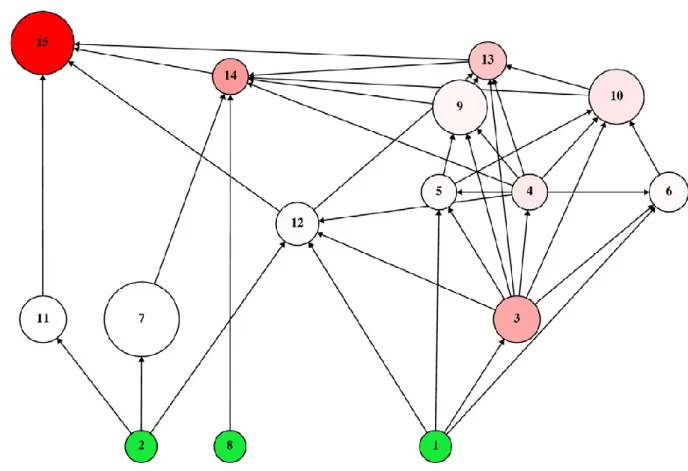
We analyse a single food web, containing three producers (species #1, #2 and #8), one top 103
predator (species #15) and 11 intermediate species (Figure 1). The network is of intermediate 104
size (N = 15 living trophic groups), so it is still manageable for dynamical simulations (using 105
several population dynamical parameters) but already interesting enough for topological 106
studies (focusing only on food web structure). The topology of the network is arbitrary but a 107
similar study of 100 randomly generated, comparable networks is already in progress.
108 109
5 Methods
110 111
Network structure 112
113
In order to quantify the structural importance of network nodes, first, we consider the food 114
web as an undirected network where effects can spread in any direction (from prey to predator 115
and from predator to prey). These are clearly not only energy flows but trophic interactions in 116
a broader sense. A range of network indices can be used for quantifying the positional 117
importance of nodes in undirected networks (note that some of these indices have versions 118
adapted to directed networks too). Since we still do not understand the structure to dynamics 119
relationship, it makes sense to test several structural indices and clarifying their relationship 120
with dynamics. The structural indices are clearly not independent of each other but we study 121
relationships between structural versus simulated metrics and investigate which structural 122
indices are correlating best with simulated non-additive effects.
123 124
Degree and weighted degree (D, wD) 125
126
The most local network centrality index is the degree of a node (D). This is the number of 127
other nodes connected directly to it. In a food web, the degree of a node i (Di) is the sum of its 128
preys and predators. In the case of weighted networks, the weighted degree of node i (wDi) 129
equals the sum of weights on links adjacent to node i (Wassermann and Faust 1994). Degree 130
and weighted degree can be calculated by the UCINET programme (Borgatti et al. 2002).
131 132
Betweenness centrality (BC) 133
134
This measure of positional importance quantifies how frequently a node i is on the shortest 135
path between every pair of nodes j and k. This index is called ”betweenness centrality” (BC), 136
used routinely in social network analysis (Wassermann and Faust 1994) and we calculated it 137
using the UCINET programme (Borgatti et al. 2002). The standardised index for node i (BCi) 138
139 is:
140
𝐵𝐶𝑖 = 2 ∑
𝑔𝑗𝑘(𝑖) 𝑗<𝑘 𝑔𝑗𝑘
(𝑁−1)(𝑁−2) (1)
141
142
6
where i ≠ j and k. gjk is the number of equally shortest paths between nodes j and k, and gjk (i) 143
is the number of these shortest paths to which node i is incident (of course, gjk may equal 144
one). The denominator is twice the number of pairs of nodes without node i. This index thus 145
measures how central a node is, in the sense of being incident to many shortest paths in the 146
network. If BCi is large for trophic group i, it means that deleting this group will more affect 147
many rapidly spreading effects in the web.
148 149
Closeness centrality (CC) 150
151
Closeness centrality (CC) is a measure quantifying how short are the minimal paths from a 152
given node to all others (Wassermann and Faust 1994) and is again calculated using UCINET 153
(Borgatti et al. 2002). The standardised index for a node i (CCi) is:
154 155
𝐶𝐶𝑖 = ∑𝑁−1𝑑
𝑁 𝑖𝑗
𝑗=1 (2)
156
157
where i≠j and dij is the length of the shortest path between nodes i and j in the network. This 158
index thus measures how close a node is to others. The larger CCi is for trophic group i, the 159
more directly deleting this group will affect the majority of other groups.
160 161
Positional importance based on indirect chain effects (TIn and WIn) 162
163
We can assume a network with undirected links where trophic effects can spread in many 164
directions without bias. Indirect effects do spread in both bottom-up and top-down directions 165
through trophic links and, as a result, horizontally, too. We first consider an unweighted 166
network. Here, we define an,ij as the effect of j on i when i can be reached from j in n steps.
167
The simplest mode of calculating an,ij is when n=1 (i.e. the effect of j on i in 1 step): a1,ij = 168
1/Di, where Di is the degree of node i (i.e. the number of its direct neighbours including both 169
prey and predator species). We assume that indirect chain effects are multiplicative and 170
additive. For instance, we wish to determine the effect of j on i in 2 steps, and there are two 171
such 2-step pathways from j to i: one is through k and the other is through h. The effects of j 172
on i through k is defined as the product of two direct effects (i.e. a1,kj×a1,ik), this is why 173
multiplicative. Similarly, the effect of j on i through h equals to a1,hj,1×a1,ih. To determine the 174
7
2-step effect of j on i (a2,ij), we simply sum up those two individual 2-step effects (i.e. a2,ij= 175
a1,kj×a1,ik+ a1,hj×a1,ih) in an additive way (Jordán et al. 2003).
176
When the effect of step n is considered, we define the effect received by species i from 177
all species in the same network as:
178 179
𝜑𝑛,𝑖 = ∑𝑁𝑗=1𝑎𝑛,𝑗𝑖 (3) 180
181
which is equal to 1 (i.e. each species is affected by the same unit effect.). Furthermore, we 182
define the n-step effect originated from a species i as:
183 184
𝜎𝑛,𝑖 = ∑𝑁𝑗=1𝑎𝑛,𝑗𝑖 (4) 185
186
which may vary among different species (i.e. effects originated from different species may be 187
different). Here, we define the topological importance of species i when effects “up to” n step 188
are considered as:
189 190
𝑇𝐼𝑖𝑛 =∑𝑛𝑚=1𝑛𝜎𝑚,𝑖 =∑𝑛𝑚=1∑𝑛𝑁𝑗=1𝑎𝑚,𝑗𝑖 (5) 191
192
which is simply the sum of effects originated from species i up to n steps (one plus two plus 193
three…up to n) averaged over by the maximum number of steps considered (i.e. n ). For the 194
undirected network with weighted links, all effects are defined in the same way as above with 195
the exception of 1-step effects, which is defined as:
196 197
𝑎1,𝑖𝑗= 𝜀𝜇𝑖𝑗
𝑖 (6)
198
199
where μi is the sum of the strength of the links connected to i and εij is the strength of the link 200
connecting i and j. The weighted approach of calculating 2-step effects (i.e. a2,ij) was 201
originally developed by Godfray and colleagues for assessing apparent competition in host- 202
parasitoid communities (Müller and Godfray 1999; Müller et al. 1999; Rott and Godfray 203
2000). Furthermore, we define WIin as the topological importance of species i for networks 204
with weighted links when effects “up to” n steps are considered:
205 206
8
𝑊𝐼𝑖𝑛 = ∑𝑛𝑚=1𝑛𝜎𝑚,𝑖= ∑𝑛𝑚=1∑𝑛𝑁𝑗=1𝑎𝑚,𝑗𝑖 (7) 207
208
We analysed indirect effects of different maximum length (n = 1, 3, 10); these indices can be 209
calculated by the Cosbi Graph software (Valentini and Jordán 2010).
210 211
Status index and its components (s, s`, Δs) 212
213
We also consider the food web as a directed acyclic graph (DAG). In this case, we can apply 214
different network indices for measuring the positional importance of nodes. The status of 215
node i (si) in a hierarchy is the sum of its dij distance values to all other j nodes in the network.
216
The contrastatus of this i node (s`i) is the same calculated after reversing the sign of all links 217
in the graph. The net status of this node i (Δsi) equals the difference of the two former indices:
218 219
𝛥𝑠𝑖 = 𝑠𝑖− 𝑠 𝑖 (8) 220
221
These indices have been introduced in sociometry (Harary 1959) and applied subsequently to 222
ecological problems (Harary 1961). We may note that this latter attempt to quantify the 223
relative importance of species in ecological communities, based on their network position was 224
a pioneering effort not followed by biologists for decades (see Mills et al. 1993; but even the 225
qualitative discussion of species importance came only years later Paine 1966). These indices 226
can be calculated by the Cosbi Graph software (Valentini and Jordán 2010).
227 228
Keystone index and its components (K, Kbu, Ktd, Kdir, Kindir).
229 230
The keystone index (K, Jordán et al. 1999) is derived from earlier works on DAGs (Harary 231
1959; 1961). The keystone index of a species i (Ki) is defined as:
232 233
𝐾𝑖 = 𝐾𝑏𝑢,𝑖+ 𝐾𝑡𝑑,𝑖 = 𝐾𝑑𝑖𝑟,𝑖+ 𝐾𝑖𝑛𝑑𝑖𝑟,𝑖 = ∑ 𝑑1
𝑐
𝑛𝑐=1 (1 + 𝐾𝑏𝑐) + ∑ 𝑓1
𝑒
𝑚𝑒=1 (1 + 𝐾𝑡𝑒) (9) 234
235
where n is the number of predators eating species i, dc is the number of prey species of its cth 236
predator and Kbc is the bottom-up keystone index of the cth predator. And symmetrically, m is 237
the number of prey eaten by species i, fe is the number of predators of its eth prey and Kte is the 238
top-down keystone index of the eth prey. For node i, the first sum in the equation (i.e.
239
9
∑1/dc(1+Kbc)) quantifies the bottom-up effect (Kbu,i) while the second sum (i.e. ∑1/fe(1+Kte)) 240
quantifies the top-down effect (Ktd,i). After rearranging the equation, terms including Kbc and 241
Kte (i.e. ∑Kbc/dc + ∑Kte/fe) refer to indirect effects for node i (Kindir,i), while terms not 242
containing Kbc and Kte (i.e. ∑1/dc + ∑1/fe) refer to direct ones (Kdir,i). Both Kbu,i + Ktd,i and 243
Kindir,i + Kdir,i equals Ki. The degree of a node in a network (D) characterises only the number 244
of its connected (neighbour) points, while the keystone index gives information also on how 245
these neighbours are connected to their neighbours. It quantifies only vertical interactions 246
(like trophic cascades), without considering horizontal ones (like apparent competition), 247
separating indirect from direct, as well as bottom-up from top-down effects in food webs.
248
These indices can also be calculated by the Cosbi Graph software (Valentini and Jordán 249
2010).
250
We used 18 positional importance indices to quantify the relative importance of nodes 251
in the food web (D, wD, BC, CC, TI1, TI3, TI10, WI1, WI3, WI10, s, s`, Δs, K, Kbu, Ktd, Kdir, 252
Kindir). Although all of these indices say something about the positional importance, also all of 253
them are different. Some of them (e.g. D) are local, not considering indirect effects (i.e. the 254
neighbours of neighbours) while others are non-local or mesoscale indices (e.g. BC, TI10).
255
Some of them consider binary interactions (e.g. TI3), while others can quantify weighted 256
networks (e.g. WI3). Finally, some of them characterize undirected (e.g. D), while others do 257
directed networks (e.g. s, K).
258
Clearly, there are several more indices, still quantifying node centrality in networks 259
(e.g. information centrality, IC). Here we focus on some of the most used and probably more 260
promising indices (McDonald-Madden et al. 2016). Apart from their nature, these particular 261
indices differ also from the viewpoint of robustness, for example. Some of them are more, 262
while others are less sensitive to incomplete data (sampling, see Fedor and Vasas 2009).
263
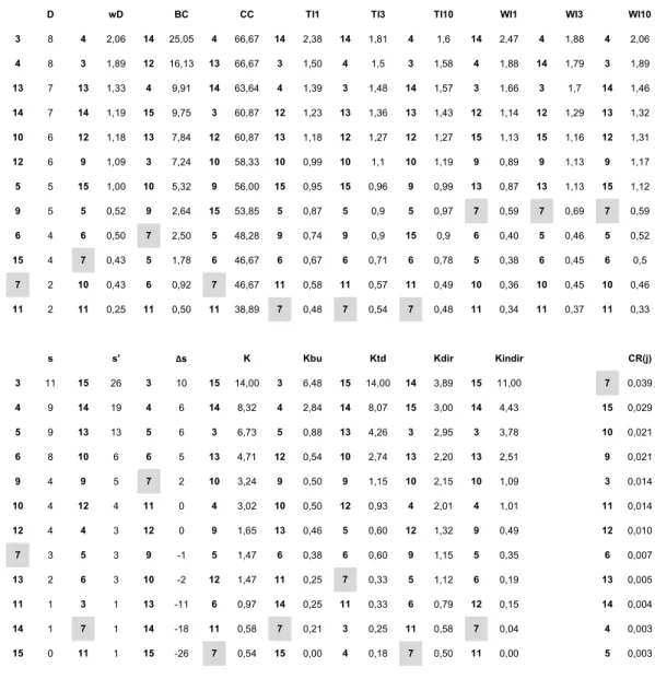
Table 1 shows the values of all these indices for the nodes of the food web (for the results of 264
statistical analyses, see Table 2 below).
265 266
Network dynamics 267
268
For modelling the dynamic behaviour of these trophic networks, we extended an earlier model 269
of ours, focusing on overfishing in small model food webs (Mόréh et al. 2009). The dynamics 270
of each species can be described by the following differential equation:
271 272
10
𝑑𝑁𝑖
𝑑𝑡 = 𝑟𝑖𝑁𝑖(1 −𝑁𝐾𝑖
𝑖) + ∑𝜌=𝑟𝑒𝑠𝑜𝑢𝑟𝑐𝑒𝑠𝑁𝑖𝜀𝑖𝜌𝑁𝑁𝜌ℎ𝜔𝑖𝜌
0ℎ+𝜔𝑖𝜌𝑄𝑖𝜌− ∑𝑐=𝑐𝑜𝑛𝑠𝑢𝑚𝑒𝑟𝑠𝑁𝑐𝜀𝑐𝑖 𝑁𝑖ℎ𝜔𝑐𝑖
𝑁0ℎ+𝜔𝑐𝑖𝑄𝑐𝑖− 𝑑𝑖𝑁𝑖 273
(10) 274
275
where Ni means the abundance of species i; ri and Ki are the rate of increase and carrying 276
capacity of the logistic model, respectively. These quantities characterise the basal species 277
only (i=1,2,8, see Figure 1); di is the mortality rate of consumer species i. Holling type-III 278
(h=2) functional response refers to the realized fraction of i’s maximum ingestion rate when 279
consuming its prey species. ωiρ is species i’s relative consumption rate when consuming ρ, N0
280
is the half-saturation density and Qiρ is the sum of the abundances of the resources i can 281
consume. The relative consumption rates are inversely proportional to the number of 282
resources: ωi = 1/n.
283
In order to focus on how network topology influences dynamics, we did not model the 284
consumption or conversion rates of species explicitly and assumed that the strength of a 285
predator-prey link (ε) is solely proportional to the number of preys (εi = 1/n). Similarly, 286
almost every parameter was fixed (Ki = 1, ri = 1 for basal species, εi = ωi = 1/n) except 287
mortality rates (di), which were chosen from a biologically plausible range to achieve a stable 288
coexistence of all 15 species. We searched for different sets of di-combinations that lead to 289
robust coexistence.
290
For the integration of the set of ODEs described in the previous equation, we used the 291
CVODE code with adaptive backward differentiation scheme (Hindmarsh et al. 2005). For all 292
simulations, all initial abundances were set to 1 and the system was integrated over T = 293
20.000 time steps (since one step is a unit change of population size of the fastest-growing 294
organisms, say phytoplankton, this range roughly corresponds to a decadal time-scale, like 20- 295
30 years). If the abundance of any species decreased below the threshold of 10-6, we 296
considered it to be extinct and the integration was terminated. If the dynamics is settled to a 297
fixed point during the integration and the solution was locally asymptotically stable, the 298
systems were used for sensitivity analysis, see below. We note that we have found limit cycles 299
in less than 1% of the simulations and we have not found chaotic solutions. The limit cycles 300
were excluded from further investigations.
301 302
Sensitivity analysis 303
304
11
Having selected the robust webs in this manner, sensitivity analysis became possible. We 305
perturbed only the 12 consumer species, so the producer species #1, #2 and #8 were part of 306
the dynamical system but their community effects were not evaluated. We applied the 307
following method in all cases. We selected a set of di parameters where the web was robustly 308
present, and run the integration again. After the dynamical equilibrium was settled, we 309
perturbed the mortality rate of the species in question by increasing it by 10%. Our in silico 310
sensitivity analysis can be considered as press perturbation experiments (sensu Bender et al.
311
1984) and we trace also indirect, not only the direct consequences.
312
Following single-species perturbations, we perturbed species in all possible pairwise 313
combinations as well. In the case of pairwise perturbations, the perturbations on species i and 314
species j were parallel in time and they were of equal strength (10% increase of di and dj).
315 316
Community response 317
318
We were interested in the effect of perturbing species i on all other species j in the system and 319
we determined the community response to this perturbation (CRi) as the sum of all these 320
answers (without considering the feedback of perturbing species i on itself, i.e. self-effects).
321
So, if Ni(*)t is the population size of species i at time t in the reference simulation and 322
Ni(j)t is the population size of species i at time t in a simulation where species j was disturbed, 323
then the individual answer of a species i to perturbing species j is 324
325
𝑅𝑗 =𝑁𝑁𝑖(𝑗)𝑡
𝑖𝑡 (11)
326
327
and this can be larger or smaller than 1 (the former meaning increased population size as a 328
response to perturbation and the latter meaning decreased population size as a response to 329
perturbation). The community response to the single-species perturbation on species j is 330
331
𝐶𝑅𝑗 = ∑ |𝑁𝑁𝑖(𝑗)𝑡
𝑖𝑡 − 1|
𝑛𝑖=1 ⁄14,(𝑖 ≠ 𝑗) (12) 332
333
In case of pairwise perturbations, the community response to perturbing species j and k in 334
parallel is 335
336
12 𝐶𝑅[𝑗𝑘]= ∑ |𝑁𝑖(𝑗,𝑘)𝑡𝑁
𝑖𝑡 − 1| /
𝑛𝑖=1 13, (𝑖 ≠ 𝑗 ≠ 𝑘) (13) 337
338 339
A question that is of both technical and philosophical nature is whether we prefer small 340
effects (even if negative) or positive effects (even if large). In other words, we want to 341
minimize our impact on nature (small negative better than large positive) or to help it (large 342
positive better than small negative). Because we preferred the former scenario (small effect), 343
we calculated the absolute values of the differences from 1 (meaning no change). A number 344
of alternative response functions are used in community ecology (Livi et al. 2011; Hurlbert 345
1997; Okey 2004): our function is most similar to the interaction strength index (ISI).
346
Comparing the effects of single-species and pairwise perturbations by 347
348
𝑁𝐴[𝑗𝑘]= |𝐶𝑅𝑗+ 𝐶𝑅𝑘− 𝐶𝑅[𝑗𝑘]| (14) 349
350
quantifies the non-additivity of the effects of perturbing species j and k in parallel. Smaller NA 351
values mean large additivity. Non-additive effects can be realized in two ways. First, the small 352
effects of the single-species [j] and [k] perturbations can be escalated in a [j k] pairwise 353
perturbation. Second, the large effects of the single-species [j] and [k] perturbations can be 354
dampened in a [j k] pairwise perturbation.
355 356
Classification of node pairs 357
358
Since the food web contains 15 nodes but we do not perturb the 3 producer species, we have 359
12 single-species perturbations and (12+11)/2 = 66 combinations for pairwise perturbations.
360
These 66 combinations of two species can be characterized by several ways.
361 362
Centrality 363
364
We are interested in the pairwise perturbation of species combinations where each species 365
belongs to the most central 5 nodes of the network, according to each of the 18 topological 366
indices we used. The pairwise combinations of the 5 highest-centrality nodes provide 10 367
(unordered) species pairs. For an example, we have species #14, #4, #3, #13 and #12 on the 368
top of the centrality rank based on TI3, so we study if their pairwise combinations ([14 4], [14 369
13
3], [14 13], [14 12], [4 3], [4 13], [4 12], [3 13], [3 12] and [13 12]) have different community 370
responses than other species pairs. Note that we have 15 species pairs for D, since there is a 371
tie between species #10 and #12 in the D-rank (Table 1) and we decided to consider both as 372
highest-centrality nodes in the network; 6 species provide 15 pairwise combinations. All of 373
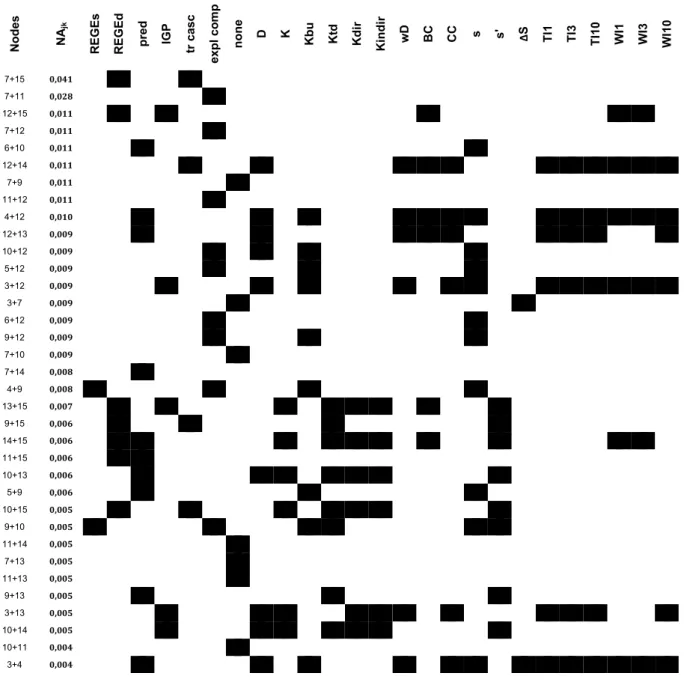
these categorizations, according to the 18 structural indices are seen in Table 3.
374 375
Regular equivalence 376
377
We used the regular equivalence measure (REGE, see Lorrain and White 1971; Everett and 378
Borgatti 1991; Luczkovich et al. 2003) for defining network roles in the food web. This 379
measure quantifies the similarity between the positions of network nodes i and j, based on 380
their network position (this approach is a general version of the quite similar, classical 381
concept of trophospecies, Yodzis and Winemiller 1999). Their composition is based on the 382
REGE analysis. The dendrogram that expresses the similarity can be cut at any threshold level 383
in order to define and create aggregated functional groups. We were interested in pairs of 384
species of similar (REGEs) and dissimilar (REGEd) network position. In Figure 2, we show 385
the dendrogram and we mark a group of similarly-positioned species (REGEs) in blue, while 386
the most distant branch of the dendrogram (species #15) as well as its highest-level branching 387
point in red (this group provides the REGEd category when combined with any of the others).
388
Producers (marked in green) are not considered in the analysis, otherwise, they would provide 389
the highest branching point in the dendrogram. Both of these categorizations are seen in Table 390
3: node pairs in very similar (REGEs; [9 10], [4 9], [4 10] and [5 6]) and very different 391
(REGEd; all of the 11 [15 i] pairs) network positions.
392 393
Modules 394
395
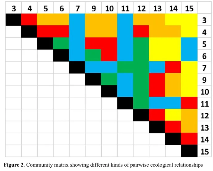
Based on the ecological characteristics of interspecific interactions, we categorize all species 396
pairs in the food web as (1) being in predator-prey interaction, (2) being in intra-guild 397
predation (IGP) interaction, (3) being in a trophic cascade interaction, (4) being exploitative 398
competitors or (5) none of the above (including apparent competition). The colouring of the 399
community matrix on Figure 3 shows this classification and group identities are shown in 400
Table 3: we have 14 pairs in prey-predator relationship („pred”), 13 intra-giuld predations 401
(„IGP”), 11 trophic cascades („tr casc”), 11 exploitative competitions („expl comp”) and 17 402
relationships belonging to none of the above („none”).
403
14 404
Statistical analysis 405
406
In the case of single-species perturbations, we had numerical values (Table 1) and the 407
relationship between structural importance and community response was evaluated by the 408
Spearman correlation (rho and p-values given in Table 2). In the case of pairwise 409
perturbations, we had categorical values (Table 3) and the relationship between structural 410
importance and community response was evaluated by Mann-Whitney test (Table 4).
411 412
Results 413
414
Table 1 shows the topological characteristics of the 12 graph nodes that are of interest for the 415
perturbation experiments (values for species #1, #2 and #8 are not shown). Based on local 416
measures, species #3 and #4 are the most central ones in the binary (D = 8), while species #4 417
is the single most central one in the weighted (wD = 2,06) network. Classical non-local 418
centrality measures suggest the key position of either species #14 (BC = 25,05) or species #4 419
and #13 (CC = 66,67). Topological importance identifies species #14 for shorter (TI1 = 2,38, 420
TI3 = 1,81) and species #4 for longer (TI10 = 1,6) pathways. Based on weighted importance, 421
the same species dominate but species #4 gets dominance earlier as pathway length increases 422
(WI3 = 1,88, WI10 = 2,06), preceding species #14 that is still the most central one for the most 423
local interactions (WI1 = 2,47).
424
Hierarchical indices suggest different key nodes for the directed version of the food 425
web. Species #3 has the highest status (s = 11) and species #15 has the highest contra-status 426
(s` = 26), and the net status index identifies these two species with the most extreme values 427
(∆s). Based on net status, species #11 and #12 are the most balanced ones (∆s = 0). The 428
keystone index suggests species #3 based on bottom-up (Kbu = 6,48) and species #15 based on 429
top-down (Ktd = 14) effects, while species #14 based on direct (Kdir = 3,89) and species #15 430
based on indirect (Kindir = 11) effects. The overall key species is suggested to be species #15 431
(K = 14).
432
Based on these 18 topological indices of positional importance, we can identify 5 433
species that are of critical importance in this trophic network (species #3, #4, #13, #14 and 434
#15). Note that species #3 is more important in unweighted (binary) networks, species #4 is 435
more important in undirected (symmetrical) ones, species #15 is in key position only in the 436
directed network and species #13 is important based only on CC (undirected, unweighted).
437
15
But species #14 has highest centrality based on both directed (Kdir) and undirected (BC) as 438
well as both binary (TI1) and weighted (WI1) measures. All in all, species #14 can be clearly 439
suggested to be the most critical node in this network.
440
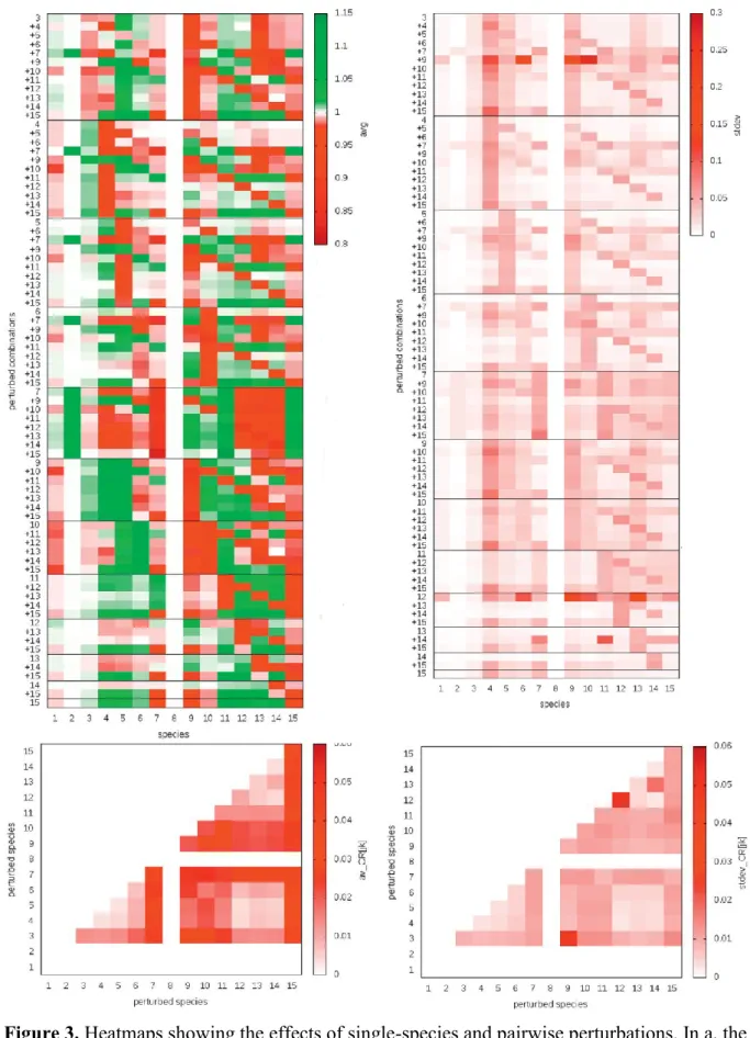
Figure 4 shows the species-specific answers of single-species and pairwise 441
perturbations (the average for several simulations shown in Figure 4a). Some perturbations 442
have predominantly positive effects on others (like [9 15], the pairwise perturbation of species 443
#9 and #15), this is indicated by a larger number of green cells in the corresponding row of 444
Figure 4a. Some species are typically positively influenced by perturbations (like species 445
#11), this is indicated by the larger number of green cells in the corresponding column of 446
Figure 4a. Symmetrically, mostly negative effects are caused by perturbing [4 5] and the 447
impacts are mostly negative on species #7. This detailed information is useful for better 448
understanding the mechanistic details of community dynamics but the community response 449
function we used does not consider the sign, only the strength of responses (otherwise strong 450
positive and strong negative effects extinct each other and show weak community answer).
451
The summarized community responses are shown in Figure 4c and the statistical analysis 452
concerns these community responses, not the species-specific responses on Figure 4a.
453
The consistency of the previous results can be calculated by the standard deviation of 454
individual responses during the simulations. Figures 4b and 4d show this information for the 455
species-specific and for the community responses, respectively. Some perturbations have 456
quite consistent effects on others (like [5 14]), with predictable results (mostly white cells in 457
the corresponding row of Figure 4b), and some species are quite consistently impacted (like 458
species #3, see the white cells in the corresponding column of Figure 4b). Similarly, some 459
perturbations give quite inconsistent results (like [3 9]) and some species are quite 460
inconsistently impacted (like species #4).
461
The numerical values of community responses generated by single-species 462
perturbations are presented in Table 1 (CRj). Here we see only 12 values since producers 463
(species #1, #2 and #8) have not been perturbed. For visualization, see Figure 1. It can be seen 464
that perturbing species #7 generates the largest community answer (note that D7 = 2, so this 465
species cannot be considered a hub species, and it does not belong to the highest-centrality 466
nodes according to any index).
467
Correlation coefficients between community importance quantified by the various 468
topological indices and community importance quantified by the effects of single-species 469
perturbations are given in Table 2. Interestingly, no structural index shows significant 470
16
correlation with dynamical importance. The highest (still non-significant) and lowest p-values 471
characterize the Kindir and the D indices, respectively.
472
Pairwise species combinations are ranked according to the non-additivity of their 473
effects (Table 3). The existence of non-additive effects is not surprising (e.g. Kareiva 1994;
474
Wootton 1994) but their network-based, quantitative understanding is incomplete. The top of 475
the ranking shows the least additive effects of perturbing a [j k] pair versus perturbing them 476
separately ([j] + [k]). Combinations [7 15] and [7 11] give the least additive results, while 477
combinations [6 7] and [3 10] give the most additive answers. The single-species perturbation 478
of species #7 gives the largest community response (see Table 1) and this species is a member 479
of most of the pairwise combinations generating the least additive effects. Without species #7, 480
[12 15] gives the least additive effect and [6 7] gives the most additive effect with species #7.
481
The summed community responses to perturbing species [j] and [k] do not necessarily 482
predict the community response to [j k] perturbations. In Figure 5, we can see how pairwise 483
effects and single effects are related to each other for particular pairs of species. On the y axis, 484
we see the pairwise community response values (CRjk), while on the x axis we see the sum of 485
the single-species community response values (CRj + CRk). Points on the x = y line show 486
combinations where it does not matter whether the two species are perturbed separately or in 487
combinations (high additivity). Below the line, we have non-additive, dumping effects (e.g. [7 488
15], [7 11]) and above the line we have non-additive, escalating effects (only [3 9]). We can 489
say that additivity is generally quite high.
490
If we look at the rank positions of the 25 different categories of species combinations, 491
we find that 2 of them differ significantly from the rest (Table 4). Non-additivity of pairwise 492
perturbations is higher if the species pair has high ∆s-values or if they are (exploitative) 493
competitors. Finally, we note that higher non-additivity values are generally accompanied 494
with a larger variability of the pairwise community response values (Figure 6). This means 495
that if the perturbation of species i and j produces more additive effects, the community 496
response to their pairwise perturbation will be also more predictable (Spearman’s rho = - 497
0,094).
498 499
Conclusions and future directions 500
501
We have found significant effects of network topology on the additivity of pairwise 502
perturbations. However, for single-species perturbations, we have found no significant 503
relationships between food web position and community response.
504
17
We determined the trophic components of highest positional importance, the 505
dynamical effects of single-species and pairwise perturbations and the additivity of pairwise 506
species perturbations in a food web simulation model. We emphasize that the response 507
function we have chosen does not provide information about positive and negative effects 508
(increase or decrease of population size), only about large and small effects (the change in 509
population size). This is supported by a conservation philosophy suggesting that minimizing 510
the human impact (size of change) might be preferred over trying to help natural systems 511
(direction of change).
512
We found that, according to the dynamical model we used, food web structure is a 513
poor predictor of dynamics. The effects of single-species perturbations show no correlation 514
with the position of the species in the food web. Yet, we can find that weighted measures 515
perform better than unweighted ones (WIn better than TIn and wD better than D). Also, 516
indirect measures almost always perform better than direct ones (TIn and WIn better than wD 517
and D, the exception is TI10). These support earlier findings of the poor predictive power of a 518
local and binary view on networks (Jordán et al. 2008; Livi et al. 2011). Based on our results, 519
we can state that pairwise species perturbations have non-additive and almost always 520
dampening effects if the two perturbed species are competitors or if they have high net status 521
values (Δs).
522
Better understanding the topological effects on additivity can be useful for systems- 523
based conservation (e.g. multi-species fisheries management). Clearly, the sustainability of 524
fisheries is a much more complicated issue: predicting interaction strength between trophic 525
groups (or species) is not easy even in small systems of just a few species but there are recent 526
developments for multi-species systems (based on a large number of attributes, including 527
simplistic food web properties like degree, Berlow et al. 2009). Apart from better 528
understanding the topological basis of sustainable ecosystems, it is clear that several other 529
factors need to be addressed for sustainability research: these include economic aspects (like 530
profitability, see Norrström et al. 2017) and fisheries management issues (like focusing on 531
stock size versus fishing pressure, see Farcas and Rossberg 2016). Clarifying topological 532
constraints can only be possible without considering all other aspects but these mathematical 533
constraints must then be integrated with additional knowledge. Assessing MSY in a multi- 534
species context may use information provided by this kind of analysis: the maximum yield 535
values determined for a particular pair of species might be changed as a function of their 536
topological relationship. This makes MSY assessment more complicated but also more 537
18
system-based and holistic. Our purpose was to demonstrate how network analysis can be used 538
for quantifying these constraints.
539
One of the key future extensions of this study is to investigate the generality of the 540
results (same analysis is under investigation for 100 networks). General results on favourable 541
topologies for dampening pairwise perturbations could really serve the basis of system-based 542
conservation. Given that some general rules will emerge, these can be applied to real 543
databases: in the case of fisheries on species x, we should be able to determine which other 544
species y could also be fished, in combination with x, such that the combined impact is non- 545
additive and favourable for the system (minimizing the impact). Topological analyses do not 546
solve ecological problems themselves but they can help better understanding some basic 547
constraints on ecosystem dynamics. Several additional factors can then be added and 548
combined with it.
549
Here we addressed only the community-wide effects of heavy perturbations (e.g.
550
fishing) on a single species or their pairwise combinations. But we think this is quite an 551
important component of MSY, especially since our model provides a multi-species context for 552
the problem. Understanding the relationship between single-species and multi-species 553
perturbations (fisheries) is a major step towards better understanding additivity. If pairwise 554
perturbations are more additive, the predictive value of single-species MSY-assessments is 555
clearly higher (Walters et al. 2005). We have presented topological constraints on additivity:
556
based on the network position of two species we can try to predict whether their pairwise 557
perturbation will result in summed or dampened effects.
558 559
Acknowledgements 560
FJ was supported by the National Research, Development and Innovation Office – NKFIH, 561
grant number K 116071. Juliana Szabό is kindly acknowledged for excellent comments on the 562
manuscript.
563 564
References 565
566
Allesina, S. and Bodini, A. 2004. Who dominates whom in the ecosystem? Energy flow 567
bottlenecks and cascading extinctions. J. Theor. Biol. 230: 351-358.
568
Allesina, S., Bodini, A. and Bondavalli, C. 2006. Secondary extinctions in ecological 569
networks: bottlenecks unveiled. Ecol. Model. 194: 150-161.
570
19
Beddington, J. R. and May, R. M. 1980. Maximum sustainable yields in systems subject to 571
harvesting at more than one trophic level. Math. Biosci. 51: 261-281.
572
Bender, E. A. et al. 1984. Perturbation experiments in community ecology: theory and 573
practice. Ecology 65: 1-13.
574
Berlow, E. L. et al. 2009. Simple prediction of interaction strengths in complex food webs.
575
Proc Natl Acad Sci USA 106: 187–191.
576
Borgatti, S. P. et al. 2002. Ucinet for Windows: Software for Social Network Analysis.
577
Harvard: Analytic Technologies.
578
Chakraborty, S. K. et al. 1997. Estimates of growth, mortality, recruitment pattern and 579
maximum sustainable yield of important fishery resources of Maharashtra coast. Ind. J. Mar.
580
Sci. 26: 53-56.
581
Eklöf, A. and Ebenman, B. 2006. Species loss and secondary extinctions in simple and 582
complex model communities. J. Anim. Ecol. 75: 239-246.
583
Estrada, E. 2007. Characterisation of topological keystone species: local, global and “meso- 584
scale” centralities in food webs. Ecol. Compl. 4: 48-57.
585
Everett, M. G. and Borgatti, S. 1991. Role colouring a graph. Math. Soc. Sci. 21: 183-188.
586
Farcas, A. and Rossberg, A. G. 2016. Maximum sustainable yield from interacting fish stocks 587
in an uncertain world: two policy choices and underlying trade-offs. ICES J. Mar. Sci. 73:
588
2499–2508.
589
Fedor, A. and Vasas, V. 2009. The robustness of keystone indices in food webs. J. Theor.
590
Biol. 260: 372–378.
591
Geček, S. and Legović, T. 2012. Impact of maximum sustainable yield policy on competitive 592
community. J. Theor. Biol. 307: 96-103.
593
Guillen, J. et al. 2013. Estimating MSY and MEY in multi-species and multi-fleet fisheries, 594
consequences and limits: an application to the Bay of Biscay mixed fishery. Marine Policy 40:
595
64–74.
596
Hannesson, R. 1983. Optimal harvesting of ecologically interdependent fish species. J. Env.
597
Econ. Manag. 10: 329-345.
598
Harary, F. 1959. Status and contrastatus. Sociometry 22: 23-43.
599
Harary, F. 1961. Who eats whom? General Systems 6: 41-44.
600
Hindmarsh, A. C. et al. 2005. SUNDIALS: Suite of Nonlinear and Differential/Algebraic 601
Equation Solvers. ACM Trans. Math. Softw. 31: 363-396.
602
Hollowed, A. B. et al. 2000. Are multispecies models an improvement on single-species 603
models for measuring fishing impacts on marine ecosystems? ICES J. Mar. Sci. 57: 707–719.
604
20
Hurlbert, S. H. 1997. Functional importance vs keystoneness: reformulating some questions in 605
theoretical biocenology. Austr. J. Ecol. 22: 369-382.
606
Jordán, F. 2009. Keystone species in food webs. Phil. Trans. Roy. Soc., London, series B 364:
607
1733-1741.
608
Jordán, F. et al. 2003. Quantifying the importance of species and their interactions in a host- 609
parasitoid community. Comm. Ecol. 4: 79-88.
610
Jordán, F. et al. 2008. Identifying important species: a comparison of structural and functional 611
indices. Ecol. Model. 216: 75-80.
612
Jordán, F. et al. 2002. Species positions and extinction dynamics in simple food webs. J.
613
Theor. Biol. 215: 441-448.
614
Jordán, F. et al. 1999. A reliability theoretical quest for keystones. Oikos 86: 453-462.
615
Kareiva, P. 1994. Higher order interactions as a foil to reductionist ecology. Ecology 616
75: 1527-1528.
617
Legović, T. and Geček, S. 2010. Impact of maximum sustainable yield on independent 618
populations. Ecol. Model. 221: 2108–2111.
619
Legović, T. et al. 2010. Maximum sustainable yield and species extinction in ecosystems.
620
Ecol. Model. 221: 1569–1574.
621
Legović, T. and Geček, S. 2012. Impact of maximum sustainable yield on mutualistic 622
communities. Ecol. Model. 230: 63-72.
623
Livi, C. M. et al. 2011. Identifying key species in ecosystems with stochastic sensitivity 624
analysis. Ecol. Model. 222: 2542-2551.
625
Lorrain, F. and White, H. C. 1971. Structural equivalence of individuals in social networks. J.
626
Math. Soc. 1: 49-80.
627
Luczkovich, J. J. et al. 2003. Defining and measuring trophic role similarity in food webs 628
using regular equivalence. J. Theor. Biol. 220: 303–321.
629
Maunder, M. N. 2002. The relationship between fishing methods, fisheries management and 630
the estimation of maximum sustainable yield. Fish and Fisheries 3: 251–260.
631
May, R. M. et al. 1979. Management of multispecies fisheries. Science 205: 267-277.
632
McDonald-Madden, E. et al. 2016. Using food-web theory to conserve ecosystems. Nat.
633
Comm. 7: 10245.
634
Mills, L. S. et al. 1993. The keystone-species concept in ecology and conservation.
635
BioScience 43: 219-224.
636
Móréh, Á. et al. 2009. Overfishing and regime shifts in minimal food web models. Comm.
637
Ecol. 10: 236-243.
638
21
Mueter, F. J. and Megrey, B. A. 1980. Using multi-species surplus production models to 639
estimate ecosystem-level maximum sustainable yields. Fish. Res. 81: 189–201.
640
Müller, C. B. et al. 1999. The structure of an aphid–parasitoid community. J. Anim. Ecol. 68:
641
346–370.
642
Müller, C. B. and Godfray, H. C. J. 1999. Indirect interactions in aphid-parasitoid 643
communities. Res. Pop. Ecol. 41: 93-106.
644
Norrström, N. et al. 2017. Nash equilibrium can resolve conflicting maximum sustainable 645
yields in multi-species fisheries management. ICES J. Mar. Sci. 74: 78–90.
646
Okey, T. A. 2004. Shifted community states in four marine ecosystems: some potential 647
mechanisms. PhD thesis, University of British Columbia, Vancouver.
648
Paine, R. T. 1966. Food web complexity and species diversity. Am. Nat. 100: 65-75.
649
Pauly, D. 1979. Theory and management of tropical multispecies stocks: A review, with 650
emphasis on the Southeast Asian demersal fisherics. ICLARM Studies and Reviews No. 1, 35 651
p., Manila.
652
Pimm, S. L. 1980. Food web design and the effect of species deletion. Oikos 35: 139-149.
653
Pocock, M. J. O. et al. 2011. Succinctly assessing the topological importance of species in 654
flower–pollinator networks. Ecol. Compl. 8: 265–272.
655
Quince, C., Higgs, P. G. and McKane, A. J. 2005. Deleting species from model food webs.
656
Oikos 110: 283-296.
657
Rott, A. S. and Godfray, H. C. J. 2000. The structure of a leafminer-parasitoid community. J.
658
Anim. Ecol. 69: 274-289.
659
Schaefer, M. B. 1991. Some aspects of the dynamics of populations important to the 660
management of the commercial marine fisheries. Bull. Math. Biol. 53: 253-279.
661
Valentini, R. and Jordán, F. 2010. CoSBiLab Graph: the network analysis module of 662
CoSBiLab. Env. Model. Softw. 25: 886-888.
663
Walters, C. J. et al. 2005. Possible ecosystem impacts of applying MSY policies from single- 664
species assessment. ICES. J. Mar. Sci. 62: 558-568.
665
Wasserman, S. and Faust, K. 1994. Social Network Analysis: Methods and Applications. New 666
York: Cambridge University Press.
667
Wootton, J. T. 1994. The nature and consequences of indirect effects in ecological 668
communities. Ann. Rev. Ecol. Syst. 25: 443-466.
669
Yodzis, P. 1988. The indeterminacy of ecological interactions as perceived through 670
perturbation experiments. Ecology 69: 508-515.
671
22
Yodzis, P. 1994. Predator-prey theory and management of multispecies fisheries. Ecol. Appl.
672
4: 51-58.
673
Yodzis, P. and Winemiller, K. O. 1999. In search of operational trophospecies in a tropical 674
aquatic food web. Oikos 87: 327–340.
675 676
23 Figure legends
677
678
Figure 1. The studied food web. Arrows show carbon flows from resources to consumers.
679
Producers (species #1, #2 and #8) are marked green, these are not perturbed in our study.
680
Their size is arbitrary but the size of other nodes is proportional to the community response 681
generated by their single-species perturbations (CRj; species #7 is the largest one). The red 682
shading of nodes is proportional to their indirect keystone index (Kindir; species #15 is of the 683
deepest red colour). See Table 1 for numerical results.
684 685
Figure 2. The similarity dendrogram of network positions based on the REGE algorithm. The 686
branch of unperturbed producers is marked by green. Pairs of species belonging to the blue 687
group provide the highest-similarity combinations (REGEs). Pairs of species containing 688
species #15 (marked by red) and any other species provide the highest-dissimilarity 689
combinations (REGEd). Scale indicates the values of the REGE coefficient (r).
690
![Figure 4. Plots showing the relationship between the community responses of pairwise [j k]](https://thumb-eu.123doks.com/thumbv2/9dokorg/1426344.121057/27.892.111.777.259.784/figure-plots-showing-relationship-community-responses-pairwise-j.webp)