Food Web Topology and Nested Keystone Species Complexes

(1)

Research Article

Food Web Topology and Nested Keystone Species Complexes

Daniele Capocefalo,^1,2Juliana Pereira,³Tommaso Mazza,¹and Ferenc Jordán ^3,4

1Bioinformatics Unit, IRCCS Casa Sollievo della Soﬀerenza, San Giovanni Rotondo (FG), Italy

2Dipartimento di Biotecnologie Cellulari ed Ematologia, Università di Roma La Sapienza, Roma, Italy

3Danube Research Institute, MTA Centre for Ecological Research, Budapest, Hungary

4Evolutionary Systems Research Group, MTA Centre for Ecological Research, Tihany, Hungary

Correspondence should be addressed to Ferenc Jordán; jordan.ferenc@gmail.com

Received 18 March 2018; Revised 9 August 2018; Accepted 26 August 2018; Published 2 December 2018

Academic Editor: Sandro Azaele

Copyright © 2018 Daniele Capocefalo et al. This is an open access article distributed under the Creative Commons Attribution License, which permits unrestricted use, distribution, and reproduction in any medium, provided the original work is properly cited.

Important species may be in critically central network positions in ecological interaction networks. Beyond quantifying which one is the most central species in a food web, a multinode approach can identify the key sets of the most centralnspecies as well.

However, for sets of different sizen, these structural keystone species complexes may differ in their composition. If larger sets contain smaller sets, higher nestedness may be a proxy for predictive ecology and efficient management of ecosystems. On the contrary, lower nestedness makes the identification of keystones more complicated. Our question here is how the topology of a network can influence nestedness as an architectural constraint. Here, we study the role of keystone species complexes in 27 real food webs and quantify their nestedness. After quantifying their topology properties, we determine their keystone species complexes, calculate their nestedness, and statistically analyze the relationship between topological indices and nestedness. A better understanding of the cores of ecosystems is crucial for efficient conservation efforts, and to know which networks will have more nested keystone species complexes would be a great help for prioritizing species that could preserve the ecosystem’s structural integrity.

1. Introduction

Understanding and predicting the robustness and vulnerabil- ity of complex ecological networks is a topic of increasing relevance. There is a general agreement that nodes in certain critical network positions may have disproportionately large effects on network functioning. The loss of these key nodes may easily generate cascading effects in the network, so their management is important. These cascading interactions are hard to predict, since secondary effects depend on the particular architecture of the network. Thus, the question of how network topology influences the systemic importance of critical nodes emerges. Focusing research on these key nodes can be one way on how to tame and handle complexity [1]

and assess the relative importance of species in ecological communities [2–4].

Various network centrality measures can quantify and identify important network positions [5, 6], and structural analyses [7–9] are increasingly supported by dynamical

studies [10, 11]. The latter suggest that key positions may not be identiﬁed only by local indices (e.g., node degree).

Instead, network measures considering the indirect neighbourhood (e.g., betweenness centrality) of nodes are needed.

A number of experimental [12] and modelling [13] works support the importance of indirect eﬀects in biological systems. There is growing interest in nonlocal, mesoscale network indices [5].

Apart from expanding the neighbourhood of focal nodes (increasing the distance for network effects), it has also been suggested that the number of local nodes may also be expanded from 1 ton. The centrality of node sets has been discussed [14, 15] and applied in other fields of science (e.g., landscape ecology [16, 17]). This approach suggests that the positional importance of network nodes may not be characterized independently, one by one, but rather simulta- neously. Support for the relevance of multispecies vulnerabil- ity analyses comes from both empirical (e.g., keystone species complexes [18]) and modelling (multispecies fisheries [19])

Volume 2018, Article ID 1979214, 8 pages https://doi.org/10.1155/2018/1979214

(2)

directions. Recent attempts have been made to model and determine the identity of keystone species complexes in real ecosystems by network analysis [20–22].

Although the predominant view on network robustness is focused on local and single-node analyses (i.e., degree distribution [8, 23, 24]), here, we take a nonlocal, multinode approach to the problem. In this paper, (1) we quantify the macroscopic (network-level) topological properties of 27 real food webs, (2) we calculate the centrality of their node sets, (3) we quantify the nestedness of the highest centrality sets, and (3) we study the correlation between nestedness and topological network properties. We argue that large nestedness makes the network more predictable and manageable [25], so our results may have implications to the eﬃciency of conservation eﬀorts.

2. Materials and Methods

2.1. Food Webs. We used 27 food webs freely available from the NCEAS database (http://www.nceas.ucsb.edu/

interactionweb). These describe various, mostly terrestrial ecosystems. For the complete species lists and more biological information, see the original source. Before the analyses, we deleted isolated nodes and small components from the networks and focused only on the giant component (this typically means the deletion of only 0–5% of the original nodes). Furthermore, nodes were recoded, so numbering starts with zero.

The food webs are coded as follows:aka a (Akatore A, pine forest, Otago, New Zealand), aka b (Akatore B, pine forest, Otago, New Zealand), ber (Berwick, pine forest, Otago, New Zealand), black (Blackrock, pasture grassland, Otago, New Zealand), broad (Broad, pasture grassland, Otago, New Zealand), cant (Canton, pasture grassland, Otago, New Zealand), carpinteria (Carpinteria salt marsh, California, USA), cat (Catlins, pine forest, Otago, New Zealand), cow1 (Coweeta1, pine forest, North Carolina, USA), cow17 (Coweeta17, pine forest, North Carolina, USA), demp au (Dempsters tussock grassland in autumn, Otago, New Zealand),demp sp(Dempsters tussock grassland in spring, Otago, New Zealand), demp su (Dempsters tussock grassland in summer, Otago, New Zealand), german (German, tussock grassland, Otago, New Zealand), healy (Healy tussock grassland, Otago, New Zealand), kyeb (Kyeburn, tussock grassland, Otago, New Zealand), lilkye (LilKyeburn, tussock grassland, Otago, New Zealand), martins(Martins, pine forest, Maine, USA),narr (Narrow- dale, pine forest, Otago, New Zealand), north (NorthCol, broadleaf forest, Otago, New Zealand), powder (Powder, broadleaf forest, Otago, New Zealand), stony (Stony, tussock grassland, Otago, New Zealand),sutton au(Sutton tussock grassland in autumn, Otago, New Zealand),sutton sp (Sutton tussock grassland in spring, Otago, New Zealand), sutton su (Sutton tussock grassland in summer, Otago, New Zealand), troy (Troy, pine forest, Maine, USA), and ven(Venlaw, pine forest, Otago, New Zealand).

Geographic distribution is thus quite narrow, but this does not seem to have any known eﬀect on the results.

2.2. Network Analysis. We calculated nine global (macroscopic) topological properties for each network. The number of nodes (N) and the number of interactions (L) are trivial properties of every network. Their combination provides the connectance (C) (or density) of the network:

C= 2∗L

N N−1 , 1

where undirected interactions are considered with no self- loop. Based on individual node degree values, we can compute a macroscopic network measure, the average degree (avD), calculated for all nodes in the network.

The clustering coeﬃcient (CCi) of node i equals the density of the subnetwork composed of the neighbours of nodei. This is the probability that its two neighboursjand kwill be directly linked to each other. It can be deﬁned as

CCi= 2∗ E G_i

D_i∗ D_i−1 , 2

where G_i is the subgraph composed of the nodes that are directly linked to node i, E G_i is the number of edges in this subgraph, and D_i is the degree of node i.

The whole network can be characterized by the average clustering oeﬃcient calculated for all nodes (avCC), and this can be also weighted by the degree value of particular nodes (weighted clustering coeﬃcient: wCC).

The latter gives larger emphasis on clusters around more connected nodes.

The distance between two nodesiandjin a network (d_ij) is the minimal number of links connecting them (i.e., the length of the shortest path length betweeniandj). The whole network can be characterized by the average of shortest path lengths (avSPL) and their maximum value (diameter, d).

When a network is composed of more than one component, some distance values will be inﬁnite (for nodes m and n belonging to diﬀerent components). This makes it impossible to calculate distance-based network metrics. In these cases, the reciprocal distance between nodesiandjcan be given as

d^r_ij= 1

d_ij, 3

and this measure can be used also when a network consists of more than one component (since the reciprocal of inﬁnity equals, by deﬁnition, zero). The distance-weighted fragmentation (DF) of the network can be calculated as

DF = 1−〠^N

i,j

2∗d^r_ij

i∗j , 4

which is the average reciprocal distance for each pair of nodes in the network.

We selected these macroscopic network properties because they are simple, yet, they reﬂect several local

(3)

(degree-related), mesoscale (clustering-related) and global (distance-related) properties of the networks.

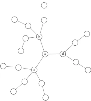
2.3. Multinode Centrality.Apart from computing the centrality of individual graph nodes, one can deﬁne and quantify also the centrality of sets of nodes (see Figure 1). Multinode centrality analyses have already been performed for diﬀerent types of ecological networks including food webs [26] and habitat networks [27].

The most central multinode sets ofn= 1to 4 nodes were identiﬁed for the 27 food webs, according to two diﬀerent aspects of key player selection. First, how to best fragment (disrupt) the network by removing n key nodes (the

“negative” version of the key player problem; KPP-Neg) and second, how to best send a message out fromnnodes of the network to others (the “positive” version; KPP-Pos, see [15]). For KPP-Neg, we determined the most central node sets considering binary (F) and distance-weighted (FR) fragmentation centrality. For KPP-Pos, we determined the most central node sets considering binary m-reach centrality (Mm) and distance-weighted (DR) reachability withm= 1, 2 and 3 steps (M1, M2, and M3, respectively).

Each of the four multinode centrality measures were computed forn= 1to 4 nodes (n= 1is clearly single-node).

Multinode key sets were calculated using Pyntacle, our high-performance network analysis tool.

2.4. Nestedness.The nestedness of presence-absence ecological data [28] has a rich literature with well-developed methods ([29, 30]; for software, see [31]). The nestedness approach has also been extended to ecological interactions in binary networks [32, 33]. Here, we study the nestedness of ecological interaction networks in a very diﬀerent way (see [15, 20, 25]), quantifying the set–subset relationships of central nodes in a network.

We calculated the nestedness of central node sets (i.e., the overlap among the sets of size n= 1to 4) using the Nrow metric [34]. Nrow is the average percentage of nodes from smaller sets that are contained in larger sets, taking all possible pairs of sets. For example, for the food webdemp au, the M2 key player sets for n= 1to 4 nodes were {0} forn= 1, {0 2} for n= 2, {0 68 76} for n= 3, and {76 18 37 66} for n= 4. Forn= 1andn= 2, there is perfect overlap. Forn= 1 and n= 3, there is partial overlap, since the smaller set (n= 1) is a subset of the larger one (n= 3). For n= 2 and n= 4, there is no overlap, since the two sets have no common elements. Averaging all the 6 overlaps, we have Nrow = 47.22, which is the nestedness value for M2 in the demp au food web (see the species identities for this food web in Discussion). The same was done for the remaining centralities (F, FR, M2, M3, and DR) and for all food webs.

2.5. Statistical Analysis.We compared the 9 topological properties of the 27 food webs with their 6 nestedness metrics by Spearman correlation, because most topological properties were not normally distributed. We considered only correlations of 0.60 and above (as well as−0.60 and below). Corre- lations were calculated in R 3.3.0 [35].

3. Results

3.1. Network Metrics. The studied macroscopic network parameters are presented in Table 1. The smallest and the largest networks, in terms of the number of nodes, were the cat(N= 48) and thecarpinteriafood webs (N= 128), respectively. Depending on the various actual numbers of links (L), connectance ranged from C= 0 06 (aka a, cow17, martins, narr, andtroy) toC= 0 16(demp su). Average degree ranged from avD = 4 (aka b,cow17, andnarr) to avD = 18.72 (carpinteria). Diameter ranged from d= 4 (black, cow17, german, healy, andstony) tod= 7(cow1), and the average shortest path length ranged from avSPL = 2.19 (carpinteria) to avSPL = 2.9 (cow1). The average clustering coeﬃcient ranged from avCC = 0.02 (cat, kyeb, sutton sp, and sutton su) to avCC = 0.25 (carpinteria), and the weighted clustering coeﬃ- cient ranged from wCC = 0 (broad,sutton sp, andsutton su) to wCC = 0.25 (carpinteria). Finally, distance-based fragmentation ranged from DF = 0.48 (carpinteria and demp su) to DF = 0.6 (troy).

3.2. Nestedness.Our question was if topology has any significant effect on the nestedness of keystone species complexes in the studied 27 food webs. Between 9 topological properties and 6 nestedness metrics for each food web, we analysed 54 correlations. Only 4 of them were significant (shown in Figure 2), and in each of these M2 was the nestedness index (F, FR, DR, M1, and M3 did not show any significant correlation). M2 correlated positively with DF and avSPL and

b

a

c

d

Figure1: Toy network illustrating the nonnested centrality of node sets. The number of nodes reachable from nodesa,b,c, anddin two steps (m= 2) equals 11, 9, 9, and 7, respectively. Thus, nodeahas the highestm-reach centrality in the network. Yet, from the (a,d) set of nodes only 12 and from the (a,b) or (a,c) set of nodes only 13, while from the (b,c) set of nodes, 14 other nodes are reachable in two steps. Thus, the (b,c) set is more central than the other sets, based on reachability. The highest centrality node (a) is not a subset of the highest centrality set of two nodes (b,c).

(4)

negatively withCand avD (N,L,d, avCC, and wCC did not show any signiﬁcant correlation).

The four signiﬁcant correlations are between M2 and DF (rho = 0.681;p= 0 0009), M2 andC (rho =−0.678;

p= 0 001), M2 and avD (rho =−0.637; p= 0 00035), and M2 and avSPL (rho = 0.605; p= 0 00084). All of them are strongly signiﬁcant.

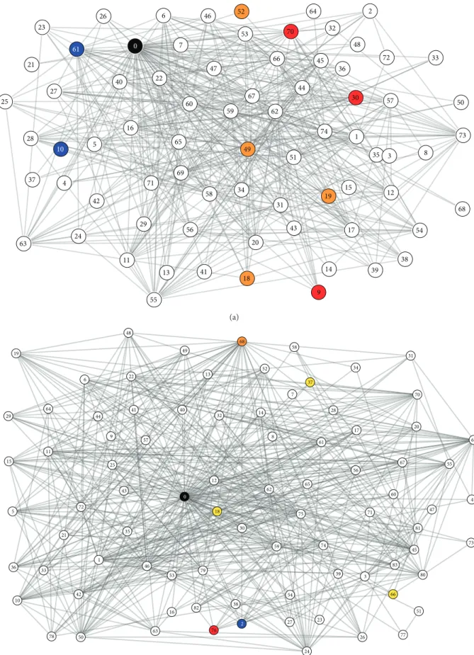
Only a few topological features can be used as a proxy for assessing the nestedness of central node sets, but most of these show quite strong correlations. Our results suggest that in networks where shortest paths are shorter and density is higher, nestedness is lower, so systems-based conservation can be less predictive and efficient. One example is the Sutton tussock grassland in springtime (Figure 3(a), Supplementary Material (available here)). Here, the single most central organism in the network isunidentifiable detritus(#0, black in Figure 3(a)). The most central pair is the diatomCocconeis sp. and the larvae of the riffle beetleHydora nitida(#10 and

#61, blue). The group of the three most central network positions is the red alga Audouinella sp., the diatomNavicula

avenacea, and the caddisfly Pycnocentrodes spp. (#9, #30, and #70, red). The four most central organisms are the alga Epithemia zebra, the diatomEunotiaspp., thefishflyArchi- cauliodes diversus, and Chironomid type “Diamesid blond”

(#18, #19, #49, and #52, orange). Hence, the increasing core of key organisms is perfectly unnested (M2 = 0, up to 4 groups). Accordingly, DF is low (0.51), C is high (0.14), avD is high (10.49), and avSPL is small (2.39). Apart from the single-node core (n= 1), the larger cores (n> 1) are always composed of both plants (e.g., diatoms) and animals (e.g., caddisﬂy).

On the contrary, in less connected and less compact networks, nestedness is higher, so a multispecies view fairly reinforce the results of single-species analyses. One example is the Dempsters tussock grassland in autumn (Figure 3(b), Supplementary Material). Here, the single most central organism in the network isunidentiﬁable detritus(#0, black).

The most central pair is unidentifiable detritus and terrestrial invertebrates (#2, blue). The group of the three most central network positions is unidentifiable detritus, Table1: Topological properties and nestedness of multinode centrality sets for 27 food webs. The topological properties include the number of nodes (N), the number of edges (L), diameter (d), average degree (avD), average shortest path length (avSPL), connectance (C), average clustering coefficient (avCC), weighted clustering coefficient (wCC), and distance-based fragmentation (DF). Nestedness is always calculated for sets ofn= 1to 4 nodes, based on fragmentation (F), distance-based fragmentation (FR), weighted reachability (DR), and binarym-reach form= 1(M1), 2 (M2), and 3 (M3) steps.

Web N L d avD avSPL C avCC wCC DF F DR FR M1 M2 M3

aka a 84 221 5 5.26 2.72 0.06 0.04 0.01 0.58 100 100 80.56 100 77.78 0

aka b 54 108 5 4 2.6 0.07 0.1 0.03 0.56 100 100 94.44 91.67 77.78 0

ber 77 232 5 6.03 2.63 0.08 0.03 0.01 0.57 94.44 100 100 86.11 38.89 5.56

black 85 366 4 8.61 2.45 0.1 0.04 0.03 0.53 100 94.44 77.78 100 41.67 5.56

broad 94 559 6 11.89 2.47 0.13 0.03 0 0.52 100 100 94.44 61.11 5.56 0

cant 108 693 5 12.83 2.37 0.12 0.04 0.01 0.52 100 100 100 100 8.33 16.67

carpinteria 128 1198 5 18.72 2.19 0.15 0.25 0.25 0.48 100 36.11 86.11 30.56 72.22 16.67

cat 48 107 5 4.46 2.42 0.09 0.02 0.01 0.53 100 86.11 100 77.78 33.33 0

cow1 58 118 7 4.07 2.9 0.07 0.11 0.06 0.59 100 91.67 100 100 50 0

cow17 71 142 4 4 2.73 0.06 0.15 0.04 0.59 100 100 55.56 100 72.22 0

demp au 83 410 6 9.88 2.47 0.12 0.03 0.01 0.53 50 100 27.78 100 47.22 0

demp sp 93 535 5 11.51 2.47 0.12 0.04 0.01 0.53 100 69.44 72.22 63.89 8.33 0

demp su 107 918 5 17.16 2.21 0.16 0.09 0.06 0.48 100 100 100 94.44 5.56 16.67

german 84 347 4 8.26 2.58 0.1 0.07 0.05 0.55 100 100 100 94.44 27.78 0

healy 95 603 4 12.69 2.3 0.13 0.07 0.03 0.5 91.67 100 100 94.44 16.67 0

kyeb 98 616 5 12.57 2.4 0.13 0.02 0.02 0.52 100 47.22 83.33 66.67 22.22 0

lilkye 78 372 5 9.54 2.49 0.12 0.07 0.02 0.53 91.67 100 94.44 100 41.67 8.33

martins 104 311 5 5.98 2.65 0.06 0.11 0.04 0.58 100 91.67 66.67 91.67 72.22 5.56

narr 71 142 5 4 2.55 0.06 0.07 0.02 0.57 100 100 94.44 100 77.78 0

north 78 228 5 5.85 2.54 0.07 0.12 0.04 0.55 100 100 100 100 5.56 8.33

powder 78 252 6 6.46 2.58 0.08 0.06 0.01 0.56 100 61.11 91.67 77.78 38.89 0

stony 112 824 4 14.71 2.35 0.13 0.07 0.02 0.51 100 100 86.11 100 16.67 8.33

sutton au 80 331 6 8.28 2.59 0.1 0.03 0.01 0.55 100 100 100 94.44 25 0

sutton sp 74 388 5 10.49 2.39 0.14 0.02 0 0.51 100 100 100 100 0 8.33

sutton su 86 417 5 9.7 2.34 0.11 0.02 0 0.51 100 58.33 94.44 66.67 16.67 0

troy 76 170 6 4.47 2.87 0.06 0.05 0.03 0.6 100 100 91.67 94.44 77.78 11.11

ven 65 184 5 5.66 2.57 0.09 0.06 0.03 0.56 94.44 100 100 100 41.67 0

(5)

and the caddisﬂies Olinga feredayi, and Tiphobiosis sp.

(#68 in orange and #76 in red). The four most central organisms are Tiphobiosis sp., alga Epithemia zebra (#18, yellow), another algaSpirogyra sp. (#37, yellow), and a mayﬂy Nesameletus ornatus(#66 yellow). Here, the composition of the core is a little bit more nested (M2 = 47.22) and, accordingly, DF is somewhat higher (0.53),C is lower (0.12), avD is a little lower (9.88), and avSPL is longer (2.47).

Supplementary Material show the nestedness patterns for each food web. The numbers are the codes for species, and these are generally not comparable for diﬀerent networks.

However, node #0 is almost always unidentifiable detritus (or some similarly large aggregated group, e.g., terrestrial invertebrate remains). In many networks, this is part of the key player complexes. Biologically speaking, this is an arte- fact: the detritus is clearly a well-connected component of food webs. Only other species in the key player complexes can be biologically interpreted. It is also noted thatUnidenti- fiable detritus, even if it is frequently the key group forn= 1, is frequently missing from larger key player sets (e.g., for n= 4 in thedemp au food web). So, even if it dominates the network structure in itself, its position is not significant anymore if we think in terms of a larger network core.

Apart from the large aggregated groups typically being in the centre of the network, the four organisms that can be in the key position also in single-species cores (n= 1) are the diatom Fragilaria vaucheriae (#19 in the broad food web), the shore crab Hemigrapsus oregonensis (#45 in the

carpinteria food web), the mayﬂy Deleatidium spp. (#34 in thenorthfood web), and the diatomRhoicosphenia cur- vata (#16 in the powder food web). Hemigrapsus appears in all of the four studied key player sets in the carpinteria food web (n= 1, 2, 3, 4).

Some communities are described by several versions of the food web (e.g., seasonal versions likedemp au,demp sp, and demp su). In some cases, these versions diﬀer a lot in nestedness (dempand sutton), while in other cases, there is only a small diﬀerence between the versions (akaandcow).

4. Discussion

The dynamical behaviour of complex ecological systems can be dominated by a few critically important components.

Finding these could dramatically increase our understanding, the predictability of models, and the efficiency of management efforts. We studied a comparable set of empirical food webs and identified the structurally most importantnnodes in them. Whether these small sets were nested was correlated to some topological properties of these networks.

Network features inﬂuencing nestedness can be regarded as topological constraints on the predictability and eﬃciency of management and systems-based conservation. It remains unclear to us how M2 and M3 can be negatively and positively correlated with avD, respectively.

We need to much better understand the biology of the key groups and the ecology of nested vs. nonnested

0 20 40 60 80

0.48 0.50 0.52 0.54 0.56 0.58 0.60

M2

DF

(a)

0 20 40 60 80

0.06 0.08 0.10 0.12 0.14 0.16

M2

C

(b)

0 20 40 60 80

5 10 15

M2

avD

(c)

0 20 40 60 80

2.2 2.3 2.4 2.5 2.6 2.7 2.8 2.9

M2

avSPL

(d)

Figure2: Signiﬁcant correlations between topological properties and reachability. DF (a; rho = 0.681; p= 0 0009), C (b; rho =−0.678;

p= 0 001), avD (c; rho =−0.637;p= 0 00035), and avSPL (d; rho = 0.605;p= 0 00084) versus M2. All of them are strongly signiﬁcant.

(6)

59

74 67

66

44

51 62

49

70

48

64 2

45 32

40 22

21

60 47 27

53 61

6

7 23

26 52

0

46

1 35 3

57

72 33

8 36

73 30 50

65 16

5 25

28 10

42

63

4

24 37

43 54

15 34 19

17

68 12

31

20

55 69

11

41 56 71

13

58

29

9 14 39 18

38

(a)

41 40

32 14

57 8 6

52

49 58

19

22 13

68 48

29

25 9

15

64

11

44

61 17

67 56

20

69

55 31

37 7

28

70 34

1

10

50 36

78 33

42

65 0

12

30 18 75

62

63

82 53

38 79

16

76 2 46

26 77

27

66

23 54

24

51 21 35

5 72

43

71

4

81 60

73 47

83 39 3

59 74

80 45

(b)

Figure3: The food webs of the Sutton tussock grassland in spring (a;sutton sp) and the Dempster tussock grassland in autumn (b;demp au).

The coloured species are explained in the text.

(7)

communities. If certain groups (e.g., zooplankton and diatoms) appear frequently in the core of food webs, these can be thought to be real keystone species. This is especially important if the core is nested: this means that the particular community is really dominated by a single species. We still know nothing about the kinds of communities (or the set of abiotic factors) that can be associated with nested patterns.

Biologically speaking, this is the most promising future research line.

All of our results are based on a set of 27 empirical food webs in the size range between 48 and 128 trophic groups.

This is the typical size scale for food webs in the literature.

All the webs were described by the same methodological standards, so they are comparable to each other. In order to see if these results are generalizable, research is needed in at least two directions.

First, one wants to see if topological properties scale with network size. For this, much larger networks should be studied—and the topological properties studied here can be more and more relevant and interesting for larger graphs.

The limitation here is that empirical networks are not larger.

Much larger networks (N> 500) could be constructed by dramatically increasing the resolution of trophic groups (e.g., by adding bacteria and replacing trophic groups by biological species), but these networks would not be biologically comparable to the present ones (even if being mathematically more interesting).

Second, the toy network of the same size range can be generated by various algorithms (already in progress), and empirical topologies could be compared to the theoretical distributions. This kind of randomization analysis is fairly straightforward in community ecology; however, it is not easy to see which generative algorithms give the most realistic results (e.g., [36] but see [37]). These studies could reveal if the reported relationships are universal properties of networks in general, or they are speciﬁc to only food webs for some biological (ecological) reasons (Capocefalo et al.

unpublished). If the results are food web-specific, we need to understand the biological reasons. If the results will be shown to be of general nature, conclusions can be drawn also in other fields of research. For example, terrorist networks have been shown to have large average shortest paths and low density [38], properties suggesting that their efficient

“management”is possible—in a security and defence sense.

This paper is of mostly conceptual and methodological nature. We suggest that the search for the cores of ecosystem networks opens several research lines that could massively contribute to systems-based conservation biology and management, with applications ranging from marineﬁsheries to pollination systems.

Data Availability

Data are available at the personal website of the correspond- ing author: https://ferencjordan.webnode.hu/.

Conflicts of Interest

The authors declare no conﬂict of interest.

Funding

FJ was funded by the grant GINOP-2.3.2-15-2016-00057.

FJ and JP were funded by the grant OTKA K 116071.

Acknowledgments

We are grateful to Zsóﬁa Benedek and Marco Scotti for earlier discussions.

Supplementary Materials

Supplementary Material: the M2 nestedness values for each network (m-reach for 2 steps) and the identity of nodes for key player sets (of diﬀerent sizesn) are presented.

(Supplementary Materials)

References

[1] F. Jordán, “Keystone species and food webs,” Philosophical Transactions of the Royal Society B: Biological Sciences, vol. 364, no. 1524, pp. 1733–1741, 2009.

[2] L. S. Mills and D. F. Doak,“The keystone-species concept in ecology and conservation: management and policy must explicitly consider the complexity of interactions in natural systems,”BioScience, vol. 43, no. 4, pp. 219–224, 1993.

[3] R. T. Paine,“A note on trophic complexity and community stability,”The American Naturalist, vol. 103, no. 929, pp. 91– 93, 1969.

[4] M. E. Power, D. Tilman, J. A. Estes et al.,“Challenges in the quest for keystones: identifying keystone species is diﬃcult— but essential to understanding how loss of species will aﬀect ecosystems,”BioScience, vol. 46, no. 8, pp. 609–620, 1996.

[5] E. Estrada,“Characterization of topological keystone species:

local, global and “meso-scale” centralities in food webs,” Ecological Complexity, vol. 4, no. 1-2, pp. 48–57, 2007.

[6] F. Jordán and I. Scheuring, “Network ecology: topological constraints on ecosystem dynamics,”Physics of Life Reviews, vol. 1, no. 3, pp. 139–172, 2004.

[7] S. Allesina and A. Bodini,“Who dominates whom in the ecosystem? Energyﬂow bottlenecks and cascading extinctions,” Journal of Theoretical Biology, vol. 230, no. 3, pp. 351–358, 2004.

[8] J. A. Dunne, R. J. Williams, and N. D. Martinez, “Network structure and biodiversity loss in food webs: robustness increases with connectance,” Ecology Letters, vol. 5, no. 4, pp. 558–567, 2002.

[9] F. Jordan, A. Takacs-Santa, and I. Molnar,“A reliability theoretical quest for keystones,”Oikos, vol. 86, no. 3, pp. 453–462, 1999.

[10] F. Jordán, T. A. Okey, B. Bauer, and S. Libralato,“Identifying important species: linking structure and function in ecological networks,” Ecological Modelling, vol. 216, no. 1, pp. 75–80, 2008.

[11] C. M. Livi, F. Jordán, P. Lecca, and T. A. Okey,“Identifying key species in ecosystems with stochastic sensitivity analysis,”Eco- logical Modelling, vol. 222, no. 14, pp. 2542–2551, 2011.

[12] B. A. Menge, “Indirect eﬀects in marine rocky intertidal interaction webs: patterns and importance,”Ecological Mono- graphs, vol. 65, no. 1, pp. 21–74, 1995.

(8)

[13] U. Brose, E. L. Berlow, and N. D. Martinez,“Scaling up keystone eﬀects from simple to complex ecological networks,”

Ecology Letters, vol. 8, no. 12, pp. 1317–1325, 2005.

[14] S. P. Borgatti, M. G. Everett, and L. C. Freeman,Ucinet for Windows: Software for Social Network Analysis, Analytic Technologies, Nicholasville, KY, USA, 2002.

[15] S. P. Borgatti,“Identifying sets of key players in a social network,”Computational & Mathematical Organization Theory, vol. 12, no. 1, pp. 21–34, 2006.

[16] J. Pereira and F. Jordán,“Multi-node selection of patches for protecting habitat connectivity: fragmentation versus reachability,”Ecological Indicators, vol. 81, pp. 192–200, 2017.

[17] J. Pereira, S. Saura, and F. Jordán,“Single-node vs. multi-node centrality in landscape graph analysis: key habitat patches and their protection for 20 bird species in NE Spain,”Methods in Ecology and Evolution, vol. 8, no. 11, pp. 1458–1467, 2017.

[18] G. C. Daily, P. R. Ehrlich, and N. M. Haddad, “Double keystone bird in a keystone species complex,”Proceedings of the National Academy of Sciences of the United States of Amer- ica, vol. 90, no. 2, pp. 592–594, 1993.

[19] R. M. May, J. R. Beddington, C. W. Clark, S. J. Holt, and R. M. Laws,“Management of multispeciesﬁsheries,”Science, vol. 205, no. 4403, pp. 267–277, 1979.

[20] M. Ortiz, R. Levins, L. Campos et al., “Identifying keystone trophic groups in benthic ecosystems: implications forﬁsher- ies management,”Ecological Indicators, vol. 25, pp. 133–140, 2013.

[21] M. Ortiz, F. Rodriguez-Zaragoza, B. Hermosillo-Nuñez, and F. Jordán, “Control strategy scenarios for the alien lionﬁsh Pterois volitans in Chinchorro Bank (Mexican Caribbean):

based on semi-quantitative loop analysis,”PLoS One, vol. 10, no. 6, article e0130261, 2015.

[22] M. Ortiz, B. Hermosillo-Nuñez, J. González, F. Rodríguez- Zaragoza, I. Gómez, and F. Jordán, “Quantifying keystone species complexes: ecosystem-based conservation management in the King George Island (Antarctic Peninsula),”Eco- logical Indicators, vol. 81, pp. 453–460, 2017.

[23] R. Albert, H. Jeong, and A. L. Barabasi, “Error and attack tolerance of complex networks,” Nature, vol. 406, no. 6794, pp. 378–382, 2000.

[24] H. Jeong, S. P. Mason, A. L. Barabási, and Z. N. Oltvai,

“Lethality and centrality in protein networks,” Nature, vol. 411, no. 6833, pp. 41-42, 2001.

[25] Z. Benedek, F. Jordán, and A. Báldi, “Topological keystone species complexes in ecological interaction networks,” Com- munity Ecology, vol. 8, no. 1, pp. 1–7, 2007.

[26] J. González, M. Ortiz, F. Rodríguez-Zaragoza, and R. E.

Ulanowicz, “Assessment of long-term changes of ecosystem indexes in Tongoy Bay (SE Paciﬁc coast): based on trophic network analysis,”Ecological Indicators, vol. 69, pp. 390–399, 2016.

[27] L. Rubio, Ö. Bodin, L. Brotons, and S. Saura,“Connectivity conservation priorities for individual patches evaluated in the present landscape: how durable and eﬀective are they in the long term?,”Ecography, vol. 38, no. 8, pp. 782–791, 2015.

[28] J. Podani and D. Schmera,“A new conceptual and methodological framework for exploring and explaining pattern in presence–absence data,” Oikos, vol. 120, no. 11, pp. 1625– 1638, 2011.

[29] W. Atmar and B. D. Patterson,The Nestedness Temperature Calculator: A Visual Basic Programme, Including 294

Presence-Absence Matrices, AICS Research, University Park, NM, and The Field Museum, Chicago, IL, USA, 1995.

[30] J. Podani, C. Ricotta, and D. Schmera, “A general framework for analyzing beta diversity, nestedness and related community-level phenomena based on abundance data,”

Ecological Complexity, vol. 15, pp. 52–61, 2013.

[31] W. An and Y. Liu,“Keyplayer: locating key players in social networks. R package version 1.0.3,”May 2016, https://CRAN.

R-project.org/package=keyplayer.

[32] M. A. Fortuna, D. B. Stouﬀer, J. M. Olesen et al.,“Nestedness versus modularity in ecological networks: two sides of the same coin?,” Journal of Animal Ecology, vol. 79, no. 4, pp. 811–817, 2010.

[33] J. Podani, F. Jordán, and D. Schmera, “A new approach to exploring architecture of bipartite (interaction) ecological networks,” Journal of Complex Networks, vol. 2, no. 2, pp. 168–186, 2014.

[34] M. Almeida-Neto, P. Guimarães, P. R. Guimarães Jr., R. D.

Loyola, and W. Ulrich, “A consistent metric for nestedness analysis in ecological systems: reconciling concept and mea- surement,”Oikos, vol. 117, no. 8, pp. 1227–1239, 2008.

[35] R Core Team,R: A Language and Environment for Statistical Computing, R Foundation for Statistical Computing, Vienna, Austria, 2016, https://www.R-project.org/.

[36] R. J. Williams and N. D. Martinez,“Simple rules yield complex food webs,”Nature, vol. 404, no. 6774, pp. 180–183, 2000.

[37] J. W. Fox, “Current food web models cannot explain the overall topological structure of observed food webs,” Oikos, vol. 115, no. 1, pp. 97–109, 2006.

[38] V. E. Krebs,“Mapping networks of terrorist cells,” Connec- tions, vol. 24, no. 3, pp. 43–52, 2001.

(9)

Hindawi

www.hindawi.com Volume 2018

Mathematics

^{Journal of}

Hindawi

Mathematical Problems in Engineering Applied Mathematics

Hindawi

Probability and Statistics

Hindawi

Mathematical PhysicsAdvances in

Complex Analysis

^{Journal of}

Hindawi

Optimization

^{Journal of}

Hindawi

Engineering Mathematics

International Journal of

Hindawi

Operations Research

Journal of

Hindawi

Function Spaces

Abstract and Applied Analysis

Hindawi

International Journal of Mathematics and Mathematical Sciences

Hindawi

Hindawi Publishing Corporation

http://www.hindawi.com Volume 2013

Hindawi www.hindawi.com

World Journal

Volume 2018

Hindawi

www.hindawi.com Volume 2018Volume 2018

Numerical Analysis Numerical Analysis Numerical Analysis Numerical Analysis Numerical Analysis Numerical Analysis Numerical Analysis Numerical Analysis Numerical Analysis Numerical Analysis Numerical Analysis

Numerical AnalysisAdvances inAdvances in Discrete Dynamics in Nature and Society

Hindawi

Hindawi www.hindawi.com

Differential Equations

Volume 2018 Hindawi

Decision Sciences

Hindawi

Analysis

Hindawi

Stochastic Analysis

Food Web Topology and Nested Keystone Species Complexes

Research Article