Environmental drivers of plant community assembly in Isla de los Estados at Southern Atlantic Ocean

(1)

dOi: 10.1556/168.2018.19.1.4

Introduction

Effective management decisions for biodiversity conservation are essential for maintaining human well-being and ecosystem processes (Rands et al. 2010), mainly considering the future climate change scenarios (Hole et al. 2009).

Climate change greatly influences forest ecosystem types around the World, and the chain of causalities is currently quite difficult to understand (Luque et al. 2011). As part of biodiversity protection and climate change mitigation, the efforts in conservation science must consider the organization of biodiversity at the landscape level to design robust protected area networks or the understanding processes that maintain species diversity in the natural environments (Socolar

et al. 2016). The current protected area network throughout the World contains a biased sample of biodiversity, usually located in remote places or areas that are unsuitable for com- mercial activities (Margules and Pressey 2000). For example, in Southern Patagonia most of the conservation strategies have been developed under politically-driven agreements between Chile and Argentina, rather than taking into account specific conservation strategies determined by ecological needs (Martínez Pastur et al. 2016a). Consequently, the protected areas are dominated by Nothofagus pumilio forests (Luque et al. 2011), thus neglecting most of the regional biodiversity which is poorly represented in the natural protection areas (e.g., N. antarctica forests, shrublands and natural grasslands, Martínez-Harms and Gajardo 2008, Martínez Pastur et al. 2016a).

Environmental drivers of plant community assembly in Isla de los Estados at Southern Atlantic Ocean

A. Huertas Herrera

^1,2

, M. V. Lencinas

¹

and G. Martínez Pastur

¹

1Laboratorio de Recursos Agroforestales (CADIC CONICET). Houssay 200 (9410) Ushuaia, Tierra del Fuego, Argentina

2Corresponding author. Email: ahuertasherrera@cadic-conicet.gob.ar

Keywords: Biodiversity, Conservation, Forests, Multi-Scale, Open-Lands, Southern Hemisphere.

Abstract: The comprehensive assessment of environmental gradients influencing species assemblages is important for imple- menting new conservation strategies under climate change. This study aims to determine the multi-scale effect of altitudinal and longitudinal gradients as drivers of richness and plant community assembly in mountain landscapes of Isla de los Estados (Argentina) to identify areas with greater conservation value in Southern Patagonia. We chose three fjords across the island that extends from West to East and we categorized landscapes into four ecosystem types according to their vegetation type (forests and open-lands) and elevation (lower lands, 0-100 m.a.s.l. and upper lands, 300-400 m.a.s.l.). Forest structure, soil cover (woody debris, rocky outcrop and bare soil) and vegetation cover (vascular and non-vascular), including richness and growth- forms (trees, shrubs, prostrate and erect herbs, tussock and rhizomatous grasses, ferns and inferior plants) were measured in 60 sampling areas (3 fjords × 2 vegetation types × 2 elevations × 5 replicates). ANOVAs and multivariate methods were used to analyse heterogeneity in forest structure, plant richness, and life-form. In addition, species richness and the Simpson’s diversity index were calculated to understand plant assembly at multiple-scales (α, β and γ). Our results showed that environmental gradients (altitudinal and longitudinal) are more important drivers of change of ecosystem type than forest spatial structure.

Furthermore, forest structure significantly varied with altitudinal and longitudinal gradients affecting most of the studied variables. A greater similarity (in richness and cover) between open-lands of lower and higher elevations was detected, as well as between forests. Fjords showed a West-East gradient, where the western and center fjords were more closely related to each other than to the eastern fjord. A multi-scale diversity approach may play central role in improving our understanding the main environmental drivers of richness and plant community assembly in these forests, both theoretical and empirical, and may be used to identify the spatial scale at which ecosystem types have greater conservation value. This study indicates that for southern forest conservation at regional level, efforts must cover all environmental gradients, including the different vegetation types to assure ful conservation of all the species assemblages.

Abbreviations: BA–Basal Area, BS–Bare Soil, DBH–Breast Height, DCA–Detrended Correspondence Analyses, DEN–

Tree Density, DH–Dominant Height, EH–Erect Herbs, F–Ferns, FH–Forest High Elevation, FL–Forest Low Elevation, HI–

Homogeneity Index, IP–Inferior Plants, MRPP–Multi-Response Permutation Procedure, OH–Open High Elevation, OL–Open Low Elevation, PH–Prostrate Herbs, RC–Rocky Outcrop, RG–Rhizomatous Grasses, SH–Shrubs, TG–Tussock Grasses, TR–

Trees, WD–Woody Debris.

Nomenclature: We followed plant species nomenclature by Moore (1983). See Appendix Table A for the complete codes of recorded species.

(2)

36 Huertas Herrera et al.

Most of the natural reserves focus their protection tar- gets on forests, despite the other associated environments, which were demonstrated to include unique species of different taxonomic groups (Lencinas et al. 2005, 2008a,b). In addition, biodiversity values can greatly vary across the landscape for the same vegetation type, where significant changes can be observed in the Tierra del Fuego archipelago (e.g., Nothofagus forests) (Martínez Pastur et al. 2016b, 2017). In this sense, effective conservation strategies can be developed using multi-scale approaches (e.g., α, β and γ diversity measurements), as well as studies that improve the understanding the response of species assemblages to environmental gradients. More recent attention has focused on these biodiversity measurements at different spatial levels to analyze drivers of change in richness and community assemblages and to inform global conservation policy. The PREDICTS project (Projecting Responses of Ecological Diversity in Changing Terrestrial Systems) is a biodiversity database, serving as a good example of how these multi-scale measurements can be used to better understand natural or land use- related human impacts on community assembly at multiple scales (Newbold et al. 2016, Hudson et al. 2017). Another example is the PEBANPA Network in Southern Patagonia (Argentina), where biological and environmental indicators from permanent and semi-permanent plots provide guidance for researchers and decision makers regarding ecology, conservation biology and sustainable land management at different spatial scales (Peri et al. 2016).

For this, to improve understanding the factors that influence species coexistence, we propose as the objective of this study the assessment of environmental drivers of plant community assembly in Isla de los Estados at the Southern Atlantic Ocean (Argentina). Specifically, we want to answer the following questions: (i) have richness and plant community assemblage changed with ecosystem types and with the altitudinal and longitudinal gradients? and (ii) is it possible to identify areas with greater conservation value among the distinctive vegetation types and fjords within the reserve using diversity indices using a multi-scale approach? Since understory plants are important indicators of biotic assemblages of different taxa over a regional gradient (Lencinas et al. 2008a, Mestre et al. 2017), this work might contrib- ute to a new scientific panorama on globally interconnected processes in plant community ecology, temperate ecosystem biogeography, nature conservation and the effect of global climate change on mountain plant communities.

Methods Study area

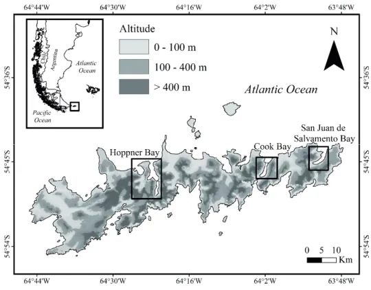
The study was conducted at Isla de los Estados Natural Reserve (Administración de Parques Nacionales, Argentina) located in the eastern portion of the Tierra del Fuego archipelago (54°38’ to 54°54’ SL, 64°45’ to 63°47’ WL (Fig. 1).

We choose this study area to minimize human impact, since it is an isolated big island in the Southern Atlantic Ocean. This

island presents unique conservation characteristics, offering a wide variety of natural settings from West to East with ac- cessible fjords. These environments include steep slopes with an altitudinal gradient from sea level to the mountain tree- line, which allowed us to test ecological responses in short distances (Körner 2007). The island covers about 520 km² of extremely rugged and mountainous landscape, with a peak elevation of 800 m.a.s.l. (Ponce and Fernández 2014). Deeply indented and dissected fjords, bays and harbors make up the coastline (Dudley and Crow 1983), and sheltered lowland ecosystems are predominantly colonized by evergreen forest, whereas open-land areas exposed to strong winds were com- posed by Magellanic moorland formations (Moore 1983). The major soil type is inceptisol (Cruzate and Panigatti 2007), the ground at low and intermediate elevations is extremely wet, whereas the mountain peak ridges consist almost entirely of rocky promontories and mineral soil. The climate is predominantly sub-polar (Kottek et al. 2006), and strongly influenced by persistent low pressure that develops near the Antarctic (Ponce et al. 2017). Monthly mean temperature varied between 8.3°C (summer) and 3.3°C (winter), a mean annual precipitation reached 1450 mm.year^-1 with strong frequent winds of 95-140 km.h^-1 (Dudley and Crow 1983).

Sampling design and data acquisition

Data collection was conducted during November 2014 with a vessel at 3 fjords that extend from West to East di- rection: (i) Port Hoppner Bay (West fjord), Port Cook Bay (Center fjord) and Port San Juan de Salvamento Bay (East fjord). Fjords were chosen for their accessibility, and because they were the most typical geographic areas with mountain landscapes in the Island (Körner et al. 2011). Landscapes in each fjord were categorized into four ecosystem types according to their vegetation type (forests and open-lands) and elevation in lower lands (0-100 m.a.s.l.) and upper lands (300- 400 m.a.s.l.), resulting in four treatments: open-lands (OL) and forests (FL) at lower elevations with greater influence of sea closeness, and open-lands (OH) and forests (FH) at higher elevations close to the tree-line with greater exposure to extreme climate and mountain environments. We defined these altitudinal thresholds based on Barrera et al. (2000) and Kreps et al. (2012).

A total of 60 sampling areas were selected (3 fjords × 2 vegetation types × 2 elevations × 5 replicates) according to their homogeneity, accessibility and size (patches up to 5 ha each). Each site was established at least 500 m from the oth- ers. In the centre of each patch, one plot was established for sampling vegetation and forest structure. Vegetation census considering vascular plants (dicots, monocots, pteridophytes) was made at the species level in 1 ha at each plot, following the taxonomy proposed by Moore (1983), while non-vascular plants (mosses, liverworts) and lichens were considered as a different group. We defined the species growth-forms, based on their visible morphology and following Dale et al. (2002) and Faber-Langendoen et al. (2014), as trees (TR), shrubs (SH), prostrate herbs (PH), erect herbs (EH), tussock grasses (TG), rhizomatous grasses (RG) and ferns (F), and in the case

(3)

Environmental gradients as drivers of richness and plant community assemblage 37

of mosses, liverworts and lichens as “inferior plants” (IP).

Both the vascular and non-vascular vegetation cover was estimated using a modified Braun-Blanquet scale (Clarke 1986, Lencinas et al. 2011). In addition, cover of bare soil (including litter) (BS), rocky outcrop (RC) and woody debris (WD) were also estimated.

Forest structure was characterized using two different methods: in FL plots the point sampling method (Bitterlich 1984) using a Criterion RD-1000 (Laser Technology, USA) with a variable BAF (basal area factor between 6 and 9) was employed, while in FH fixed plots of 200 m² (transects of 50 m × 4 m) were used due to the presence of krummholz trees. Each tree was identified at species level, and its diameter at breast height (DBH) was measured with a forest caliper. Also, dominant height (DH) was measured using a Trupulse 360 (Laser Technology, USA). From these data we calculated basal area (BA), tree density (DEN) and homogeneity index (HI) as the ratio between total BA of the plot and BA of Nothofagus betuloides, because it is the major representative species of the evergreen forests in the Island.

Herbarium specimens were deposited in the Laboratorio de Recursos Agroforestales (CADIC-CONICET) at Ushuaia city (Argentina).

Data analyses

Floristic representativeness of our samples were determined using species accumulation curves with the EstimateS 9.0 (Colwell et al. 2012) software (Appendix: Figure A1), while the frequency of occurrence of each species (total number of sample plots in which a species occurred) considering vegetation types and fjords allowed us to determine the importance and variation of each species at treatment and land-

scape level. Total understory cover partitioned by its growth- forms (TR, SH, PH, EH, TG, RG, F, IP), as well as soil cover (BS, RC, WD), were analysed through multifactorial analyses of variance (ANOVA) considering ecosystem types (OL, FL, OH, FH) and fjords (West, Center, East) as main factors.

Forest structure (DH, BA, DEN, DBH, HI) was analysed through multifactorial ANOVAs considering forested ecosystem types (FL, FH) and fjords (West, Center, East) as main factors. For some analyses, growth-forms were grouped for a better interpretation of data as follows: prostrate and erect herbs (PEH), tussock and rhizomatous grasses (TRG) and ferns and inferior plants (FIP). Inferior plants and ferns were grouped since they often carpeted together the floor´s ecosystem types. In all cases, Shapiro-Wilk and Levene methods were used to test normality and homogeneity, respectively.

When the assumptions were not met, these response variables were log-transformed to normalize their distributions, but non-transformed average data are shown (just two variables in Table 1). Finally, we used the post-hoc Tukey test (p < 0.05) to separate mean significant values.

Multivariate analyses were conducted with plant species cover to analyse ecosystem types (OL, FL, OH, FH) and fjords (West, Center, East): (i) cluster analyses were performed using Ward’s method with Euclidean distance to link the plant composition assemblage to the studied gradients; and (ii) detrended correspondence analyses (DCA) were performed to assess the heterogeneity in species composition. For multivariate analyses, species cover matrices were used according to the necessary steps of each of analyses (e.g., the ordering of rows and columns of the matrices). In the case of clusters, two matrices were created separately for ecosystem types and fjords, while for DCA we used a single main matrix of species and two secondary matrices (ecosystem types and fjords). For

23 Figure 1. Study area at Isla de los Estados: Hoppner Bay (west fjord), Cook Bay (center fjord) and San Juan de Salvamento Bay (east fjord). Gray scale represents elevation (m.a.s.l.).

Figure 1. Study area at Isla de los Estados:

Hoppner Bay (west fjord), Cook Bay (center fjord) and San Juan de Salvamento Bay (east fjord). Gray scale represents elevation (m.a.s.l.).

(4)

DCA, we first tested the data by detrending the segments to decide which ordination method must be used (linear or unimodal), where the obtained gradient length value was larger than four standard deviations (SD) indicating the convenience of the unimodal method (ter Braak and Šmilauer 2015). DCA was chosen because it provides simultaneous analyses of species and sampling units (Hill and Gauch 1980), allowing the examination of ecological interrelationships between them in a single-step analysis (Ludwig and Reynolds 1988). Analyses were based on species relative cover matrix without down- weighting for rare species and with axis rescaling (Hill 1979).

The statistical differences between ecosystem types and fjords (sample groups) were tested using the Multi-Response Permutation Procedure (MRPP) with Sorensen (Bray-Curtis) distance measure (Peck 2010). All statistical analyses were performed using PC-Ord (McCune and Mefford 1999).

Finally, ecosystem types and fjords were characterized through their alpha (α), beta (β) and gamma (γ) diversity in order to understand the understory plant assemblages both at local and landscape level. We consider that α characterizes each treatment at each studied area, β quantifies the differentiation degree of treatments along the studied environmental gradients, and γ results from the differentiation between α and β (Whittaker 1972). We measured diversity based on (i) the specific richness (number of species, S) and (ii) the species contribution (Simpson dominance index, SDI) (Moreno 2001). For diversity measurements based on S: (i) α was calculated as the mean of species richness recorded in the plots of each ecosystem type or fjord; (ii) β was estimated as S_jq_j(S_T – S_j),

where q_j is the proportional weight of each treatment j (as- signing a weight of 25% to each ecosystem type and a weight of 33.3% to each fjord), ST is the total number of species sur- veyed in all the plots of each treatment, and S_j is the number of species registered in treatment j; and (iii) γ was computed as

g = α + β.

For diversity measurements based on SDI: (i) α was calculated as

SDI = 1 – λ,

being λ = Sp_i, with p_i as the proportional abundance of species; (ii) β was calculated as

S_jqjl_j – Sipi;

and (iii) γ was calculated as g = α + β.

Results

Dominant height, basal area and DBH significantly varied with the elevation, decreasing in magnitude when the elevation increases (Table 1). Basal area and DBH also presented significant differences among fjords, with increasing trends of both values from West to East. Tree density and the homogeneity index presented significant differences neither in elevation nor in fjords. Interactions between factors were only

significant for the basal area (p = 0.031) since in all fjords the forests at lower elevations (FL) had similar values but the forests at higher elevations (FH) were significantly different only in the East (Appendix: Figure A2).

Members of the flora recorded by sampling in the Island were native and included 22 dicots (3 trees, 9 shrubs, 8 prostrate herbs, 2 erect herbs), 8 monocots (2 prostrate herbs, 1 erect herb, 2 tussock grasses, 3 rhizomatous grasses) and 5 ferns (Appendix: Table A). The most frequent plants during the entire sampling period included two trees (Nothofagus betuloides and Drimys winteri), two shrubs (Chiliotrichum diffusum and Pernettya mucronata) and one prostrate herb (Luzuriaga marginata). The species accumulation curves showed that sampling was sufficient enough to capture most of the richness of the studied ecosystem types and fjords, which was higher in OL and West fjord (Appendix: Figure A).

Plant and soil cover variables significantly changed among the ecosystem types (Table 2). At lower elevations, forests (FL) were present on 7.0% of bare soil due to the higher overstory canopy closure, and at higher elevations open- lands (OH) were mainly present on rocky outcrops (10.1%) and 1.0% bare soil due to wind exposure and climatic limi- tations for full vegetation development. As was expected, woody debris was higher inside the forests (4.0%) than in open-lands. Interactions between ecosystem type × fjord were significant for bare soil (p = 0.023) since the forests at lower elevations had significantly higher values in the East than West and Center fjords. For rocky outcrop (p = 0.003) interaction occurred since the open-lands at higher elevations presented significantly higher values in the East than the other treatments. No interactions were detected for woody debris (Appendix: Figure A2).

Total vegetation cover varied with elevation, being greater in open lands than in forests at lower elevations (OL vs.

FL) and, contrariwise, it was greater in forests than in open- lands at higher elevations (FH vs. OH). Also, the assemblage of growth-forms varied with the considered ecosystem type.

As was expected, grasses (19-27%) were higher in open- lands, however regeneration from trees was also higher here (17-23%) showing a potential advantage of the forests in these open environments. Contrarily, as was expected, shrubs were greater in the forests (35% in FL and 52% in FH) than in open-lands (11-20%). Ferns were greater in FL (31%) than in the other environments (14-19%). Finally, herbs showed significant differences (p = 0.040) but the post-hoc test did not detect differences among the treatments (open-lands > forests). Plant and soil cover also significantly changed among fjords for most of the studied variables. Rocky outcrop was greater in East, while woody debris was lower in the West.

In consequence, total vegetation was lower in the East with a different assemblage of growth-forms across the fjords. Tree regeneration was greater in the East, herbs were greater in the Center, and ferns and inferior plants were greater in the West.

Interactions between factors were significant for trees (p = 0.008) due to their higher values at the open-lands in the East fjord than other fjords. Similar patterns of trees in relation to elevation were observed in forests at higher elevations in the West. Thus, non-significant differences between ecosystem

~

2 2

~

(5)

types occurred only in the Center. Interactions in shrubs (p = 0.005) occurred by significantly higher values in the forest at high elevation than in another ecosystem type in the Center.

For herbs (p = 0.011), interaction took place due to significantly higher cover in open-lands of lower and higher elevations than in forest ecosystems in the Center. Interactions in total plant cover (p = 0.048) occurred due to open-lands at lower and forests at higher elevations had significantly lower values in East than the other treatments. No interactions were detected for woody debris, ferns and inferior plants and rhizomatous grasses.

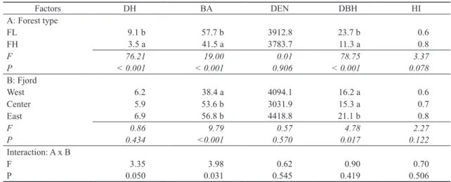
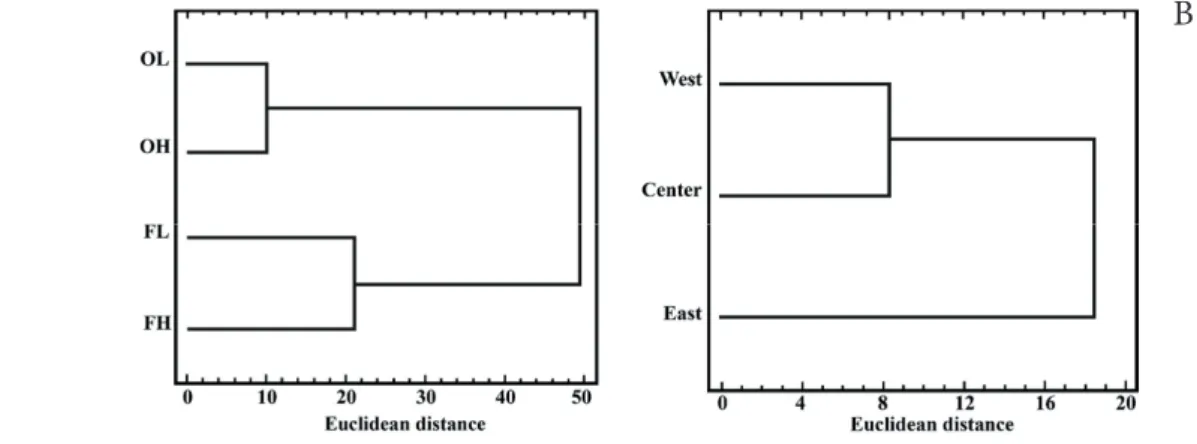
Multivariate analyses presented the same patterns that were described before (Figs 2-3). Cluster analyses showed a greater similarity between open-lands of lower and higher elevations, as well as forests of lower and higher elevations. Fjords showed a West-East gradient, where West and Center fjords were more closely related than East fjord. DCA showed a similar pattern with significant differences (total variance = 4.683, axis 1 with an eigenvalue of 0.732 and a length of gradient of 5.440, and axis 2 with an eigenvalue of 0.388 and a gradient length of 2.890), where open-lands presented more similarities among the sampling points than the forests. MRPP analysis showed significant differences among Table 1. Two-way ANOVAs for forest structure considering tree overstory dominant height (DH, m), basal area (BA, m² ha^-1), tree density (DEN, n ha^-1), diameter at breast height (DBH, cm), and homogeneity index (HI, %) of evergreen forests, where forest type (A) and fjords (B) were the main factors, and A × B their interactions. DH and DBH were ln(Y) transformed prior to analyses, but not transformed data are shown.

Factors DH BA DEN DBH HI

A: Forest type

FL 9.1 b 57.7 b 3912.8 23.7 b 0.6

FH 3.5 a 41.5 a 3783.7 11.3 a 0.8

F 76.21 19.00 0.01 78.75 3.37

P < 0.001 < 0.001 0.906 < 0.001 0.078

B: Fjord

West 6.2 38.4 a 4094.1 16.2 a 0.6

Center 5.9 53.6 b 3031.9 15.3 a 0.7

East 6.9 56.8 b 4418.8 21.1 b 0.8

F 0.86 9.79 0.57 4.78 2.27

P 0.434 <0.001 0.570 0.017 0.122

Interaction: A x B

F 3.35 3.98 0.62 0.90 0.70

P 0.050 0.031 0.545 0.419 0.506

F = Fisher test, p = significance level. Values followed by different letters were significantly different with Tukey test at p < 0.05. Forest types: FL = forest low elevation, FH = forest high elevation.

Table 2. Two-way ANOVAs for floor cover (%) (BS = bare soil, RC = rocky outcrop, and WD = woody debris) and cover plants (%) classified according their growth-forms (TR = trees, SH = shrubs, PEH = prostrate and erect herbs, TRG = tussock and rhizomatous grasses, FIP = ferns and inferior plants, and TOTAL = total plant cover), where ecosystem type (A) and fjords (B) were the main factors, and A x B their interactions.

Factors BS RC WD TR SH PEH TRG FIP TOTAL

A: Ecosystem type

OL 0.0 a 1.4 a 0.0 a 16.6 ab 20.0 a 21.2 26.9 c 13.8 a 98.5 b

FL 6.7 c 0.7 a 4.5 b 9.7 a 35.1 b 11.7 0.1 a 31.3 b 88.1 a

OH 1.1 ab 10.1 b 0.2 a 23.3 b 10.7 a 20.2 19.1 bc 15.4 a 88.6 a

FH 0.0 a 0.1 a 3.9 b 11.2 a 52.1 c 7.8 6.3 ab 18.7 a 96.1 ab

F 3.81 9.18 14.22 3.92 20.44 2.97 12.98 7.63 4.67

p 0.015 < 0.001 < 0.001 0.014 < 0.001 0.040 < 0.001 < 0.001 0.006

B: Fjord

West 0.1 2.4 ab 0.9 a 15.8 ab 26.8 12.8 ab 13.5 27.7 b 96.6 b

Center 1.5 0.8 a 2.8 b 8.7 a 32.7 23.2 b 12.5 17.8 a 94.9 b

East 4.3 6.0 b 2.7 ab 21.7 b 29.0 9.8 a 13.2 14.0 a 87.0 a

F 2.12 4.03 3.74 5.20 0.75 4.57 0.03 7.91 5.82

p 0.131 0.024 0.031 0.009 0.479 0.015 0.977 0.001 0.005

Interaction: A x B

F 2.72 3.94 1.64 3.30 3.58 3.14 1.54 1.81 2.31

p 0.023 0.003 0.156 0.008 0.005 0.011 0.186 0.115 0.048

F = Fisher test, p = significance level. Values followed by different letters were significantly different with Tukey test at p <0.05.

Ecosystem types: OL = open low elevation, FL = forest low elevation, OH = open high elevation, FH = forest high elevation.

(6)

all the defined vegetation groups (T = –21.260, A = 0.195, p

< 0.001). The pairwise comparisons indicated that all ecosystem type combinations were distinct: OL vs. FL (T = –16.442, A = 0.211, p = 0.000); OL vs. OH (T = –12.502, A = 0.157, p

= 0.000); OL vs. FH (T = –2.637, A = 0.034, p = 0.020); FL vs. OH (T= –9.351, A = 0.095, p = 0.000), FL vs. FH (T = –15.262, A = 0.182, p = 0.000); OH vs. FH (T = –11.691, A

= 0.141, p = 0.000). Fjords presented their plots intermixed,

Figure 3. Detrended correspondence analyses (DCA) comparing assemblages of plant species based on the scores of species (A), and samples at different ecosystem types (B) (OL = open low elevation, FL = forest low elevation, OH = open high elevation, FH = forest high elevation) and fjords (C) (West, Center and East). For species codes, see Appendix: Table A.

25

Axis 1 (eigenvalue = 0.732)

Ecosystem type OLFL OHFH

NOBE NOAN

DRWI BEIL

BOGU CHDI

ESSE

EMRU

GAAN MADI

PEMU PEPU

ACPU

ASPU CADI AZLY

DRMU

DRUN GUMA

GULA

LUMA

RUGE

COLE

PEMA SEAC

COPI

FECO CAAL

HIRE MAGR

BLPE BLMA

GRMA HYTO

POMO Axis 1 (eigenvalue = 0.732)

Fjord WestCenter East

Figure 3. Detrended correspondence analyses (DCA) comparing assemblages of plants species based on the scores of species (A), and samples at different ecosystem types (B) (OL = open low elevation, FL = forest low elevation, OH = open high elevation, FH = forest high elevation) and fjords (C) (West, Center and East).

Species code were presented in Appendix Table A.

26 Figure 2. Cluster analyses using Ward’s method of linkage with Euclidean distance: (A) plant cover species (%) among ecosystem types (OL = open low elevation, FL = forest low elevation, OH = open high elevation, FH = forest high elevation), and (B) fjords (West, Center and East).

Figure 2. Cluster analyses using Ward’s method of linkage with Euclidean distance: (A) plant cover species (%) among ecosystem types (OL = open low elevation, FL = forest low elevation, OH = open high elevation, FH = forest high elevation), and (B) fjords (West, Center and East).

A B

C

(7)

however, some species have their centroid in DCA indicating that their distribution is linked to a particular location (Fig.

3A). Axis 1 from left to right indicates a gradient from West to East, e.g., in the West fjord: Carpha alpina, Cortaderia pilosa, Drosera uniflora, Gaultheria antarctica, Grammitis magellanica, Maytenus disticha and Rubus geoides; in the Centre fjord: Acaena pumila and Caltha dioneifolia; and in the East fjord: Azorella lycopodioides and Festuca contracta.

MRPP analysis showed significant differences among all the fjords (T = –5.345, A = 0.037, p < 0.001). Likewise, MRPP confirmed significant statistical differences between all fjords pairwise comparisons: West vs. Center (T = –2.290, A = 0.019, p = 0.033); West vs. East (T = –3.981, A = 0.027, p = 0.002); Center vs. East (T = –4.715, A = 0.038, p = 0.001).

Gamma plant species diversity for the entire study area reached 37 species (Simpson index = 0.88). Open-lands at lower elevations maintain the greatest (76% of the species) and forest at lower elevations the lowest richness (49% of the species), with fjords decreasing in diversity from West to East (78% to 65% of the species) for all the studied environments (Table 3). Beta plant species richness showed that 40% of the species were shared for the overall study, being greater in the open-lands than in forests (6 vs. 10-12 species).

Discussion

Richness and plant community assemblage changed with ecosystem types and environmental gradients

Forest structure of the study area corresponded to native old-growth stands without previous management, where the southern Patagonian N. betuloides was the dominant species.

Multi-scale analyses revealed that forest structure varied with altitudinal and longitudinal gradients, thus affecting the main variables related to forest structure. At the ecosystem type level (OL, FL, OH, FH), we found that dominant height, basal

area and DBH significantly varied with the elevation, decreasing in magnitude when the elevation increases. In the fjords (West, Center, East) the relationship between forest structure and longitudinal gradients produced significant changes in basal area and DBH, whith increasing trends of both variables from West to East. Similarly, recent research in Tierra del Fuego suggested that these multi-scale differences are associated with elevation or location of the stands in the landscape (Martínez Pastur et al. 2012, Mestre et al. 2017), which can be also related to climate at the regional level (Frangi et al. 2005, Lencinas et al. 2011).

For temperate forests, it is well-known that forest structure makes a notable contribution to dynamics, composition, and biodiversity (Tilman 1994, Frangi et al. 2005, Barbier et al. 2008, Martínez Pastur et al. 2013).

Previous work on southern temperate forests have shown how these structural variables were related to temperature, radiation, and soil moisture, which are critical factors that af- fect natural regeneration dynamics (Heinemann et al. 2000, Martínez Pastur et al. 2011), decomposition and natural cy- cles (Barrera et al. 2000), as well as biodiversity (Lencinas et al. 2008a, 2008b, 2011). In the temperate forests of the Northern hemisphere, previous studies have shown that the forest structure and natural gradients are more related to the distinctiveness of understorey composition than to tree specific forest types (Bonari et al. 2017), where the assemblages of the understory plants might relate both to the main environmental gradients and the particular tree species functional traits (Terwei et al. 2016). However, functional diversity traits may also influence the community assembly. For example, Kumordzi et al. (2015) found that the successional age and species richness of forest understorey vegetation communities are linked to species coexistence through their effects on within and between species functional diversity. In our work, both altitudinal and longitudinal gradients had a significant effect on plant assembly in ecosystem types with same topog- raphy, climate, soil properties and water regime. This find- Table 3. Plant species diversity (α, β and γ) for ecosystem types and fjords. Diversity values are shown as number of species and Simpson index (values in parenthesis) was calculated within each ecosystem type across the fjords.

Diversity Treatment n Fjord

Total

West Center East

α

Ecosystem type

OL 5 22 (0.84) 20 (0.87) 14 (0.84) 28 (0.88)

FL 5 14 (0.87) 14 (0.81) 11 (0.83) 18 (0.86)

OH 5 14 (0.86) 15 (0.74) 12 (0.70) 22 (0.87)

FH 5 18 (0.89) 13 (0.79) 16 (0.88) 22 (0.90)

β

Pairwise comparisons

OL-FL 10 7 (0.05) 8 (0.06) 3 (0.06) 10 (0.05)

OL-FH 10 6 (0.04) 6 (0.07) 4 (0.03) 10 (0.03)

OL-OH 10 5 (0.01) 3 (0.02) 7 (0.08) 10 (0.01)

FL-FH 10 6 (0.01) 4 (0.07) 5 (0.03) 6 (0.01)

FL-OH 10 6 (0.04) 8 (0.11) 8 (0.11) 12 (0.05)

FH-OH 10 6 (0.03) 5 (0.10) 7 (0.08) 15 (0.04)

Overall 20 12 (0.01) 11 (0.01) 11 (0.01) 15 (0.01)

γ Total number of species 60 29 (0.86) 26 (0.80) 24 (0.81) 37 (0.88)

Ecosystem types: OL = open low elevation, FL = forest low elevation, OH = open high elevation, FH = forest high elevation.

(8)

ing differs from Barbier et al.’s (2008) who suggested that understory vegetation is directly affected by the forest types in temperate and boreal forests. Nevertheless, since there was no human impact and the entire flora was native, we found that the environmental gradients (altitudinal and longitudinal) are more important drivers of change of ecosystem type plant assemblages than forest spatial structuring.

It is interesting for forest ecology that interaction between the environmental factors determined ecosystem’s plant richness and life form. In our study, this interaction indicated a potential forest encroachment into open lands along a longitudinal gradient. Thus, although not directly apparent, this forest advance may be important evidence of climate change influence on forest ecosystem types at the southern hemisphere. Based on the results of Terrestrial net primary production (NPP) and southern climate scenarios described by Zhao and Running (2010) and Kreps et al. (2012), a possible expla- nation for this (the potential advance of the forests) might be that temperatures and higher levels of precipitation associated with biodiversity assemblage are adequate for the forest in the southern hemisphere, allowing trees to grow better than other plant life-forms (PH, EH, TG, RG, F). In addition, N.

betuloides (main tree component of these forests) is a moder- ately tolerant tree species due to its colonization abilities and natural dynamics, and to large quantities of sapling and seed- ling plants in the understory (Promis et al. 2010, Martínez Pastur et al. 2012). In other temperate forests it has been reported that global temperatures already have a negative impact on woody species, with elevated mortality and declining reproduction leading to regional decline and dieback events worldwide (Jump et al. 2009). In our study, we found that southern temperate forests actually might benefit from spatial variability in resources along mountain gradients, which may also substantially facilitate their advance in the open environments. Therefore, this spatial pattern evidenced the role of environmental gradients on plant assemblage change and demonstrate how important it is to safeguard the connections between forest and their associated environments.

Is it possible to identify areas with greater conservation value?

It is known that different ecological processes might determine plant biodiversity at different spatial scales (Crawley and Harral 2001). Different authors highlight that southern Nothofagus forests rarely constitute large, continuous exten- sions and simultaneously exhibit marked temporal and spatial variability in resources (Lencinas et al. 2008a, Martinez Pastur et al. 2013). Since species occurring only in specific areas acquire greater ecological and conservation importance, while those with less habitat specialization lose relevance for landscape-scale management, a great part of land needs to be integrated into sustainable models to ensuring the preserva- tion of the associated environments (Lencinas et al. 2008a, 2011). However, several studies consider biodiversity at global and regional scale, thus the spatial associations with landscape factors at other scales remain seldom explored (Martínez Pastur et al. 2016a,b). This can be considered as a

gap in our knowledge about the distribution of plant species linked to the multi-scale effect of environmental variables (Martínez Pastur et al. 2016a). This has also been an incom- plete understanding of natural balance with undesirable con- sequences for biological conservation overseas (Hudson et al.

2017). All ecosystems together guarantee the diversity that gives more resilience to the whole system (Peri et al. 2016, Hudson et al. 2017), because forests do not perform all their ecological functions as just a group of trees (Martínez Pastur et al. 2017).

In our study, the environmental gradient influenced over the species assemblages covering their natural range. The multi-scale analysis has shown that at α-level, forest plant diversity differed from open land-associated environments along the altitudinal gradient, where the open lands contain a much larger number of plant communities than the forests.

Influenced by rocky outcrops and woody debris, at this α- level we found evidence for unique plant assemblages and growth-forms across the fjords: (i) assembly in open-lands of lower and higher elevations, and (ii) assembly in forests of lower and higher elevation (species assemblages are shown by the multivariate analysis). Besides, some species presented clear preferences for alpine environments (e.g., Bolax gummifera, Escallonia serrata, and Azorella lycopo- dioides). These results are consistent with Martínez Pastur et al. (2016b, 2017) who observed significant changes in the forest species assemblages of Tierra del Fuego. Nevertheless, when we considered the degree of differentiation (β), plant species diversity showed that less than 50% of the species were shared for the overall study. This β may be explained by the high dominance of inferior plants in all ecosystem types, as reported by (Lencinas et al. 2011) for the temperate forest in Tierra del Fuego. At the γ-level, the relationship between studied factors (elevation vs. longitude) revealed that differences among fjords occurred at vegetation type level (forest and open-lands). Furthermore, the γ result provided not only a trend of fewer species from West to East across the studied ecosystems but also indicated that there is a zone of concen- tration of unique species assemblages and greatest complex- ity of growth-forms. Based on this analysis, the East fjord may be the area (comprising all plant assembles) to have the greatest conservation value among the different vegetation types and fjords. itt

These results reinforce the idea that southern forest conservation at regional level efforts must include all associated open environment to assure the conservation of all the species.

For southern Patagonia (Argentina) we already know that national conservation strategy creates a particular dichotomy between nature and society (Luque et al. 2011, Gamondès Moyano et al. 2016). Protection was regarding marginal unproductive forests, and biodiversity values are not included in the strategies, e.g., national legislation (26331/07) and the Argentine protected area network. For a balance with natural resources, forest managers and policymaking should take into account the conservation of associated forest environments (Lencinas et al. 2008a, Lindenmayer et al. 2008). We propose to use a multi-scale diversity approach as a decision tool for these conservation strategies at regional level. This may solve

(9)

the problem of non-representativeness of plant species across protected areas at southernmost ecosystems, and improve the understanding of the implications of the climate change at multiple-scale levels of plant species assemblage.

Conclusions

We found enough evidence that environmental gradients were the main driver of change of plant species assemblages in the temperate forest and open-lands ecosystems of Isla de los Estados. Each ecosystem type, as small as it may look when compared to the forest covers, it actually has a huge importance for plant richness due to the part it plays in regional diversity. Multi-scale diversity approach may play a central role in improving the understanding of main environmental drivers of richness and plant community assemblage in these forests, both theoretical and empirical, and make possible to identify the spatial scale at which ecosystems type greater conservation value. Our results show that some plants only occurs in special environments or are exclusive to some location. In addition, climate change may be benefiting for the forest advance along mountain landscape in the southern hemisphere. Conservation efforts at the regional level in the southern forest must include all associated open environment to assure the conservation of all the species.

Acknowledgements: We want to especially thank F. Guerrero and Quixote Expeditions (http://www.quixote-expeditions.

com) for their invaluable support for the field work. Also, we want to thanks to S. Kather and B. Díaz for the collaboration for the data taking and plant identification.

References

Barbier, S., F. Gosselin and P. Balandier. 2008. Influence of tree species on understory vegetation diversity and mechanisms in- volved. A critical review for temperate and boreal forests. For.

Ecol. Manage. 254:1–15.

Barrera, M., J. Frangi., L. Richter, M. Perdomo and L. Pinedo. 2000.

Structural and functional changes in Nothofagus pumilio forest along an altitudinal gradient in Tierra del Fuego, Argentina. J.

Veg. Sci. 11:179–188.

Bitterlich, W. 1984. The Relascope Idea. Relative Measurements in Forestry. Commonwealth Agricultural Bureaux, London, UK.

Bonari, G., A.T. Acosta and C. Angiolini. 2017. Mediterranean coast- al pine forest stands: Understorey distinctiveness or not? For.

Ecol. Manage. 391:19–28.

Clarke, R. 1986. The Handbook of Ecological Monitoring. Claredon Press, Oxford.

Colwell, R.K., A. Chao, N.J. Gotelli, S-Y. Lin, C.X. Mao, R. Chazdon and J.T. Longino. 2012. Models and estimators linking individ- ual-based and sample-based rarefaction, extrapolation and com- parison of assemblages. J. Plant Ecol. 5:3–21.

Crawley, M. and J. Harral. 2001. Scale dependence in plant biodiversity. Sci. 291:864–868.

Cruzate, G.A. and J.L. Panigatti. 2007. Suelos y ambientes Isla Grande de Tierra del Fuego-Argentina. ArgenINTA, Buenos Aires, Argentina.

Dale, V.H., S.C. Beyeler and B. Jackson. 2002. Understory vegetation indicators of anthropogenic disturbance in longleaf pine forests at Fort Benning, Georgia, USA. Ecol. Indic. 1:155–170.

Dudley, T.R. and G.E. Crow. 1983. A contribution to the flora and vegetation of Isla de los Estados (Staten Island), Tierra del Fuego, Argentina. In: B. Parker (ed.), Antarctic Research Series.

Terrestrial Biology II, vol.37. American Geophysical Union, Washington DC, pp. 1–26.

Faber-Langendoen, D., T. Keeler-Wolf, D. Meidinger, D. Tart, B.

Hoagland, C. Josse, G. Navarro, S. Ponomarenko, J.-P. Saucier and A. Weakley. 2014. EcoVeg: a new approach to vegetation description and classification. Ecol. Monogr. 84:533–561.

Frangi, J.L., M.D. Barrera, J. Puig de Fábregas, P.F. Yapura, A.M.

Arambarri and L. Richter. 2005. Ecología de los bosques de Tierra del Fuego. In: M.F. Arturi, J.L. Frangi and J.F. Goya (eds.), Ecología y manejo de bosques nativos de Argentina.

Editorial Universidad Nacional de La Plata, La Plata, pp. 1–88.

Gamondès Moyano, I., R.K. Morgan and G. Martínez Pastur.

2016. Reshaping forest management in Southern Patagonia: A Qualitative Assessment. J. Sustain. For. 35:37–59.

Heinemann, K., T.H. Kitzberger and T.H. Veblen. 2000. Influences of gap microheterogeneity on the regeneration of Nothofagus pumilio in a xeric old-growth forest of northwestern Patagonia, Argentina. Can. J. For. Res. 30:25–31.

Hill, M.O. 1979. DECORANA-A FORTRAN program for detrended correspondence analysis and reciprocal averaging. Ecology and Systematics, New York.

Hill, M.O. and H.G. Gauch Jr. 1980. Detrended correspondence analysis: An improved ordination technique. Vegetatio 42:47–58.

Hole, D.G., S.G. Willis, D.J. Pain, L.D. Fishpool, S.H. Butchart, Y.C.

Collingham, C. Rahbek and B. Huntley. 2009. Projected impacts of climate change on a continent-wide protected area network.

Ecol. Lett. 12:420–431.

Hudson, L.N., T. Newbold, S. Contu, S.L. Hill et al. 2017. The database of the PREDICTS (Projecting Responses of Ecological Diversity in Changing Terrestrial Systems) project. Ecol. Evol.

7:145–188.

Jump, A.S., Cs. Mátyás, J. Peñuelas. 2009. The altitude-for-latitude disparity in the range retractions of woody species. Trends Ecol.

Evol. 24:694–701.

Körner, C. 2007. The use of ‘altitude’ in ecological research. Trends Ecol. Evol. 22:569–574.

Körner, C., J. Paulsen and E.M. Spehn. 2011. A definition of moun- tains and their bioclimatic belts for global comparisons of biodiversity data. Alp. Bot. 121:73–78.

Kottek, M., J. Grieser, C. Beck, B. Rudolf and F. Rubel. 2006.

World map of the Köppen-Geiger climate classification updated.

Meteorol Z. 15:259–263.

Kreps, G., G. Martínez Pastur and P.L. Peri. 2012. Cambio climáti- co en Patagonia Sur: Escenarios futuros en el manejo de los recursos naturales. Ed. Instituto Nacional de Tecnología Agropecuaria, Buenos Aires, Argentina.

Kumordzi, B.B., F. Bello, G.T. Freschet, L. Bagousse-Pinguet, J.

Lepš and D.A. Wardle. 2015. Linkage of plant trait space to successional age and species richness in boreal forest understorey vegetation. J. Ecol. 103:1610–1620.

Lencinas, M.V., G. Martínez Pastur, M. Medina and C. Busso. 2005.

Richness and density of birds in timber Nothofagus pumilio forests and their unproductive associated environments. Biodiv.

Conserv. 14:2299–2320.

Lencinas, M.V., G. Martínez Pastur, P. Rivero and C. Busso. 2008a.

Conservation value of timber quality versus associated non-tim-

(10)

ber quality stands for understory diversity in Nothofagus forests.

Biodiv. Conserv. 17:2579–2597.

Lencinas, M.V., G. Martínez Pastur, C.B. Anderson and C. Busso.

2008b. The value of timber quality forests for insect conservation on Tierra del Fuego Island compared to associated non-timber quality stands. J. Insect Conserv. 12:461–475.

Lencinas, M.V., G. Martínez Pastur, E. Gallo and M. Cellini. 2011.

Alternative silvicultural practices with variable retention to improve understory plant diversity conservation in southern Patagonian forests. For. Ecol. Manage. 262:1236–1250.

Lindenmayer, D., R.J. Hobbs, R. Montague-Drake, J. Alexandra et al.

2008. A checklist for ecological management of landscapes for conservation. Ecol. Lett. 11:78–91.

Ludwig, J.A. and J.F. Reynolds. 1988. Statistical Ecology: A Primer of Methods and Computing. Wiley, New York.

Luque, S., G. Martínez Pastur, C. Echeverría and M.J. Pacha. 2011.

Overview of biodiversity loss in South America: A landscape perspective for sustainable forest management and conservation in temperate forests. In: C. Li, R. Lafortezza and J. Chen (eds.), Landscape Ecology and Forest Management: Challenges and Solutions in a Changing Globe. HEP-Springer, Amsterdam, Holland. pp. 352–379.

Margules, C.R. and R.L. Pressey. 2000. Systematic conservation planning. Nature 405:243–253.

Martínez-Harms, M.J. and R. Gajardo. 2008. Ecosystem value in the Western Patagonia protected areas. J. Nat. Conserv. 16:72–87.

Martínez Pastur, G., P.L. Peri, J.M. Cellini, M.V. Lencinas, M.

Barrera and H. Ivancich. 2011. Canopy structure analysis for es- timating forest regeneration dynamics and growth in Nothofagus pumilio forests. Ann. For. Sci. 68:587–594.

Martínez Pastur, G., C. Jordán, R. Soler, M.V. Lencinas, H. Ivancich and G. Kreps. 2012. Landscape and microenvironmental con- ditions influence over regeneration dynamics in old-growth Nothofagus betuloides Southern Patagonian forests. Plant.

Biosyst. 146:201–213.

Martínez Pastur, G., P.L. Peri, M.V. Lencinas, J.M. Cellini, M.D.

Barrera, R. Soler, H. Ivancich et al. 2013. La producción for- estal y la conservación de la biodiversidad en los bosques de Nothofagus en Tierra del Fuego y Patagonia Sur. Silvicultura para los bosques de Chile, Valdivia.

Martínez Pastur, G., P.L. Peri, M.V. Lencinas, M. García-Llorente and B. Martín-López. 2016a. Spatial patterns of cultural ecosystem services provision in Southern Patagonia. Landsc. Ecol.

31:383–399.

Martínez Pastur, G., P.L. Peri, R.M. Soler, S. Schindler and M.V.

Lencinas. 2016b. Biodiversity potential of Nothofagus forests in Tierra del Fuego (Argentina): Tool proposal for regional conservation planning. Biodiv. Conserv. 25:1843–1862.

Martínez Pastur, G., P.L. Peri, A. Huertas Herrera, S. Schindler, R.

Díaz-Delgado, M.V. Lencinas and R. Soler. 2017. Linking potential biodiversity and three ecosystem services in silvopastoral managed forests landscapes of Tierra del Fuego, Argentina. Int.

J. Biodiv. Sci. Ecosyst. Serv. Manage. 13:1–11.

McCune, B. and M.J. Mefford. 1999. Multivariate Analysis of Ecological Data, Version 4.0, MjM software. Gleneden Beach, Oregon.

Mestre, L., M. Toro Manríquez, R. Soler, A. Huertas Herrera, G.

Martínez Pastur and M.V. Lencinas. 2017. The influence of canopy-layer composition on understory plant diversity in southern temperate forests. For. Ecosyst. 4:6.

Moore, D. 1983. Flora of Tierra del Fuego. Anthony Nelson, London, UK.

Moreno, C.E. 2001. Métodos para medir la biodiversidad. M&T- Manuales y Tesis SEA, Zaragoza.

Newbold, T., L.N. Hudson, A.P. Arnell, S. Contu, A. De Palma, S.

Ferrier, S.L. Hill, A.J. Hoskins, I. Lysenko and H.R. Phillips.

2016. Has land use pushed terrestrial biodiversity beyond the planetary boundary? A global assessment. Science 353:288–291.

Peck, J.E. 2010. Multivariate Analysis for Community Ecologists:

Step-by-Step Using PC-ORD. MjM Software Design, Gleneden Beach.

Peri, P.L., M.V. Lencinas, J. Bousson, R. Lasagne, R. Soler, H.

Bahamonde and G. Martínez Pastur. 2016. Biodiversity and ecological long-term plots in Southern Patagonia to support sustainable land management: The case of PEBANPA network. J. Nat.

Conserv. 34:51–64.

Ponce, J.F., A.M. Borromei, B. Menounos and J. Rabassa. 2017.

Late-Holocene and Little Ice Age palaeoenvironmental change inferred from pollen analysis, Isla de los Estados, Argentina.

Quat. Int. 442:26–34.

Ponce, J.F. and M. Fernández. 2014. Climatic and Environmental History of Isla de los Estados, Argentina. Springer, Netherlands.

Promis, A., J. Caldentey and M. Ibarra. 2010. Microclima en el inte- rior de un bosque de Nothofagus pumilio y el efecto de una corta de regeneración. Bosque 31:129–139.

Rands, M.R., W.M. Adams, L. Bennun, S.H. Butchart et al. 2010.

Biodiversity conservation: challenges beyond 2010. Science 329:1298–1303.

Socolar, J.B., J.J. Gilroy, W.E. Kunin and D.P. Edwards. 2016. How should beta-diversity inform biodiversity conservation? Trends Ecol. Evol. 31:67–80.

ter Braak, C.J. and P. Šmilauer. 2015. Topics in constrained and un-Šmilauer. 2015. Topics in constrained and un-. 2015. Topics in constrained and un- constrained ordination. Plant Ecol. 216:683–696.

Terwei, A., S. Zerbe, I. Mölder, P. Annighöfer, H. Kawaletz and C.

Ammer. 2016. Response of floodplain understorey species to environmental gradients and tree invasion: a functional trait perspective. Biol. Invasions 18:2951–2973.

Tilman, D. 1994. Competition and biodiversity in spatially structured habitats. Ecology 75:2–16.

Whittaker, R.H. 1972. Evolution and measurement of species diversity. Taxon 21:213–251.

Zhao, M. and S.W. Running. 2010. Drought-induced reduction in global terrestrial net primary production from 2000 through 2009. Science 329:940–943.

Received November 29, 2017 Revised January 2, 2018 Accepted March 1, 2018 Appendix

Table A1. Frequency of occurrence (%), defined growth- forms, and codes for the sampled vascular plants in the different ecosystem types.

Figure A1. Species accumulation curves for ecosystem types.

Figure A2. ANOVAs interactions.

The file may be downloaded from www.akademiai.com.