Heterogeneity effects in power grid network models

Heterogeneity effects in power grid network models

Géza Ódor and Bálint Hartmann

Centre for Energy Research of the Hungarian Academy of Sciences, P. O. Box 49, H-1525 Budapest, Hungary

(Received 4 April 2018; published 8 August 2018)

We have compared the phase synchronization transition of the second-order Kuramoto model on two- dimensional (2D) lattices and on large, synthetic power grid networks, generated from real data. The latter are weighted, hierarchical modular networks. Due to the inertia the synchronization transitions are of first-order type, characterized by fast relaxation and hysteresis by varying the global coupling parameter K. Finite-size scaling analysis shows that there is no real phase transition in the thermodynamic limit, unlike in the mean-field model. The order parameter and its fluctuations depend on the network size without any real singular behavior. In case of power grids the phase synchronization breaks down at lower global couplings, than in case of 2D lattices of the same sizes, but the hysteresis is much narrower or negligible due to the low connectivity of the graphs. The temporal behavior of desynchronization avalanches after a sudden quench to lowKvalues has been followed and duration distributions with power-law tails have been detected. This suggests rare region effects, caused by frozen disorder, resulting in heavy-tailed distributions, even without a self-organization mechanism as a consequence of a catastrophic drop event in the couplings.

DOI:10.1103/PhysRevE.98.022305 I. INTRODUCTION

Power grids are large complex, heterogeneous dynamical system, built up from nodes of energy suppliers and con- sumers. These units are interconnected by a network that enables energy distribution in a sustainable way. However, unexpected changes may cause failure that can be described by synchronization events, which may propagate through the whole system as an avalanche, causing blackouts of various sizes. As the worst case these can lead to full system desynchronization, lasting for a long time [1]. To avoid these events power grid systems should be designed to be resilient to local instabilities, failures, and disturbances. Studies have shown that valuable insights into the dynamical behavior of power grids can be obtained by theoretical studies that consider models of electrical generators, coupled in network structures, reproducing the topological and electrical interactions of real power grids [2,3].

The so-called second-order Kuramoto model was proposed to describe power grids [4] and a number of studies exists, which focus on the synchronization and stability issues, such as in Refs. [5–14]. This is the generalization of the Kuramoto model [15] with inertia. One of the main consequences of this inertia is that the second-order phase synchronization transition, observed in the mean-field models, turns into a first-order one [16]. However, according to our knowledge, the transition type, if any, in lower dimensions has not been studied. It is well known that discontinuous mean-field phase transitions can turn into continuous one as the consequence of fluctuation effects [17]. Fluctuation effects are enhanced in lower spatial dimensions, so it is an open question what happens on a homogeneous, two-dimensional system. There- fore power grids may become critical, exemplified especially by the scale-free distributions measured on them [18]. This criticality has been attributed to some self-organization (SOC) mechanism [19].

On the other hand, highly heterogeneous, also called disor- dered with respect to the homogeneous, system can experience rare region effects that smear phase transitions [20]. Rare regions, which are locally in another state than the whole, evolve slowly and contribute to the global order parameter and can generate various effects, depending on their relevancy.

They can change a discontinuous transition to a continuous one [21], can generate so-called Griffiths phases (GP) [22] or completely smear the singularity of a critical phase transition.

In case of GP-s critical-like power-law (PL) dynamics appears over an extended control parameter region around the critical point, causing slowly decaying autocorrelations and burstiness [23]. Furthermore, in the GP the susceptibility diverges with the system size. Therefore, we decided to investigate if topological and coupling strength heterogeneities of power grids are strong enough to generate critical dynamics or a GP.

We generated weighted graphs of power grids, which are similar to the real ones and large enough to allow reliable statistical physics analysis, including finite-size scaling. We created networks fromN 10⁶toN 2.3×10⁷nodes and compared the phase synchronization transition results of the second-order Kuramoto model with those of two-dimensional (2D) lattices of similar sizes.

II. MODELS AND METHODS

We have studied the second-order Kuramoto model pro- posed by Ref. [4] to describe network of oscillators with phase θ_i(t):

θ˙i(t)=ωi(t)

˙

ωi(t)=ω_i,0−aθ˙i(t)+ K Ni

j

Aijsin[θi(t)−θj(t)],(1) where N_i is the number of incoming edges of node i, a is the damping parameter describing the power dissipation, and

Kis the global coupling related to the maximum transmitted power between nodes andAij, which is the weighted adjacency matrix of the network, containing admittance elements.

The (quenched) heterogeneity comes into the model in two ways: viaω_i,0s, as intrinsic frequencies of the nodes and via Aij, which describes both the topology and the admittances of the power grid. As for the intrinsic frequencies, we used uncorrelated Gaussian random variables, with the distribution centered around the mean ωi =50 and unit variances to model real AC system, although the results have been found to be invariant for this value. For the damping parameter we assumed:a=1,3.

We have studied three different types of networks:

(i) fully connected to recover mean-field results

(ii) 2D lattices, with periodic boundary conditions simu- lating homogeneous electric power grids

(iii) synthetic hierarchical modular ones, generated ran- domly, following the characteristics of real electric power grids.

A. Description of the synthetic power grids

Analysis of the electric power system often requires the use of network models to a certain extent; however, the specific examinations largely affect the nature and the quantity of networks that are necessary to produce authentic results. In certain cases, it is sufficient to perform analysis on one or only a few networks. These usually represent either high-voltage (HV) transmission and subtransmission systems or medium- and low-voltage (MV and LV) distribution systems; the mixed use of these networks for the same scope is rare. In case of HV networks, analysis can be based on network data acquired from utilities and system operators, since the volume of the data is limited in this case, and most of this information is also openly available. This is partly the reason for the over-representation of HV networks in the field of power grid network analysis [24].

In case of MV and LV networks, however, another solution is necessary to perform extensive analysis.

One possible solution is to acquire data of so-called rep- resentative or reference network models (RNM). RNMs are often used tools, when future grid expansion scenarios have to be compared from the perspective of infrastructural needs, maintenance costs, or power losses. Two common methods are used to create such RNMs. The first approach is based on real network data of the utilities; by applying clustering techniques the most typical topological configurations are identified. The literature discusses several methods to create RNMs; a deep and thorough review is presented in Ref. [25]. The disadvan- tage of this method is that it results only a limited number actual networks, which do not provide sufficient variability for our examinations. The second approach is used in case no real network data is available, and synthetic networks are built.

Widely used and known examples for such synthetic networks are the IEEE Bus systems, which are long-time cornerstones of network-related studies in the power engineering field.

The necessity of synthetic networks has been highlighted by several publications during the last couple of years. Reference [26] emphasized in their work that future power engineering problems are in the need of appropriate randomly generated grid networks that have plausible topology and electrical

parameters. They have also concluded that the admittance matrix has peculiar features that follow statistical trends. The generalized random graph model is used to generate synthetic networks in Ref. [27], but the node count of the introduced networks are by magnitudes smaller than it is necessary for our studies. Similar problems are faced with the dual-stage method in Ref. [28], where node count is in the range of thousands. For the examinations shown in present paper, the authors have developed a new power grid network generator algorithm, which has significant differences compared to the existing ones. As these differences are related to the aim of providing a realistic recreation of real power-grid networks, main modeling assumptions and goals are discussed in the following.

The task of the power system is to provide cooperation between power plants, create interconnection on the national and international levels, and to transmit and distribute the produced electricity. To achieve these goals at minimum ecological and economic costs, the structure of power systems has evolved so that transmission and distribution networks have significantly different characteristics. When designing the sample networks for current work, the aim of the authors was to replicate functionality of real power systems, thus those two levels were handled differently. While admittance matrix of the transmission network is based on a real-life example (the Hungarian power system), the matrix of the distribution network is the result of synthetic grid modeling.

The transmission level of a power system has to handle the largest blocks of power, while interconnecting major genera- tors stations and loads of the system. To achieve best overall operating economy or to serve technical objectives best, energy flows in the transmission system can be routed, generally, in any desired direction. The topology of the transmission system tends to obtain a loop structure, which not just provides more path combinations, as no designated flow directions are found, but ensures an increased level of security. Each node of the network can receive power through multiple connections, thus the system is tolerant to single failures [so-called (N−1) criterion].

Considering its current functionality and structure, former subtransmission networks have to be handled similarly to transmission networks, although certain differences are to be noticed. Subtransmission networks are usually designed to have a designated power flow direction from source to sink and have a mixed loop-radial topology. In Hungary, the transmission network mainly consists of 750-, 400-, and 220-kV lines and substations, while the nominal voltage of the former subtransmission level is 120 kV. The security of delivery is increased such that both the 220- to 400-kV and the 120-kV network is meshed and many parallel (double) lines are also operated.

The distribution level of a power system constitutes the finest meshes in the overall network. The circuits are fed from subtransmission level (120 kV) and supply electricity to the small (residential) and medium-sized (small industrial and commercial) customers. The topology of this network is dominantly radial, thus nodes have fewer connections com- pared to the transmission networks. The primary distribution level (20 and 104 kV) is fed directly from the 120-kV or -MV substations. The MV feeders cover wider supply areas and

each feeder supplies multiple distribution transformers. These transformers provide connection between the primary and the secondary distribution level. The latter on is operated at 0.4-kV nominal voltage.

Due to the functional and topological characteristics, the node number of distribution networks is by magnitudes bigger than transmission networks. On one hand, this characteristic makes distribution grids a suitable choice for the examination of synchronization transition of networks. On the other hand, examination of real topologies would require a large collection of electrical and topological data, which is usually not openly available from utility companies, thus synthetic grid modeling is favored to recreate this part of the power system.

As it was shown previously, a number or publications discuss the possibilities of both clustering power grids and creating synthetic topologies for analysis. One of the common weaknesses of these methods is that they dominantly focus on HV and MV networks, which have limited number of nodes, insufficient for our studies. To present a rough comparison, the proportion of the number of HV, MV, and LV nodes in a power system is in the range of 1:100:10000, respectively. The only field, where LV networks are extensively studied, is the area of reference networks models, which are used to determine power losses of the network, but in this case usually only a set of representative networks are created, which is limiting the number of topologies to be examined. In contrast for present paper the authors have generated random power system topologies consisting of a few million nodes. The other main difference between the processed literature and our method is that the present work uses solely weighted graphs, while the cited ones rely mostly on unweighted ones, which ignore valuable information on the behavior of the power system.

Another significant extension of the authors’ model is that transformers are represented as weighted binode connections, instead of the typical choice of handling the two terminals of the transformer as a single node. With this extension the node and connection number of the admittance matrix is increased and the node degree distribution is also affected.

To generate the random topologies, the authors have used an iterative process in MATLAB. The initial step of the process it to set up the transmission and subtransmission levels (lines and transformers) and to mark all 120-kV substations. In the second step a random number is generated to determine the nature of the connected MV network; in Hungary approximately one-third of all MV networks are cable lines (operated on 10 kV) and two-thirds are overhead lines (operated on 20 kV).

It is important to distinguish these voltage levels not only because of different admittance values but also because of their different topological characteristics (line length, transformer nominal power, number of feeders, etc.). After the voltage level is determined, the 120-kV or -MV transformer is created.

Nominal power (and thus admittance) of the unit is selected using the empirical distribution of such units’ nominal powers.

As the next step, length of the MV feeder main and branch lines is calculated, and the position of MV and LV transformers is selected along the lines. Electrical parameters of the lines are also based on empirical distributions and actual per-length line admittances. As the last process of the topology generation, binode connections representing MV/LV transformers are created, and the LV radial network is generated in a similar

FIG. 1. Structural representation of the synthetic networks. Left side: HV; right side: a radial cabinetwork. The highlighted red node connects the two “layers.” The network on the picture has 68 850 nodes and 68 849 edges.

way as it was shown with the MV. In the final step, individual LV consumers are added; this step largely increases the number of nodes with single connection in the network, affecting thus the node degree distribution of the graph representation as well.

B. Analysis of the synthetic power grids

The number of nodes in networks that are generated with the previously described process is approximatelyN = 23 million, which is already sufficient to use for modeling synchronization processes, but computation times are also slowed down significantly. To find the golden mean of network size and computation times, the authors have decided to reduce these networks, while preserving its typical characteristics. As a result, networks with few (1–3) million nodes were generated, using the same iterative process as described before. Network analysis was performed on these networks, the result of which is presented in the following, using three example networks with approximately N =1, 1.5, and 2.5 million nodes. To represent the structure of these networks, Fig. 1 is used an example. The left side of the figure shows the looped HV network, while on the right side the radial network of a HV node is plotted. It can be seen, that the structure of the radial network is similar to a tree, with relatively low node degrees and practically zero clustering coefficient.

10⁰ 10² 10⁴ 10⁶ 10⁸

Number of nodes 0

5 10 15 20 25 30

Node degree

1.5M 1M 2.5M

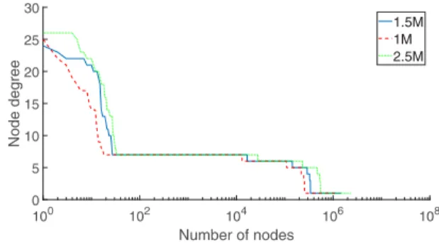
FIG. 2. Node degree distributions of the synthetic power grids generated for 2.5M, 1.5M, and 1M networks (right to left curves).

10⁰ 10² 10⁴ 10⁶ Number of edges

10⁰ 10² 10⁴ 10⁶ 10⁸

Admittances (1/ohm)

1.5M 1M 2.5M

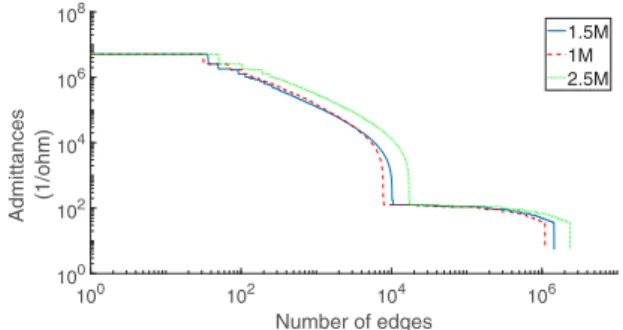
FIG. 3. Admittance distribution of the power grids generated for 2.5M, 1.5M, and 1M networks (right to left curves).

The degree distribution of the networks on Fig.2shows that only a limited number of nodes have high degrees. This is again due to the radial structure of the system, where only looped subnetworks are considered central parts of the network. The high number of nodes withk=5 andk=6 degrees represent LV feeders, where three or four end-users are connected to the same nodes of a radial network. The admittance distribution on Fig.3is composed of a low- and a high-value region, the latter exhibits a tail, which can be fitted linearly for 17.1001/<

Yij <93.0001/. To compare our results with those of the weightless networks we used the normalized admittances as weights:

A_ij =Y_ij/Y_ij, (2) by averaging over the directed edges of the networks.

Further graph measures for four example networks is shown in TableI, including the most important metrics. The average shortest path length is

L= 1

N(N−1)

j=i

d(i, j), (3)

where d(i, j) is the graph (topological) distance between verticesiandj. Considering the clustering coefficient, as it was shown previously, as vast majority of the network (including more than 99.995% of the nodes) has a tree structure, the value of the coefficient is near zero and the small differences are caused by the structure of the central looped subnetworks. Thus clustering coefficients of these subnetworks are included in the table. The subnetworks consist of 37,49,60,and 539 edges, respectively. The different graph measures are calculated, the first one is based on triangle motifs count and the second is based on local clustering. The Watts-Strogatz clustering coefficient [29] of a network ofNnodes is

C^W = 1 N

i

2ni/ki(ki−1), (4)

TABLE I. Power-grids generated and studied.

Network N Edge no. L C C^W

1M 1 098 583 1 098 601 1.7440×10⁶ 0 0

1.5M 1 455 343 1 455 367 1.0457×10⁶ 0.0594 0.0486 2.5M 2 356 331 2 356 360 1.6162×10⁶ 0.0851 0.0586 23M 23 551 140 23 551 254 2.1129×10⁶ 0.0626 0.0741

10⁰ 10¹ 10²

r

10⁻³ 10⁻² 10⁻¹ 10⁰

<Nr>

23M r^1.16(1)

0 0.2 0.4 0.6

1/r 1

1.2 Deff

FIG. 4. Average number of nodes within topological distancer in the 23M graph. Dashed line shows a PL fit for 4< r <20. Inset:

Local slopes defined in Eq. (7).

wheren_idenotes the number of direct links interconnecting the ki nearest neighbors of nodei. An alternative is the “global”

clustering coefficient [30] also called “fraction of transitive triplets,”

C= number of closed triplets

number of connected triplets. (5) An important measure is the topological (graph) dimension D. It is defined by

Nr ∼r^D, (6) whereNris the number of node pairs that are at a topological (also called “chemical”) distance r from each other (i.e., a signal must traverse at leastredges to travel from one node to the other). The topological dimension characterizes how quickly the whole network can be accessed from any of its nodes: The largerD, the more rapidly the number ofrth nearest neighbors expands asrincreases. To measure the dimension of the network we first computed the distances from a seed node to all other nodes by running the breadth-first search algorithm.

Iterating over every possible seed, we counted the number of nodes Nr with graph distance r or less from the seeds and calculated the averages over the trials in case of the largest, 23M network. As Fig.4shows, an initial power law breaks down due to the finite network size. The smallN_rvalues are due to the sparsity and directedness of the graph. We determined the dimension of the network, as defined by the scaling law (6) by attempting a PL fit to the dataNr for the initial ascent.

This suggests a slightly superlinear behavior, increasing with the presence of central nodes.

To see the corrections to scaling we determined the effective exponents ofDas the discretized, logarithmic derivative of (6)

D_eff(D+1/2)= lnNr −lnNr+1

ln(r)−ln(r+1) . (7) These local slopes are shown in the inset of Fig. 4 as the function of 1/rand provide an increasing effective dimension due to the HV nodes, before the finite-size breakdown. A similar analysis for the undirected U.S. HV power grid with

N =4941 nodes [31] results inD >2. That means that this power grid has higher graph dimension than the embedding space due to some extra links. In our case the small number of HV links do not provide such contribution but the other, directed ones, which occur in the distribution subnetworks, dominate the whole topology.

C. Comparison with other synthetic power grids The synthetic networks generated by the authors model is significantly different to other synthetic networks, published in the literature. Such network generation methods are introduced in Refs. [28,32–34]. The model proposed in Ref. [32] was created in order to model HV transmission networks. The topology and the electrical parameters of the network are created using specific random distribution functions, avoiding both topological self-loops and islanded parts. The three-step process uses a predetermined number of nodes, with randomly distributed locations, selects neighboring links of each bus and finally checks whether all nodes are connected. The resulting networks have an average node degree between 2.66 and 3.32, which is in range with real HV topologies with low node number.

Ma et al. [28] presents “dual-stage constructed random graph,” generated by an algorithm in two steps. First a random graph with one connected component is created, then addi- tional edges are added to the spanning tree. The algorithm is tested on four networks; resulting average node degrees are between 2.42 and 2.774.

A random growth model is proposed in Ref. [33] to create synthetic network topologies. A heuristic target func- tion is used for redundancy and cost optimization during the initialization, and an attachment rule during the growth phase. The resulting networks have an average node degree of approximately 2.67, and the degree distribution shows an exponential tail; both are characteristics of HV transmission networks. Schultzet al.write that “Despite this formally low level of topological connectedness, most links of a power grid are typically redundant minimum cost, redundancy,”

which statement is true for high-voltage transmission networks but not valid for distribution networks, which have a radial topology.

A different synthetic network generation process is intro- duced in Ref. [34], which connects nodes based on a local rule and is based on the epsilon-disk model. The three-step process consist of the assignment of nodal locations, types, and attributes, a deterministic placement of the edges. The network generation method is tested on the Spanish power system, and resulting average node degrees are above 3. Distribution of local clustering coefficients is also shown.

As it can be seen from the examples cited above, literature almost exclusively focuses on HV transmission networks when using synthetic network generation algorithms, creating undirected, unweighted, and simple topologies with relatively low number of nodes, and average node degrees in the range of 2.4–2.8. In comparison the network generation algorithm of the authors is able to create networks including HV transmission and MV and LV distribution parts as well. Such networks have significantly lower average node degrees due to the radial topology of distribution networks. Connectivity of the

networks is also different, as the authors algorithm considers transformers of the substations as well (as an edges between two nodes, representing primary and secondary voltage levels).

From a complex network analysis perspective, the generated graphs are undirected, but weighted, which is an important difference.

III. PHASE TRANSITION STUDY

We applied fourth-order Runge-Kutta method (RK4 from Numerical Recipes) [35] to solve Eq. (1) on various net- works. Step sizes: =0.1,0.01,0.001 as in Ref. [16] and the convergence criterion =10⁻¹² were used in the RK4 algorithm. Generally the=0.001 precision did not improve the stability of the solutions except at largeKs, while=0.1 was insufficient, so most of the results presented here are obtained using =0.01. The initial state was either fully synchronized: θi(t)=0 or uniform random distribution of phases: θi(t)∈(0,2π). We measured the Kuramoto order parameter:

z(tk)=r(tk) expiθ(tk)=1/N

j

exp [iθj(tk)], (8)

in a quenching process with a fixed K by increasing the sampling time steps exponentially:

tk =1+1.08^k, (9) where 0r(tk)1 gauges the overall coherence and θ(tk) is the average phase. We solved (1) numerically for 50 inde- pendent initial conditions, with differentω_i,0s and determined the sample average:R(tk)= r(tk). In the steady state, which occurred aftert >100, we measured the standard deviation:

σRofR(tk) measured at 50 sampling times.

It is expected that for an infinitely large population of oscillators the model exhibits a phase transition at some control parameter valueK, separating a coherent steady state, with order parameter:R(t→ ∞)>0 from an incoherent one R(t→ ∞)=0 with 1/√

(N) finite-size corrections.

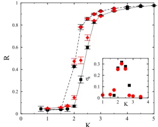
For the fully coupled network we recovered the first-order transition, known from the literature [16], as can be seen on Fig. 5. The synchronization transition occurs around K_c 2.25 for N =500 and N =1000 both and large hysteresis curves emerge as the consequence of different (fully ordered vs. randomized) initial conditions. At this resolution only weak size dependence of the transition point is observable in agreement with the results in Ref. [11]. TheσR(K) peak seems to be slightly higher in case of the larger lattice, as the inset of Fig.5shows, as opposed to the lower-dimensional cases to be discussed later.

In case of 2D lattices, with nearest-neighbor interactions and periodic boundary conditions, we found signatures of first- order phase transitions with wide hysteresis loops (see Fig.6).

The synchronization emerges very slowly by increasing K.

The finite-size scaling study showed that the order parameter curves become smoother for largerNand the transition point increases fromK100 (L=500) toK170 (L=1000).

Changinga=3 toa=1 did not cause visible differences. The time dependence of the phase synchronization order parameter can also be seen on the inset of Fig.6for a lattice of linear size

0 1 2 3 4 5

K

0 0.2 0.4 0.6 0.8 1

R

1 2 K 3 4

0 0.1 0.2 0.3 σR

FIG. 5. Hysteresis in the steady-state order parameter in fully coupled networks of sizesN=1000 (black boxes) andN=500 (red diamonds). Error bars show standard error of the mean. Inset:σR(K) peaks for the two different network sizes investigated.

L=500. There are no signs of PLs, instead theR(t) curves converge quickly to their steady-state values at allKvalues.

To investigate the hysteresis in more detail we also applied an adiabatic procedure, in which following a start from the asynchronous stateKwas increased gradually byK=0.02 steps, separated byt_K =1000 intervals, containingt_t = 900 thermalization andt_m=100 measurement regions. In this protocol the measurements were done by lineart =1 time steps and averaging was performed over 48 independent realizations of the quenched disorder. As the lower (red) curve

0 200 400 600 800

K

0 0.2 0.4 0.6 0.8 1

R

10⁰ 10² 10⁴ t 0

0.2 0.4 0.6 0.8 1

R

FIG. 6. Phase synchronization transition in the steady state in 2D networks of sizesN=500×500 (red bullets), L=1000×1000 (blue boxes) usinga=3, andN=500×500 (green stars) usinga= 1. The red lines show the results using the adiabatic protocol, started from asynchronous (bottom) or synchronous (top) states in case of N=500×500 anda=3. Error bars show standard deviation of the mean. Inset: Time dependence orR(t), in case of theN=500×500 lattice, for control parameters:K=700, 350, 200, 150, 100, 80, 60, 50 in case of synchronized initial condition (top to bottom curves) and forK=700, 100 desynchronized initial condition (top to bottom curves).

0 10 20 30 40

K

0 0.1 0.2 0.3 0.4 0.5

R

1M up 1M down 1.5M up 1.5M down 2.5M up 2.5M down US HV

FIG. 7. Steady-state order parameter for different power grid networks, usinga=3 for 1M, 1.5M, and 2.5M power grids (top to bottom curves), obtained by the adiabatic protocol. Error bars show standard errors of the mean. Pink stars correspond to the U.S. HV power grid of sizeN=4941 for comparison. We can see a vanishing synchronization and hysteresis by increasing the size.

of Fig.6forN =500×500 anda=3 shows, the synchro- nization remained very small up toK =500, in agreement with the steady-state values of the quench with desynchronized initial condition (see inset of Fig.6), but we could not reach the high branch of the solutions. When we started the adiabatic procedure from a synchronized initial condition (K=500, R=1) and decreased the coupling in the same way as in the up-sweep process, we found agreement with the high branch of solutions, obtained with the quench procedure (see top red line vs. red bullets of Fig.6).

The size of the hysteresis increased slightly by decreasing a from 3 to 1, similarly as reported in Ref. [11]. The former value was used in our subsequent, more-detailed analyses in the hope of finding critical phase transitions as the consequence of network heterogeneities.

However, we did not achieve this goal is case of the power grids we generated. Figure7shows that the transition in case of our power grids is smooth, but a critical point with PL time dependencies could not been located. Instead, fast relaxation to steady-state values was observed using the quench dynamics.

The numerical solutions exhibited large fluctuations in the time dependencies and for large Ks the solutions become unstable, even with=0.001 precision. Possible hysteresis curves now proved to be much narrower than in case of the 2D lattices. We have applied the adiabatic protocol, described in case of the 2D lattice, to provide more numerical evidence for this. Following up-sweeps, we turned back when reaching maxima at K=37 for 1M, at K=27 for 1.5M, and at K=30 for 2.5M networks. The hysteresis curves look very narrow and in case of the 1M grid a looped “hysteresis”

emerged for all random realizations of the quenched disorder.

This strange behavior remained there even for tK =2000 intervals, containing tt =1900 thermalization and tm= 100 measurement regions. We suspect this the consequence of the loopless topology of the 1M grid, different from the others. In case of the 2.5M grid we could not see hysteresis

10⁰ 10¹ 10² 10³

K

10⁻⁴ 10⁻³ 10⁻² 10⁻¹ 10⁰

σ R

500 x 500 1000 x 1000 1M a=3 2.5M a=3 US a=3

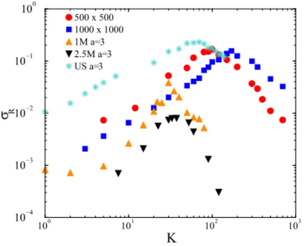
FIG. 8. Fluctuation of the steady-state order parameter for differ- ent networks witha=3. Symbols: Red bullets and blue boxes are for 2D lattices of linear sizes:L=500,1000, respectively; up triangles are for 1M grids; down triangles are for 2.5M grids; stars correspond to the U.S. HV grid.

within our error margins (standard error of the mean). So we find agreement with Ref. [11] for the Italian HV power grid, where “the transition is largely non-hysteretic, probably due to the low value of the average connectivity in such a network.”

Note that without the weight normalization (2) the transition results would have appeared at much smallerKvalues if we had used the pure admittances as weights. In case of the 1M grid we had the average,Yij =854.13/, while for the 2.5M network,Yij =763.05/. We have also considered the U.S.

HV network, in which case the results are similar to those of our synthetic networks.

Figure8shows that the steady-state order parameter fluc- tuations (σR) remained bounded and the maxima of the curves decreased when we increased the size of a given network system. Thus, we do not see signatures of a singularity, a real phase transition in the thermodynamic limit, like in case of the Kuramoto model in low (D <4) dimensions [36].

Figure8also shows the results obtained for the U.S. HV power grid, containingN =4941 nodes, usinga=3. On this small network the fluctuations are higher than those of the 2D lattices and our power grid graphs.

IV. POWER FAILURE DISTRIBUTIONS

Power failure size dependence has been studied in dif- ferent countries and heavy-tailed distributions were found, modelled by SOC models at the critical point of the their phase transitions [18,37]. Since there is no real phase transition to synchronization in the second-order Kuramoto model, we can investigate this issue in the desynchronized state only.

Following an electrical disturbance local couplings can break down and the system is indeed in the nonsynchronized state, where the effectiveKis below the transition value of the finite system. Thus measuring the behavior of the desynchronization cascade can provide information about the seriousness of the power outage. We have investigated the avalanche duration distributions by starting the system from a fully synchronous state, quenchingK to a small value and measuring the time

10³ 10⁴ 10⁵ 10⁶

t

10⁻⁵ 10⁻⁴ 10⁻³ 10⁻² 10⁻¹ 10⁰

p(t) _t^−0.83(2)

t^−1.10(2) t^−1.2(1) t^−1.75(2) t^−2.26(4) t^−3.3(9)

FIG. 9. Avalanche duration distribution for 1000×1000 lattices fora=3 at different coupling values:K=10, 5, 4, 3, 2, 1 (top to bottom solid curves). Dashed lines: PL fits for the distribution tails.

until R(tk) fell below the thresholdRT =1/√

N, related to the order parameter value of the incoherent phase. In this measurement, we averaged over10⁴runs, using independent randomω_i,0intrinsic frequencies. As we can see in Figs.9and 10, the incoherent phaseK-dependent PL decay tails emerge, similarly to GPs in other heterogeneous network models [38], very differently from an exponential decay of a random system.

Even with this large sample number the results exhibit os- cillations, especially approaching the transition region, where reachingRT requires long times. Thus we limited the range of Ks, where the decay was faster than linear. The range of the PL region can be estimated by theKvalues, where linear behavior can be fitted on thep(t) tails. This providesK <5 for the 2D lattice withN =10⁶,K <1 for the 1M power grid and K <7 for the U.S. HV network. In the latter cases the PL region is enhanced by the quenched topological heterogeneity.

In the case of a 2D lattice, without any quenched disorder, i.e., ω_i,0=0, but with an additive, annealed Gaussian frequency noise of unit variance in (1) we could not find PL tails but fast decayingp(t) distributions only.

10³ 10⁴ 10⁵

t

10⁻⁵ 10⁻³ 10⁻¹

p(t) _t^−1.17(5)

t^−1.42(2) t^−1.85(2) t^−2.50(3) t^−3.9(2)

FIG. 10. Avalanche duration distribution in the 1M power grid for a=3 and different coupling valuesK=0.7, 0.6, 0.5, 0.4, 0.2 (top to bottom solid curves). Dashed lines: PL fits for the tails.

V. FURTHER EXTENSIONS

Recently, it has been shown that a large number of decen- tralized generators, rather than a small number of large power plants, provide enhanced synchronization together with greater robustness against structural failures [39–42]. Here we studied effects of additional time-dependent stochastic noise to Eq. (1).

We added the same time-dependent random variable toω_i,0 following the probability distribution

p(ω)∼ ±e^−0.06ω, (10) which is similar to what can be read off from the MAVIR frequency fluctuation data [43].

Another attempt was the addition of a space- and time- independent, uncorrelated Gaussian noise with σ =3 vari- ance, describing a stochastic Kuramoto model. Neither of these modifications gave relevant changes in the dynamical behavior.

The annealed noise decreased the order parameter as well as its fluctuations slightly.

We have also performed preliminary calculations for bi- modal Gaussianω_i,0 distributions, modeling a coupled con- sumer or motor system [11]. Following the initial, large fluctuations the order parameter relaxes in a similar way as before but to smaller synchronization values. More detailed study of this scenario will be published later.

VI. CONCLUSIONS

We compared the phase synchronization of the second- order Kuramoto model on fully coupled, 2D lattices and real power grid networks. For this purpose we generated large synthetic networks in order to extrapolate to infinite sizes, with characteristics or real power grids. These contain millions of nodes and directed, weighted edges. Our networks exhibit hierarchical modular structure, low clustering and topological dimensions.

A real phase transition could be observed on the fully coupled graph, showing hysteresis and first-order transition.

On lower graph dimensional systems, like in the power grids or in 2D lattices smooth crossover occurs at higher global coupling values. The transition peak locations, obtained by the maximum of the fluctuations ofRare lower for the power grids:

K20–30 than in case of the 2D lattices:K100–170 of

similar sizes. The magnitudes of the fluctuations are also lower on the power grids than in the corresponding 2D lattices, albeit a decreasing tendency can be found by increasing the inertia.

The addition of a stochastic noise to Eq. (1), modeling random frequencies of distributed energy sources does not affect the synchronization too much. Even a strong Gaussian noise withσ =3 variance decreases the order parameter by 20% few percentages at most. These results point out better electrical performances in the heterogeneous networks than what simple homogeneous approximations could predict.

Scale-free tails of the avalanche duration can be observed below the transition point withK-dependent slopes. The size of this scale-free region increases with the amount of quenched disorder. For pure 2D lattices we could not found PL tails but quick decays only. This is similar to the Griffiths effects, which can occur in disordered phases of magnets in the presence of slowly decaying, rare, but large ordered regions.

However, in the lack of a real critical phase transition in the continuum limit we cannot call this a Griffiths phase. Our results are probably related to the “frustrated synchronization”

phenomena, reported recently in the case of the Kuramoto model, where modules, as rare regions, synchronize to different phases [44,45]. Understanding rare region effects in more detail in power grid models should be a subject of further studies.

We emphasize that the mechanism that would create self- organized criticality has not been assumed in our model, and still we see PL tails of event duration with similar exponents as those of the reported blackout sizes in various electrical failure data [37]. It is an open question how such additional, competing forces would modify our results.

ACKNOWLEDGMENTS

We thank Róbert Juhász and S. C. Ferreira for the useful discussions and comments. Support from the MTA-EK special grant and the Hungarian research fund OTKA (K109577) is acknowledged. The VEKOP-2.3.2-16-2016-00011 grant is supported by the European Structural and Investment Funds jointly financed by the European Commission and the Hun- garian Government. Most of the numerical work was done on NIIF supercomputers of Hungary.

[1] A. Anderssonet al., Causes of the 2003 major grid blackouts in North America and Europe, and recommended means to improve system dynamic performance,IEEE Trans. Power Syst.20,1922 (2005).

[2] J. A. Acebrón, L. L. Bonilla, C. J. Pérez Vicente, F. Ritort, and R. Spigler, The Kuramoto model: A simple paradigm for synchronization phenomena, Rev. Mod. Phys. 77, 137 (2005).

[3] A. Arenas, A. Diaz-Guilera, J. Kurths, Y. Moreno, and C. S.

Zhou, Synchronization in complex networks,Phys. Rep.469, 93(2008).

[4] G. Filatrella, A. H. Nielsen, and N. F. Pedersen, Analysis of a power grid using a Kuramoto-like model,Eur. Phys. J. B61,485 (2008).

[5] R. Carareto, M. S. Baptista, and C. Grebogi, Natural synchro- nization in power grids with anti-correlated units,Commun.

Nonlinear Sci. Numer. Simul.18,1035(2013).

[6] Y.-P. Choi, S.-Y. Ha, and S.-B. Yun, Complete synchronization of Kuramoto oscillators with finite inertia,Physica D240,32 (2011).

[7] Y.-P. Choi, Z. Li, S.-Y. Ha, X. Xue, and S.-B. Yun, Complete entrainment of Kuramoto oscillators with inertia on networks via gradient-like flow,J. Differ. Equat.257,2591(2014).

[8] F. Dorfler and F. Bullo, Synchronization and transient stability in power networks and non-uniform kuramoto oscillators,SIAM J. Control Optim.50,1616(2010).

[9] F. Dorfler and F. Bullo, Synchronization in complex networks of phase oscillators: A survey,Automatica50,1539(2014).

[10] M. Frasca, L. Fortuna, A. S. Fiore, and V. Latora, Analysis of the Italian power grid based on kuramoto-like model, inProceedings of the 5th International Conference on Physics and Control (PhysCon 2011)(IPACS Electronic library, Leon, Spain, 2011).

[11] S. Olmi, A. Navas, S. Boccaletti, and A. Torcini, Hysteretic transitions in the Kuramoto model with inertia, Phys. Rev. E 90,042905(2014).

[12] R. S. Pinto and A. Saa, Synchrony-optimized networks of Kuramoto oscillators with inertia,Physica A463,77(2016).

[13] K. Schmietendorf, J. Peinke, R. Friedrich, and O. Kamps, Self-organized synchronization and voltage stability in networks of synchronous machines,Eur. Phys. J. Spec. Top.223,2577 (2014).

[14] J. M. Grzybowski, E. E. Macau, and T. Yoneyama, On synchro- nization in power grids modelled as networks of second-order Kuramoto oscillators,Chaos26,113113(2016).

[15] Y. Kuramoto,Chemical Oscillations, Waves, and Turbulence (Springer, Berlin, 1984).

[16] H.-A. Tanaka, A. J. Lichtenberg, and S. Oishi, First Order Phase Transition Resulting from Finite Inertia in Coupled Oscillator Systems,Phys. Rev. Lett.78,2104(1997).

[17] G. Ódor, Nonequilibrium Lattice Systems (World Scientific, Singapore, 2008).

[18] B. A. Carreras, D. E. Newman, I. Dobson, and A. B. Poole, Evidence for self-organized criticality in a time series of electric power system blackouts,IEEE Trans. Circuit Syst. I: Regular Papers51,1733(2004).

[19] P. Bak, C. Tang, and K. Wiesenfeld, Self-organized criticality, Phys. Rev. A38,364(1988).

[20] T. Vojta, Rare region effects at classical, quantum and nonequi- librium phase transitions, J. Physics A: Math. Gen.39,R143 (2006).

[21] P. V. Martin, J. A. Bonachela, and M. A. Muñoz, Quenched disorder forbids discontinuous transitions in nonequilibrium low-dimensional systems,Phys. Rev. E89,012145(2014).

[22] R. B. Griffiths, Nonanalytic Behavior above the Critical Point in a Random Ising Ferromagnet,Phys. Rev. Lett.23,17(1969).

[23] G. Ódor, Slow, bursty dynamics as a consequence of quenched network topologies,Phys. Rev. E89,042102(2014).

[24] G. A. Pagani,From the Grid to the Smart Grid, Topologically, PhD dissertation (Rijskuniversiteit Groningen, 2014).

[25] T. Gómez, C. Mateo, Á. Sánchez, P. Frias, and R. Cossent, Reference network models: A computational tool for planning and designing large-scale smart electricity distribution grids, in HPC in Power and Energy Systems, edited by S. K. Khaitan and A. Gupta (Springer Science & Business Media, 2013), 247–279.

[26] Z. Whang and R. J. Thomas, Random topology power grid modeling and automated simulation platform, CERTS Rev.5–6, (2014).

[27] S. Pahwa, C. Scoglio, and A. Scala, Abruptness of cascade failures in power grids,Sci. Rep.4,3694(2014).

[28] S. Ma, Y. Yu, and L. Zhao, Dual-stage constructed random graph algorithm to generate random graphs featuring the same

topological characteristics with power grids,J. Mod. Power Syst.

Clean Energy5,683(2017).

[29] D. J. Watts and S. H. Strogatz, Collective dynamics of “small- world” networks,Nature393,440(1998).

[30] M. E. Newman, C. Moore, and D. J. Watts, Mean-Field Solution of the Small-World Network Model,Phys. Rev. Lett.84,3201 (2000).

[31] US power grid, http://konect.uni-koblenz.de/networks/opsahl- powergrid

[32] Z. Wang, R. J. Thomas, and A. Scaglione, Generating random topology power grids, inProceedings of the 41st Annual Hawaii International Conference on System Sciences (HICSS 2008) (IEEE, Piscataway, NJ, 2008).

[33] P. Schulz, J. Heitzig, and J. Kurths, A random growth model for power grids and other spatially embedded infrastructure networks,Eur. Phys. J. Spec. Top.223,2593(2014).

[34] A. Patania, J. Young, S. Lumbreras, M. G. Pereda, I. Bertazzi, D.

Citron, and M. Haraguchi, Complex Systems Techniques applied to Power Transmission Expansion Planning. Part I : Generating Random Networks that are Consistent with Power Transmission, This working paper has been produced as a result of the work carried out at the 2015 Complex Systems Summer School at the Santa Fe Institute.

[35] Numerical Recipes,http://numerical.recipes.

[36] H. Hong, H. Park, and M. Y. Choi, Collective Synchronization in Spatially Extended Systems of Coupled Oscillators with Random Frequencies,Phys. Rev. E72,036217(2005).

[37] I. Dobson, B. A. Carreras, V. E. Lynch, and D. E. Newman, Complex systems analysis of series of blackouts: Cascading failure, critical points and self-organization,Chaos17,026103 (2007).

[38] G. Ódor, Critical dynamics on a large human Open Connectome network,Phys. Rev. E94,062411(2016).

[39] M. Rohden, A. Sorge, M. Timme, and D. Witthaut, Self- Organized Synchronization in Decentralized Power Grids,Phys.

Rev. Lett.109,064101(2012).

[40] T. D. Witthaut and M. Timme, Braess’s paradox in oscillator networks, desynchronization and power outage,New J. Phys.

14,083036(2012).

[41] M. Rohden, A. Sorge, D. Witthaut, and M. Timme, Impact of network topology on synchrony of oscillatory power grids, Chaos24,013123(2014).

[42] M. J. Lee and B. J. Kim, Spatial uniformity in the power grid system,Phys. Rev. E95,042316(2017).

[43] Data of the Hungarian electrical system,https://www.mavir.hu/

documents/10258/45985073/MAVIR_VER_2017_web.pdf, (MAVIR 2016).

[44] P. Villegas, P. Moretti, and M. A. Muñoz, Frustrated hierarchical synchronization and emergent complexity in the human connec- tome network,Sci. Rep.4,5990(2014).

[45] A. P. Millán, J. J. Torres, and G. Bianconi, Complex network geometry and frustrated synchronization, Sci. Rep. 8, 9910 (2018).