MohammadReza Saadat, Benedek Nagy
Department of Mathematics, Faculty of Arts and Sciences, Eastern Mediterranean University, 99450 Famagusta, North Cyprus, Mersin-10, Turkey
{mohammed.saadet | benedek.nagy}@emu.edu.tr
Abstract: Cellular automata are parallel computing devices working on a discrete time- scale. In the paper, each cell of the triangular grid has a state from the binary set (i.e., we have a binary pattern, an image, on the grid), and the state in the next time instant depends only on the actual state of the cell itself and the states of its side-neighbor cells. We illustrate their use in image synthesis, e.g., generating snowflakes, and in image analysis: some of our automata are connected to image processing operations, e.g., dilation and erosion.
Computation of Hausdorff distance of two binary images on the triangular grid is also presented. In image processing, and especially in mathematical morphology, operations are local operations, and thus, cellular automata are apt to use. On the other side, the triangular grid is not a point lattice, thus the definition of translation based image operations is not always straightforward.
Keywords: parallel computing; cellular automaton; non-traditional grids; binary image processing; game of life; dilation; erosion; closing; opening; Hausdorff distance
1 Introduction
Cellular automata are widely used classical parallel computing models formulated by von Neumann, Ulam and Codd in the 1940’s. These automata work on discrete grids, each cell has a state from a finite set and they are able, e.g., to do “self- reproduction”. 2D models are widespread [7, 10, 24, 27]; “Game of Life” is one of the most popular cellular automata, it was introduced in 1970 by Conway [8, 9, 10, 23]. It is designed on a square grid where each cell has only 2 states: dead or alive.
Many life-like automata have been studied since then (see, e.g, [5]). One of the most important properties of the cellular automata is the type of the grid. There are various two dimensional infinite grids: square, triangular, pentagonal and hexagonal grids. Digital image processing and mathematical morphology use discrete images represented on a grid. There are various algorithms which are based on the value of the cell and on the values of its neighbors. This fact gives us the possibility to
establish relations between specific cellular automata and morphological operations.
Image processing and image analysis are important parts of artificial and computational intelligence. The most used digital space is the square grid, it is used most frequently in applications as well. There are two other regular tessellations of the plane, the hexagonal and the triangular grids; they are also in a duality relation in terms of planar graphs. Because of some better properties some of the image processing algorithms are also developed for these grids [15, 18, 21, 13]. However, the triangular grid is not a point lattice, thus translation based local operations cannot be defined in a straightforward way. This is an important difference from the square and hexagonal lattices. In mathematical morphology, dilation and erosion are based on local translations, various approaches to extend their definitions to the triangular grid was shown recently in [1]. This paper is also motivated by the reason of lack of morphological operations described and analysed on the triangular grid.
In various image processing applications parallel and distributed algorithms become important and popular, we will present parallel algorithms (cellular automata) for morphological operations.
In this paper, we are going to study cellular automata on the triangular grid giving some general characteristics. Some models can be connected to image processing techniques, especially parallel algorithms to dilation and erosion. Cellular automata were already introduced on the triangular grid [4], but with a larger neighborhood (for a Moore-type of neighbourhood having 12 neighbors). Here, in this paper, the smallest natural neighborhood (with 3 neighbors) is considered, that is analogous to the von Neumann neighbourhood used in the square grid.
2 Preliminaries
2.1 Cellular Automaton
A cellular automaton consists of a regular grid of cells with finite number of dimensions. Each cell has a finite number of states, such as “on” and “off” (In case of 2 states, it is called binary). For each cell, there is a set of cells called its neighbors. An initial state (time t = 0) is where each cell has one specified state (e.g., “on” or “off”). A new generation (t + 1) is created according to some fixed rules that specify the new state of each cell based on its current state and its neighbors’ states. The rules are the same for each cell and do not change. They are simultaneously applied to the whole grid. In the next subsection we recall a specific binary model.
initial state, requiring no further input, thus it is a zero-player game. To “play” this game one creates an initial pattern and observes how it generates the next ones. It runs in a space of unlimited two-dimensional square grid. Each cell has two possible states, dead or alive, and interacts with its eight neighbors that are adjacent diagonally, vertically, or horizontally. This Moore neighborhood, also called chessboard neighborhood in image processing, is defined as
𝑁(𝑥, 𝑦) = {(𝑥′, 𝑦′)|𝑥′∈ {𝑥 − 1, 𝑥, 𝑥 + 1}, 𝑦′∈ {𝑦 − 1, 𝑦, 𝑦 + 1}}\{(𝑥, 𝑦)}
The game has simple rules which are as follow:
Birth: a dead cell at time t with exactly 3 living neighbors will be alive at time t + 1.
Death: a living cell at time t with less than 2 or more than 3 living neighbors will die at time t + 1.
The initial pattern is the system’s seed. Each generation is a function of the previous one. The generation t + 1 is created by applying the game’s rules simultaneously to each cell in the generation t. The rules are applied repetitively to create the next generations.
2.3 Triangular Grid
The Triangular Grid is also called isometric grid; it is a grid generated by tiling the plane regularly with equilateral triangles. Various coordinate systems can be used for this grid. Here we use the one which was described in [16, 17, 15]. Each cell has 3 coordinates, i, j and k where
i , j , k
andi j k 0 , 1
. See also Figure 1(a). There are 2 types of cell: type ”E“, even cells, where the sum of coordinates equals to 0 and type ”O“, odd cells, where the sum of coordinates equals to 1.Closest neighbors, also called side-neighbors are used throughout this paper. Two cells are neighbors if exactly one of their coordinates differs, and this difference is
±1. Consequently, each cell has 3 neighbors, the cells with which it shares a side.
Even cells have odd neighbors and vice versa. Example of neighbors can also be seen in Figure 1(b) and (c), respectively.
Figure 1
(a) Triangular grid. (b) A cell type “E” and (c) a cell type “O” with their neighbors
3 Definitions
Each cell has 2 possible states: dead or alive, they are represented by colors: black cells are alive, white cells are dead. A pattern is a set of living cells on the triangular grid. A starting state is just a finite pattern in the triangular grid.
The next definitions are somewhat analogous to the embedding hexagon of [20].
Definition 1. The Bounding Hexagon of a pattern is the smallest hexagon on the triangular grid which contains the pattern properly inside of itself. We use notation B for the Bounding Hexagon.
Let 𝐻1= {(𝑥, 𝑦, 𝑧)|𝑥𝑚𝑖𝑛− 1 ≤ 𝑥 ≤ 𝑥𝑚𝑎𝑥+ 1, 𝑦𝑚𝑖𝑛− 1 ≤ 𝑦 ≤ 𝑦𝑚𝑎𝑥+ 1, 𝑧𝑚𝑖𝑛− 1 ≤ 𝑧 ≤ 𝑧𝑚𝑎𝑥+ 1 }, then 𝐵 = {(𝑥, 𝑦, 𝑧) ∈ 𝐻1|𝑥 = 𝑥𝑚𝑖𝑛− 1 or 𝑥 = 𝑥𝑚𝑎𝑥+ 1 or 𝑦 = 𝑦𝑚𝑖𝑛− 1 or
𝑦 = 𝑦𝑚𝑎𝑥+ 1 or 𝑧 = 𝑧𝑚𝑖𝑛− 1 or 𝑧 = 𝑧𝑚𝑎𝑥+ 1 }.
Definition 2. Outer Hexagon is the smallest Hexagon on the triangular grid which contains the bounding hexagon properly inside of itself. We use notation O for the Outer Hexagon.
Let 𝐻2= {(𝑥, 𝑦, 𝑧)|𝑥𝑚𝑖𝑛− 2 ≤ 𝑥 ≤ 𝑥𝑚𝑎𝑥+ 2, 𝑦𝑚𝑖𝑛− 2 ≤ 𝑦 ≤ 𝑦𝑚𝑎𝑥+ 2, 𝑧𝑚𝑖𝑛− 2 ≤ 𝑧 ≤ 𝑧𝑚𝑎𝑥+ 2 }, then 𝑂 = {(𝑥, 𝑦, 𝑧) ∈ 𝐻1|𝑥 = 𝑥𝑚𝑖𝑛− 2 or 𝑥 = 𝑥𝑚𝑎𝑥+ 2 or 𝑦 = 𝑦𝑚𝑖𝑛− 2 or
𝑦 = 𝑦𝑚𝑎𝑥+ 2 or 𝑧 = 𝑧𝑚𝑖𝑛− 2 or 𝑧 = 𝑧𝑚𝑎𝑥+ 2 }.
See Figure 2, for examples.
Figure 2
A sample pattern (black), its bounding hexagon (blue) and its outer hexagon (green) Definition 3. A BS-Automaton on the triangular grid consists of a starting state and its rule R that is a combination of 2 sets. The first set is called “Birth” (shortly “B”) which shows the number of living cells needed in the neighborhood of a dead cell to make it alive. The second set is called “Survival” or “Stay alive” (“S”) which shows the number of living cells needed in the neighborhood of a living cell to keep it alive.
𝑅 ∈ {B𝑥S𝑦|𝑥, 𝑦 ∈ {0,1,2,3}∗ are strings containing each of the numbers at most once}.
Since we have 3 neighbors, it is clear that B and S are subsets of M = {0,1,2,3}, and the above notation is used where string x contains the elements of B and y contains the elements of S. Both for B and S there are 24 possible sets, thus the total number of possible rules of BS-automata is 256. In the next section we show some of their properties.
4 Results
We start the section with some general observations.
Theorem 1. Any BS-automaton with rule R: 0 ∈ 𝐵 and 3 ∉ 𝑆 leads to alternating states such that every second state consists of infinitely many living cells.
Proof: Based on the definition, the starting state is a set of finitely many living cells.
If we consider the Outer Hexagon of the pattern, every cell outside of this hexagon is dead and has only dead neighbors. Since 0 is included in B, in the next step all these cells become alive, thus we have infinitely many living cells which have 3 living neighbors and only finitely many without 3 living neighbors. For the next generation, since 3 is not included in the set S, all these cells would die, and then, we have finitely many living cells and infinitely many dead cells. This property of
the pattern is repeated by period 2. □
Further, we assume that our automaton is not of the previously described “flashing”
type, and we deal with BS-automata with the condition 0 ∉ 𝐵.
Theorem 2. Any BS-automaton with rule R with 1 ∈ B leads to an unbounded growth (concerning the size of the pattern).
Proof. If we consider the Bounding Hexagon of the pattern, there would be 1 or more boundary cells which share an edge or a vertex with the Bounding Hexagon.
If at least 1 boundary cell shares an edge with the Bounding Hexagon, then at the next step, since 1 ∈ 𝐵, its neighbor cell in the Bounding Hexagon becomes alive.
This means that the new Bounding Hexagon is bigger than the previous one in this direction.
If none of the boundary cells share an edge with the Bounding Hexagon, then at the next step, at least one cell becomes alive such that it shares an edge with the Bounding Hexagon. Thus, even the new Bounding Hexagon would be the same size, at the next step, as we have shown in the previous part of the proof, the new Bounding Hexagon will be bigger.
The unlimited increase of the Bounding Hexagon shows the unbounded growth of
the automaton. □
4.1 Case Studies with Growing Patterns
After some general results we are going to study some specific BS-automata.
Case B1S0123. In this automaton since S equals to M, any living cells live forever.
By Theorem 2, there is no stable or periodic pattern. It usually makes the shape of snowflakes. It will never stop and it goes to infinity. Regardless of the type(s) of the starting cell(s) (“E” or “O”), it generates similar patterns. Figure 3 presents sample 1 where the starting state is a single cell of type “O”. It also presents a real snowflake in the ending of the second line for the comparison. In Sample 2 the starting state is consisting of 2 separate cells with different types, as one can see on Figure 4, the growth of the pattern is very similar to the previous example. This automaton can be used for image synthesis.
Figure 3
Automaton B1S0123, Sample 1, and a real snowflake1comparing to generation 20
1 SnowCrystals.com. Web. 1 Jan. 2017. <http://www.snowcrystals.com/>
Figure 4
Automaton B1S0123, Sample 2
Case B1S123. Since the birth condition is 1, there is no stable pattern. Also there is no periodic pattern and it goes on to infinity. It generates inherently different patterns depending on the fact that the staring state includes only one type of cells or both types. If the starting state has only one type of cells, then after each step we have only one type of cells. In sample 3 the starting state consists of a single cell of type “O”. It starts with type “O” and after that only type “E” cells are alive, and this property is repeated with period 2. See Figure 5. In the next sample the starting state is consisting of 2 adjacent cells with different types. Surprisingly, we got back very similar snowflake as we have seen in case of automaton B1S0123. Actually the two automata generate the same sequence of patterns from this start state. See Figure 6.
Figure 5
Automaton B1S123, Sample 3
Figure 6
Automaton B1S123, Sample 4
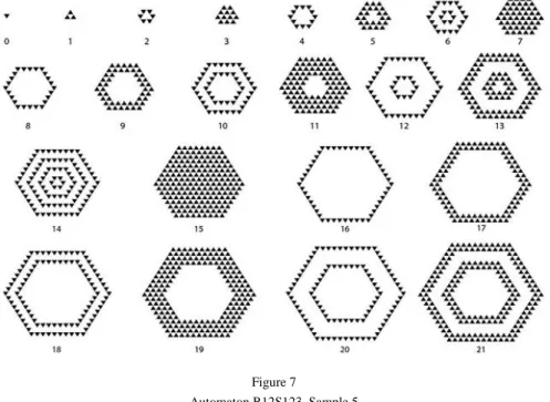
Case B12S123. Since 1 is included in the set of birth conditions, there is no stable and no periodic pattern; it grows to infinity. If we start with one type of cells the method generates pattern similar to water’s wave. In Sample 5, the starting state consists of a single cell of type “O”. In each step we only have cells of one type.
See Figure 7. This method has completely different behavior when we have both types of cells in the starting state. In such cases it fills the whole space easily and also, sometimes we may have finitely many holes. In sample 6 the starting state consists of 3 separate cells. There are 2 cells of type “O” and 1 cell of type “E”.
Figure 8 shows this example.
4.2 BS-Automata related to Image Processing
Case B2S0123. In this case any starting pattern will be transformed to a stable pattern soon and there is no infinite growth. Also since S equals to M, any living cells live forever. This automaton is a good tool for filling small spaces between cells. Sample 7 is transformed to a stable pattern in one generation, as it is shown in Figure 9 (2 left images).
Figure 7
Automaton B12S123, Sample 5
Figure 8
Automaton B12S123, Sample 6
Figure 9
B2S0123, Sample 7 (2 left images); Sample 8 (middle) and Sample 10 (right) are stable In Sample 8, we have 2 lines with distance 1. This is a stable pattern and the automaton does not change the generation 0 (see Figure 9 (middle)). Next we add one single living cell to the left end. The automaton starts to fill the empty spaces between the 2 lines step by step and then arrives to a stable pattern on generation 11, as Figure 10 shows. However, it cannot be used to fill more than 1 cell width holes (Sample 10, in Figure 9).
Figure 10
Automaton B2S0123, Sample 9
This automaton can be used for image recovery. In Sample 11 we have a set of living cells which should represent letter “Z”. However, some of the living cells were deleted. The shape of Z is established after some generations. However, this automaton cannot filter out usual salt and pepper noises; see Sample 12 (Figure 12).
Figure 11
Automaton B2S0123, Sample 11, reconstruction of the character “Z”
Figure 12
Automaton B2S0123, Sample 12
It could repair some patterns but couldn’t remove the usual noises.
Case B2S123. This case is similar to the case B2S0123 but since 0 is not included in S, every living cell needs at least one living cell in its neighborhood to stay alive.
With this automaton we have stable shapes and also periodic shapes (see Figure 13, Sample 13, left) but no infinite growth. This automaton gives us an important ability of Noise Filtering. Sample 14 is supposed to represent the word “Hi”. Run of the automaton results to a stable pattern in 3 generations. (See Figure 13, Sample 14, middle.) This method still cannot filter inner noises (salt noise), see Figure 13, Sample 12, right.
Figure 13
Automaton B2S123, Sample 13, an oscillator with period 2 (left), noise filtering on word “Hi”, Sample 14 (middle) and Sample 12, (right)
Case B23S123. With this automaton we may have stable shapes and periodic shapes but not infinite growth. The automaton can be used to repair the shapes, to remove the outer noises (pepper) and to fill the inner noises (salt) at the same time, see Figure 14, left. Usage of this automaton also has some disadvantages. It will completely delete Sample 15 in 5 generations as it is shown in Figure 14 (right).
Figure 14
Automaton B23S123, Sample 12 (left), Sample 15 (right)
By the next examples we take the next step to the direction of image processing applications.
4.3 Pattern Recovery by Combining BS-Automata
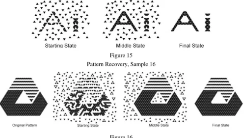
Using a combination of two or more automata can help to recover the patterns and to filter the noises. One solution is to apply automaton B2S0123 first, then automaton B23S123 to the stable state obtained by automaton B2S0123 (we may call it middle state of the process). We used this method for Sample 16, see Figure 15. We have also tested the method on the Logo of our university (Eastern Mediterranean University, see Figure 16, left). Some noises are applied (2nd picture of Figure 16) on the original pattern and we used this image as the starting state.
Figure 16 shows not only the original pattern and the starting state, but the middle state and final (stable) state as well. The finally obtained stable state is almost the same as the original pattern: the difference contains only 2 cells.
Figure 15 Pattern Recovery, Sample 16
Figure 16
Pattern Recovery, Sample 17, Logo of the “Eastern Mediterranean University”
5 Morphologic Operations
Definition 4. The dilation of a pattern A on the triangular grid is a pattern D(A) such that:
𝐷(𝐴) = {𝑞|𝑞 ∈ 𝐴 or at least one of the neighbors of 𝑞 is an element of 𝐴}.
Definition 5. The erosion of a pattern A on the triangular grid is a pattern E(A) such that:
𝐸(𝐴) = {𝑞|𝑞 ∈ 𝐴 and all the neighbors of 𝑞 are elements of 𝐴}.
Note that the dilation and erosion above are done by the neighborhood used in this paper. In paper [1] similar operations are defined in a more general manner, instead of a fixed neighbourhood, various structural elements were used with various constraints. Allowing only vectors that translate the grid to itself, the strict approach is defined. In the weak approach each grid point can be used for translation.
However, to describe our neighbourhood relation one may also need vectors with value (-1) as the sum of its coordinates, e.g., (-1,0,0). In the strong variants any three dimensional vectors are allowed to use, but only those triplets can be displayed which have 0 or +1 sum. Our special definition here is compatible only with this most general variant of operations of the mentioned paper having the following7- element set as structural element including the following 6+1 vectors {(0,0,1),(0,1,0),(1,0,0),(0,0,-1),(0,-1,0),(-1,0,0),(0,0,0)}.
By checking the definition of our automata one can establish the following:
Theorem 3. The automaton B123S0123 is equivalent to dilation.
Proof. Assume that 𝑞 ∈ 𝐷(𝐴), then either 𝑞 ∈ 𝐴 or there is a 𝑞′∈ 𝐴 such that 𝑞 and 𝑞′ are neighbors. Let us run B123S0123 on A. Clearly if 𝑞 ∈ 𝐴 then it is element of the resulted image because S0123, i.e., each pixel of A survives. If 𝑞 ∉ 𝐴 but there is a 𝑞′∈ 𝐴 such that 𝑞 and 𝑞′ are neighbors, then 𝑞 is also element of the resulted image because of B123.
Now, let us assume that 𝑞 is an element of the resulted image of running B123S0123 on 𝐴, then either because of S0123, 𝑞 ∈ 𝐴 or because of B123, there is a 𝑞′∈ 𝐴 such that 𝑞 and 𝑞′ are neighbors which in both cases imply that 𝑞 ∈ 𝐷(𝐴).
□ Theorem 4. The automaton BS3 is equivalent to erosion.
Proof. Assume that 𝑞 ∈ 𝐸(𝐴), then 𝑞 ∈ 𝐴 and also all of its neighbors are element of 𝐴. Let us run BS3 on A. Clearly if q is element of the resulted image, then because of S3, q and all of its neighbors are elements of A which means 𝑞 ∈ 𝐸(𝐴).
□ Definition 6. The opening of a pattern A on the triangular grid is the pattern D(E(A)).
Figure 17
A pattern and its various morphologic transformations
Definition 7. The closing of a pattern A on the triangular grid is the pattern E(D(A)).
Similarly to the already shown combinations of BS-automata, one can apply 1 step with B123S0123 and then 1 step with BS3 to obtain the closing of the original pattern. Using these automata in the opposite order, the opening of the original image is obtained. See also Figure 17. Based on the distance of pixels measured by the length of the shortest path(s) connecting them through neighbor pixels (for more details we refer to, e.g., [16, 17, 15, 13]) we can also introduce the distance of patterns (see, e.g., [14]). This, so-called Hausdorff-distance, is used to measure, e.g., image similarities.
Definition 8. The Hausdorff-distance of two patterns A and B is defined as 𝑑(𝐴, 𝐵) = max {max
𝑝∈𝐴 min
𝑞∈𝐵𝑑(𝑝, 𝑞) , max
𝑝∈𝐵 min
𝑞∈𝐴𝑑(𝑝, 𝑞)}.
It is known that the Hausdorff-distance can be computed by dilations: By counting the minimum number of dilations that one needs to make on A to get a pattern Dn(A) such that Dn(A) B, and vice-versa, the minimal m such that Dm(B) A, and finally taking the maximum of n and m gives exactly the value of d(A,B) (see, e.g, [14]).
Figure 18 shows an example. Obviously, the iterated dilations can be done by applying B123S0123 on both images.
Figure 18
Patterns A and B (up), and their iterated dilation with 2 and 3 steps, respectively, resulting an image containing the other one, this yields to d(A,B) = 3
6 Literature Review
In this section the relation of our results and some results from the literature is shown. First we consider cellular automata related literature, then, we discuss also image processing algorithms, concentrating on those models that are defined on the triangular grid.
Cellular automata have already been defined and used in various grids. As we have already mentioned, in [4], Bays described cellular automata on the regular triangular grid, but based on 12 neighbors of the cells. In [4] stable patterns and gun like shapes were analysed in connection to Conway’s Game of Life. Bays has also extended some notions on the pentagonal and hexagonal grids in [6]. In [11] it is analysed how messages can be transported in various grids based on a cellular automata approach. A new family of hexavalent networks stabilizing the symmetry axes,
sequences. In [25] cellular automata on the regular triangular and hexagonal grids are used for path planning of robots based on artificial intelligence algorithms. In [3] cellular automata with memory are used to provide a reversible model on the triangular grid which may be helpful in bio- and physics related modelling and applications. In [26], triangles on specific topologically surfaces defined the grid of the cellular automata. In [29] the developments of the patterns are studied on any triangulated surface. Only grids with finitely many triangles are considered.
Although the used grid is usually irregular triangular mesh, each triangle (except those that are on the boundary of the surface) has three neighbors, thus the rules of the automata are somewhat similar to those that we will define. However, the behaviour of the automata is different. In irregular meshes, no general coordinate system, no lanes, even and odd pixels are defined. Although cellular automata only on the square grid were used in [22], we should recall that, the authors used cellular automata for image processing applications such as noise removal and edge detecting. In this way, our paper can also be seen as a kind of extension of some of the results of [22] to the triangular grid. However we have used only deterministic cellular automata, while in [22] non deterministic model is considered for noise removal.
Morphological operations dilation and erosion are considered for the triangular grid in a more general and mathematical approach in [1, 2]. Our aim here was to show how cellular automata can be applied in mathematical morphology and other related image processing tasks on the triangular grid. We have shown also opening and closing and other image processing operations. About filtering operations, we briefly mention the median filtering. For binary images, in fact, this filtering assigns for each pixel the color of the majority of the pixels in its neighborhood. Notice that it works nicely on the square grid with both the usual used city block (von Neumann) and chessboard (Moore) neighborhood, since a pixel with their neighbors consist of 5 and 9 pixels, respectively [12]. However, this method does not work on the triangular grid using the closest neighbourhood, since a pixel with its 3 neighbors may have no majority color. On the triangular grid, median filter based on the 12 neighbors of the pixels can be defined, see, e.g., [28]. Considering the triangular grid with the closest neighbors, we may modify a little bit the original concept of the median filter. If we keep a pixel 0 only if the average of the value of the 4 pixel (the pixel and its 3 neighbors) is less than 0.5, and set it to 1 if this value is at least 0.5, we got a somewhat similar filter. In fact, a pixel is set to value 1, if at least 2 of the 4 pixels had value 1. Figure 19 shows how this filtering method can recover a noisy pattern (left). Applying it 35 times, the pattern is recovered (right) with a relatively small pixel error (18 pixels). By comparing this result to Fig. 16, we may see that our method with cellular automata shows a better performance (2 pixel error). Actually, our filtering method is based on morphological type of operations, as we have discussed.
Figure 19
Pattern Recovery by a median like filter (the right figure, a stable pattern, is obtained after 35 steps) Conclusions
In this paper various cellular automata are shown, some of them imply infinite growth of patterns; some of them reach a stable pattern or lead to a periodic behavior. Some of them are used to do some pattern recovery (step by step) filling concavities and holes; others can be used to remove noise. We have also shown how specific models can do dilation and erosion. These models are entirely parallel methods of computing. Based on them, further morphologic operations, the opening and closing were also computed. Further, by an iterative application of the automata for dilation, the Hausdorff distance of patterns on the triangular grid is computed.
Parallel computing becomes very popular in practice, since more and more hardware devices support it, thus these approaches are valid alternatives to the traditional sequential computations (which are still frequently used on images).
In order to create the figures and find the properties of each case considered we have designed a Windows application using Microsoft Visual Studio 2015 platform.
This software was used for the simulations presented.
References
[1] Abdalla M., Nagy B. (2017) Concepts of Binary Morphological Operations Dilation and Erosion on the Triangular Grid. In: Barneva R., Brimkov V., Tavares J. (eds) Computational Modeling of Objects Presented in Images.
Fundamentals, Methods, and Applications. CompIMAGE 2016, Lecture Notes in Computer Science, Vol. 10149, Springer, Cham, 89-104
[2] Abdalla, M., Nagy, B. (2018) Dilation and Erosion on the Triangular Tessellation: an Independent Approach. IEEE Access, 6, 23108-23119 [3] Alonso-Sanz, R. (2007) A Structurally Dynamic Cellular Automaton with
Memory in the Triangular Tessellation. Complex Systems, 17, 1-15 [4] Bays, C. (1994) Cellular Automata in the Triangular Tessellation. Complex
Systems, 8(2), 127-150
Tessellations. In: Meyers R. (eds) Computational Complexity. Springer, New York, pp. 434-442
[7] Delorme, M., Mazoyer, J., Cellular Automata: A Parallel Model, Springer, 1998
[8] Ewert, W., Dembski, W., Marks, R. J. (2015) Algorithmic specified complexity in the Game of Life. Systems, Man, and Cybernetics: Systems, IEEE Tr., 45(4), 584-594
[9] Gardner, M. (1970) Mathematical Games: The Fantastic Combinations of John Conway’s New Solitaire Game “Life”. Scientific American, 223(4), 120-123
[10] Herendi, T., Nagy, B.: Parallel Approach of Algorithms, Typotex, Budapest, 2014
[11] Hoffmann, R., Désérable, D. (2015) Routing by Cellular Automata Agents in the Triangular Lattice. In Robots and Lattice Automata (pp. 117-147) Springer, Cham
[12] Huang, T., Yang, G. J. T. G. Y., Tang, G. (1979) A Fast Two-Dimensional Median Filtering Algorithm. IEEE Transactions on Acoustics, Speech, and Signal Processing, 27(1) 13-18
[13] Kardos, P., Palágyi, K. (2017) On Topology Preservation of Mixed Operators in Triangular, Square, and Hexagonal Grids. Discrete Applied Mathematics, 216 (2017) 441-448
[14] Klette, R., Rosenfeld, A.: Digital Geometry: Geometric Methods for Digital Picture Analysis. Morgan Kaufmann, 2004
[15] Nagy, B (2004) Characterization of Digital Circles in Triangular Grid.
Pattern Recognition Letters, 25 (2004) 1231-1242
[16] Nagy, B. (2001) Finding Shortest Path with Neighborhood Sequences in Triangular Grids, ISPA 2001, 2nd IEEE Int. Symp. Image and Signal Processing and Analysis, 55-60
[17] Nagy, B. (2002) Metrics based on Neighbourhood Sequences in Triangular Grids, Pure Mathematics and Applications - PU.M.A. 13, 259-274
[18] Nagy, B. (2007) Distances with Neighbourhood Sequences in Cubic and Triangular Grids. Pattern Recognition Letters, 28, 99-109
[19] Nagy, B. (2017) Application of Neighborhood Sequences in Communication of Hexagonal Networks, Discrete Applied Mathematics 216, 424-440
[20] Nagy, B., Barczi, K. (2013) Isoperimetrically Optimal Polygons in the Triangular Grid with Jordan-Type Neighbourhood on the Boundary.
International Journal of Computer Mathematics, 90(8) 1629-1652
[21] Nagy, B., Lukic, T. (2016) Dense Projection Tomography on the Triangular Tiling. Fundam. Inform. 145, 125-141
[22] Popovici, A., Popovici, D. (2002) Cellular Automata in Image Processing. In Proceedings of the Fifteenth International Symposium on Mathematical Theory of Networks and Systems, D. S. Gilliam and J. Rosenthal, Eds., electronic proceedings, 6 pages
[23] Rendell, P. (2002) Turing Universality of the Game of Life. In collision- based computing (pp. 513-539) Springer, London
[24] Rozenberg, G., Bäck, T., Kok, J.N. (eds.) Handbook of Natural Computing.
Springer 2012
[25] Tariq, J., Kumaravel, A. (2016) Construction of Cellular Automata over Hexagonal and Triangular Tessellations for Path Planning of Multi-Robots.
2016 IEEE International Conference on Computational Intelligence and Computing Research (ICCIC) 6 pages, IEEE (doi: 10.1109/ICCIC.2016.
7919686)
[26] Warne, D. J., Hayward, R. F. (2015) The Dynamics of Cellular Automata on 2-Manifolds is Affected by Topology. J. Cellular Automata, 10(5-6) 319-339 [27] Wolfram, S.: A New Kind of Science. Champaign, IL: Wolfram Media, 2002 [28] Yagou, H., Belyaev, A., Wei, D. (2002) Mesh Median Filter for Smoothing 3-D Polygonal Surfaces. In Cyber Worlds, 2002. Proceedings. First International Symposium on. IEEE. pp. 488-495
[29] Zawidzki, M. (2011) Application of Semitotalistic 2D Cellular Automata on a Triangulated 3D Surface. International Journal of Design & Nature and Ecodynamics, 6(1) 34-51