Experiments on the distance of two-dimensional samples

Experiments on the distance of two-dimensional samples

Csaba Noszály

University of Debrecen, Faculty of Informatics, Debrecen, Hungary e-mail: noszaly.csaba@inf.unideb.hu

Dedicated to Mátyás Arató on his eightieth birthday

Abstract

The distance of two-dimensional samples is studied. The distance is based on the optimal matching method. Simulation results are obtained when the samples are drawn from normal and uniform distributions.

Keywords:Optimal matching, simulation, Gaussian distribution, goodness of fit, general extreme value distribution.

MSC: 62E17, 62H10

1. Introduction

A well-known result in optimal matchings is the following (see Ajtai-Komlós-Tus- nády [1]). Assume that both X1, . . . , Xn and Y1, . . . , Yn are independent identi- cally distributed (i.i.d.) random variables with uniform distribution on the two- dimensional unit square. Let X1, . . . , Xn and Y1, . . . , Yn be independent of each other. Let

tn= min

π

Xn i=1

||X_π(i)−Yi||, (1.1) where the minimum is taken over all permutationsπof the firstnpositive integers.

Then

C1(nlogn)^1/2< tn< C2(nlogn)^1/2 (1.2) with probability1−o(1)(Theorem in [1]). tn is the so-called transportation cost.

Talagrand in [6] explains the specific feature of the two-dimensional case. In [7] it is explained that the transportation cost is closely related to the empirical process.

So the following question arises. Can tn serve as the basis of testing goodness of

Proceedings of the Conference on Stochastic Models and their Applications Faculty of Informatics, University of Debrecen, Debrecen, Hungary, August 22–24, 2011

193

fit? Therefore to find the distribution of tn is an interesting task. That problem was suggested by G. Tusnády.

Testing multidimensional normality is an important task in statistics (see e.g.

[4]). In this paper we study a particular case of this problem. We study the fit to two-dimensional standard normality. The main idea is the following. Assume that we want to test if a random sample X1, . . . , Xn is drawn from a population with distributionF. We generate another sample Y1, . . . , Yn from the distribution F. Then we try to find for anyXi a similar member of the sampleY1, . . . , Yn. We hope that the optimal matching of the two samples gives a reasonable statistic to test the goodness of fit.

In this paper we concentrate on three cases, that is when both X1, . . . , Xn

andY1, . . . , Yn are standard normal, then both of them are uniform, finally when X1, . . . , Xn are normal and Y1, . . . , Yn are uniform. We calculate the distances of the samples, then we find the statistical characteristics of the distances. The quantiles can serve as critical values of a goodness of fit test. Finally, we show some results on the distribution of our test statistic.

We use the classical notion of sample, i.e. X1, . . . , Xn is called a sample if X1, . . . , Xn are i.i.d. random variables.

For two given samples Xi, Yi ∈R² (i= 1, . . . , n)let us define the statistic Tn

by

Tn = min

π∈Sn

Xn i=1

||Xπ(i)−Yi||². (1.3) Here Sn denotes the set of permutations of {1, . . . , n} and ||.|| is the Euclidean norm. Formula (1.3) naturally expresses the ’distance’ of two samples. We study certain properties of Tn for Gaussian and uniform samples. To this aim we made simulation studies for sample sizes n = 2, . . . ,200 with replication 1000 in each case. That is we generated two samples of sizes n, calculated Tn, then repeated this procedure 1000 times. Then we tried to fit the so called general extreme value (GEV) distribution (see [5], page 61) to the obtained data of size1000. The distribution function of the general extreme value distribution is

F(x, µ, σ, ξ) =



 exp

−

1 +ξ ^x−µ_σ −¹_ξ

, ξ6= 0;

exp

−exp

−^(x−σ^µ)

, ξ= 0. (1.4)

Hereµ, σ >0, ξare real parameters. For further details see [5].

The values ofTn are obtained by Kuhn’s Hungarian algorithm as described in [3]. We mention that a previous simulation study ofTn was performed in [2].

2. Simulation results for samples with common dis- tribution

In this section we want to determine the distribution of Tn when the samples X1, . . . , XnandY1, . . . , Ynhave the same distribution. In terms of testing goodness

of fit the task is the following.

LetX1, . . . , Xn be a sample. We want to test the hypothesis H0 : the distribution of Xi isF.

Generate another sample Y1, . . . , Yn from distribution F and calculate the test statistics Tn. If Tn is large, then we reject H0. (In practice X1, . . . , Xn are real life data, whileY1, . . . , Yn are random numbers.) To create a test we have to find some information on the distribution ofTn.

To obtain the distribution of Tn by simulation, we proceed as follows. For a fixed sample size n, 2n two-dimensional points are generated: Xi = (Xi1, Xi2), Yi = (Yi1, Yi2), i = 1, . . . , n, with independent coordinates. We restrict our attention to the simplest cases.

(a) Gaussian case whenXij, Yij∈ N(0,1),i= 1,2, . . . , n,j= 1,2, i.e. they are standard normal.

(b) Uniform case when Xij, Yij ∈ U(0,1),i= 1,2, . . . , n,j = 1,2, i.e. they are uniformly distributed on[0,1].

All the random variables involved are independent. Graphs of descriptives and tables of 5%,10%,90% and 95% quantiles for selected sample sizes are presented in figures 1, 2 and tables 1, 4.

Figure 1(a) and Figure 2(a) show the sample mean and sample standard devia- tion ofTn, respectively, when bothXiandYicomes form two-dimensional standard normal. (They are calculated for each fixednusing1000replications.) Figure 1(b) and Figure 2(b) concern the case when bothXi andYi are uniform.

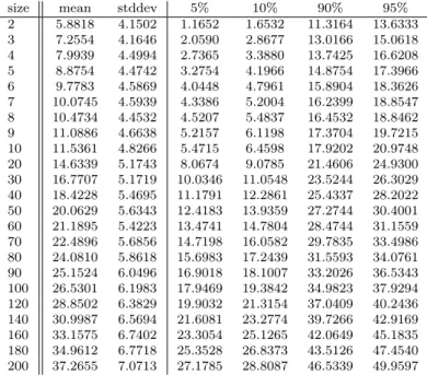
Table 1 shows the sample quantiles of Tn when both Xi and Yi are two- dimensional standard normal. Each value is calculated for fixed n using 1000 replications. The upper quantile values (at90% or 95%) can serve as critical val- ues for the test

H0 : Xi is two-dimensional standard normal.

Table 2 contains the results when both samples are two-dimensional uniform (more precisely uniform on[0,1]×[0,1]).

3. The mixed case

With the help of previous section’s tables one can construct empirical confidence intervals for the distance Tn of two samples both in the Gaussian-Gaussian and uniform-uniform cases. In what follows we present some results on the distance Tn for the Gaussian-uniform case. For this aim we performed calculations for sample sizesn= 2, . . . ,200with2000replications in each cases. Note that here we used U(−√

3,√

3) for the uniform variable because then we have E(Yij) = 0 and D²(Yij) = 1.

Figure 3 and Table 3 concern the distribution ofTnwhenXijis standard normal andYij ∈ U(−√

3,√

3). That is the case whenH0 is not satisfied. If we compare

the last columns (95% quantiles) of Table 3 and Table 1, then we see that our test is sensitive if the sample size is large (n≥100).

4. Fitting the GEV

To describe the distribution of Tn we fitted general extreme value distribution.

For each fixednwe estimated the parameters ofGEV from the1000replications.

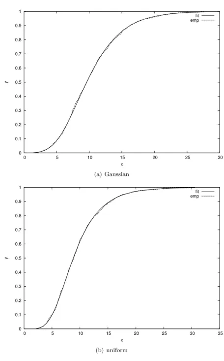
The maximum likelihood estimates of parametersξ, µ, σin (1.4) were obtained with MATLAB’sfitdistprocedure. Then we plotted the cumulative distribution function of the GEV. Figure 4(a), Figure 5(a) and Figure 6(a) show that the empirical distribution function of Tn fits well to the theoretical distribution function of the appropriateGEV when bothXiandYiare standard Gaussian. Figure 4(b), Figure 5(b) and Figure 6(b) show the same for uniformly distributedXi andYi.

Figure 7 shows the empirical significance of Kolmogorov-Smirnov tests per- formed by kstest. The empirical p-values in Figure 7(a) and Figure 7(b) reveal that the fitting was succesful.

5. About the GEV parameters

To suspect something about the possible ’analytical form’ of parametersξ, σ, µwe made further simulations in the Gaussian case with 5000 replications for sample sizes n= 2, . . . ,500. After several ’trial and error’ attempts we got the following experimental results.

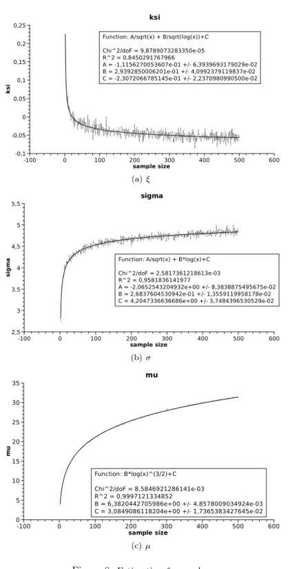
Figure 8 concern the functional form of the parameters. Here both Xi and Yi were Gaussian. For each fixed n we fitted GEV(ξ(n), σ(n), µ(n)). Then we approximatedξ(n), σ(n)andµ(n)with certain functions. For example we obtained thatξ(n)can be reasonably approximated with

A/√

n+B/p

log(n) +C

where A, B, C are given in Figure 8(a). Note that the classical goodness of fit measures (χ² andR²) computed byqtiplotindicate tight fit.

6. Tools

The Hungarian method was implemented inC++using the GNU g++ compiler.

Most of the graphs were made with the help of the utilitygnuplot. The fittings and the graphs of the last section were performed withqtiplot. MATLAB was used to compute the maximum likelihood estimators of theGEV.

7. Figures and tables

0 5 10 15 20 25 30

0 20 40 60 80 100 120 140 160 180 200

mean

size

gaussian

(a) Gaussian

4 6 8 10 12 14 16 18 20

0 20 40 60 80 100 120 140 160 180 200

mean

size

uniform

(b) uniform

Figure 1: Sample means

4.2 4.4 4.6 4.8 5 5.2 5.4 5.6 5.8 6 6.2

0 20 40 60 80 100 120 140 160 180 200

stddev

size

gaussian

(a) Gaussian

3 3.5 4 4.5 5 5.5 6

0 20 40 60 80 100 120 140 160 180 200

stddev

size

uniform

(b) uniform

Figure 2: Sample standard deviations

size mean stddev 5% 10% 90% 95%

1 4.2412 4.2266 0.2381 0.4563 9.8020 12.2026 2 5.9673 4.3135 1.0836 1.7158 11.7292 14.2147 3 7.4222 4.6192 1.7995 2.5588 13.7402 16.0102 4 8.0206 4.6088 2.3981 3.2674 13.6933 16.0876 5 9.3045 4.9715 3.2585 4.1318 15.3954 18.3475 6 10.2078 5.3420 3.7299 4.5396 17.1818 19.4804 7 10.3123 4.5427 4.1995 5.2007 16.2449 19.0637 8 11.0368 4.7393 4.8979 5.7742 17.5610 19.8337 9 11.5844 5.0128 5.0169 5.7831 18.2823 20.9534 10 12.0570 5.3378 5.3833 6.3622 19.4668 21.8923 20 15.2328 5.3538 8.6359 9.5934 22.2431 24.9313 30 16.9197 5.2032 10.1785 11.0722 23.9962 27.0184 40 18.3806 5.2547 11.4259 12.6406 25.5429 28.0519 50 19.9502 5.6199 12.1530 13.5418 27.2146 30.6897 60 20.4902 5.3926 13.3070 14.3950 27.5160 31.5666 70 21.7366 5.5615 14.3281 15.5132 28.9196 32.1283 80 22.2543 5.6370 14.6116 15.8363 29.4256 32.3583 90 23.0996 5.3942 15.7942 16.9445 30.0369 33.0472 100 23.1510 5.3759 15.9969 17.0670 29.9957 33.3124 120 24.9210 5.6381 16.9766 18.4435 32.5778 34.7392 140 25.7610 5.5036 18.1150 19.5019 33.0206 35.3015 160 26.1585 5.3739 18.7503 20.0962 33.6252 36.3843 180 27.3072 5.7067 19.4513 20.7716 34.7677 37.3559 200 27.7257 5.3810 20.2195 21.4550 34.8416 37.1973

Table 1: Quantiles. (a) Gaussian case

size mean stddev 5% 10% 90% 95%

1 4.0262 3.4236 0.1970 0.4216 9.1473 10.7406 2 5.7465 3.6683 1.1099 1.7597 10.9533 12.8762 3 7.0817 3.9889 1.9709 2.5498 12.4090 14.4607 4 8.0923 4.2833 2.5078 3.3816 13.7593 16.6473 5 8.7164 4.3022 3.0438 4.0823 14.4455 17.0613 6 9.2447 4.5952 3.4694 4.3526 15.5264 18.0257 7 9.6608 4.3776 4.1441 5.0191 15.5752 17.7570 8 10.2707 4.8150 4.3921 5.3208 16.7853 19.6646 9 10.5731 4.7847 4.6570 5.4796 16.7946 19.8556 10 10.7589 4.9081 5.0283 5.7636 16.9497 19.6734 20 12.9231 5.2142 6.8068 7.5361 19.3753 22.0094 30 13.6183 4.9743 7.7449 8.5648 20.3468 23.5615 40 14.3316 5.3870 7.9332 9.0030 21.1094 24.8500 50 15.0187 5.2400 8.8329 9.6225 21.8464 25.6322 60 15.2523 5.2565 8.9552 9.8825 21.8732 25.0060 70 15.8911 5.3841 9.5833 10.5137 22.9240 26.1478 80 15.8035 5.0754 9.7065 10.5853 22.9256 26.3499 90 16.2536 5.2216 9.9975 10.7825 22.9050 26.0921 100 16.4830 5.3264 10.2617 10.8682 24.0967 27.2588 120 17.0734 5.6685 10.4419 11.3588 24.4638 28.9698 140 17.2442 5.6141 10.7627 11.5904 24.3573 27.6821 160 17.5099 5.4433 11.1689 12.0155 24.9285 27.9288 180 17.5731 5.4062 11.1337 12.0112 24.5775 27.8075 200 18.0244 5.6245 11.4052 12.3776 25.4038 28.4148

Table 2: Quantiles. (b) uniform case

size mean stddev 5% 10% 90% 95%

2 5.8818 4.1502 1.1652 1.6532 11.3164 13.6333 3 7.2554 4.1646 2.0590 2.8677 13.0166 15.0618 4 7.9939 4.4994 2.7365 3.3880 13.7425 16.6208 5 8.8754 4.4742 3.2754 4.1966 14.8754 17.3966 6 9.7783 4.5869 4.0448 4.7961 15.8904 18.3626 7 10.0745 4.5939 4.3386 5.2004 16.2399 18.8547 8 10.4734 4.4532 4.5207 5.4837 16.4532 18.8462 9 11.0886 4.6638 5.2157 6.1198 17.3704 19.7215 10 11.5361 4.8266 5.4715 6.4598 17.9202 20.9748 20 14.6339 5.1743 8.0674 9.0785 21.4606 24.9300 30 16.7707 5.1719 10.0346 11.0548 23.5244 26.3029 40 18.4228 5.4695 11.1791 12.2861 25.4337 28.2022 50 20.0629 5.6343 12.4183 13.9359 27.2744 30.4001 60 21.1895 5.4223 13.4741 14.7804 28.4744 31.1559 70 22.4896 5.6856 14.7198 16.0582 29.7835 33.4986 80 24.0810 5.8618 15.6983 17.2439 31.5593 34.0761 90 25.1524 6.0496 16.9018 18.1007 33.2026 36.5343 100 26.5301 6.1983 17.9469 19.3842 34.9823 37.9294 120 28.8502 6.3829 19.9032 21.3154 37.0409 40.2436 140 30.9987 6.5694 21.6081 23.2774 39.7266 42.9169 160 33.1575 6.7402 23.3054 25.1265 42.0649 45.1835 180 34.9612 6.7718 25.3528 26.8373 43.5126 47.4540 200 37.2655 7.0713 27.1785 28.8087 46.5339 49.9597

Table 3: Quantiles. Gaussian-uniform case

Gaussian-uniform mean-stddev

Y

0 5 10 15 20 25 30 35 40

sample size

0 50 100 150 200 250

mean

stddev

Figure 3: Sample means and standard deviations, Gaussian-uniform case

0 0.1 0.2 0.3 0.4 0.5 0.6 0.7 0.8 0.9 1

0 5 10 15 20 25 30

y

x

fit emp

(a) Gaussian

0 0.1 0.2 0.3 0.4 0.5 0.6 0.7 0.8 0.9 1

0 5 10 15 20 25 30 35

y

x

fit emp

(b) uniform

Figure 4: Empirical and fitted cdf,n= 7

0 0.1 0.2 0.3 0.4 0.5 0.6 0.7 0.8 0.9 1

10 15 20 25 30 35 40 45 50 55

y

x

fit emp

(a) Gaussian

0 0.1 0.2 0.3 0.4 0.5 0.6 0.7 0.8 0.9 1

5 10 15 20 25 30 35 40 45 50 55

y

x

fit emp

(b) uniform

Figure 5: Empirical and fitted cdf,n= 77

0 0.1 0.2 0.3 0.4 0.5 0.6 0.7 0.8 0.9 1

15 20 25 30 35 40 45 50 55

y

x

fit emp

(a) Gaussian

0 0.1 0.2 0.3 0.4 0.5 0.6 0.7 0.8 0.9 1

5 10 15 20 25 30 35 40 45

y

x

fit emp

(b) uniform

Figure 6: Empirical and fitted cdf,n= 177

0 0.1 0.2 0.3 0.4 0.5 0.6 0.7 0.8 0.9 1

0 20 40 60 80 100 120 140 160 180 200

empsig

size

gaussian

(a) Gaussian

0 0.1 0.2 0.3 0.4 0.5 0.6 0.7 0.8 0.9 1

0 20 40 60 80 100 120 140 160 180 200

empsig

size

uniform

(b) uniform

Figure 7: Empirical significance

ksi

ksi

-0,1 -0,05 0 0,05 0,1 0,15 0,2 0,25

sample size

-100 0 100 200 300 400 500 600

Function: A/sqrt(x) + B/sqrt(log(x))+C Chi^2/doF = 9,8789073283350e-05 R^2 = 0,8450291767966

A = -1,1156270053607e-01 +/- 6,3939693179029e-02 B = 2,9392850006201e-01 +/- 4,0992379119837e-02 C = -2,3072066785145e-01 +/- 2,2370980990500e-02

(a)ξ sigma

sigma

2,5 3 3,5 4 4,5 5 5,5

sample size

-100 0 100 200 300 400 500 600

Function: A/sqrt(x) + B*log(x)+C Chi^2/doF = 2,5817361218613e-03 R^2 = 0,9581836141977

A = -2,0652543204932e+00 +/- 8,3838875495675e-02 B = 2,6837604530942e-01 +/- 1,3559119958178e-02 C = 4,2047336636686e+00 +/- 3,7484396530529e-02

(b)σ mu

mu

0 5 10 15 20 25 30 35

sample size

-100 0 100 200 300 400 500 600

Function: B*log(x)^(3/2)+C Chi^2/doF = 8,5846921286141e-03 R^2 = 0,9997121334852

B = 6,3820442705986e+00 +/- 4,8578009034924e-03 C = 3,0849086118204e+00 +/- 1,7365383427645e-02

(c)µ

Figure 8: Estimatingξ,σandµ

Acknowledgement. I would like to thank Prof. István Fazekas who suggested usingGEV to this problem.

References

[1] M. Ajtai, J. Komlós, G. Tusnády, On optimal matchings, Combinatorica, 4(4):259–

264, 1984.

[2] I. Fazekas, A. Roszjár, On test of two dimensional normality,Technical Report, Univ.

of Debrecen, 153, 1995.

[3] E.G. Gol’shtein, D.B. Yudin, Problems of linear programming of transportation type, (Russian), Nauka, Moscow, 1969.

[4] N. Henze, Invariant tests for multivariate normality: A critical review, Stat. Pap., 43(4):467–506, 2002.

[5] S. Kotz, S. Nadarajah, Extreme value distributions. Theory and applications,Imperial College Press, London, 2000.

[6] M. Talagrand, The generic chaining. Upper and lower bounds of stochastic processes, Springer, Berlin, 2005.

[7] J.E. Yukich, Optimal matching and empirical measures, Proc. Am. Math. Soc., 107(4):1051–1059, 1989.