Methods for Optimising Operation of Heterogeneous Networks

(1)

Methods for Optimising Operation of Heterogeneous Networks

— D.Sc. Dissertation —

In partial fulfillment of the requirements for the title of

“Doctor of the Hungarian Academy of Sciences”

Tibor Cinkler

HSNLab(High-Speed Networks Laboratory)

TMIT (Department of Telecommunications and Media Informatics) BME (Budapest University of Technology and Economics)

Magyar tudósok körútja 2., H-1117 Budapest, Hungary Tel.: +36-1-4631861; E-mail: cinkler@tmit.bme.hu

Budapest, 2012

(2)

(3)

Gyermekeimnek, Jolán Borbálának és Soma Zsoltnak, akik az ihlet és a boldogság kimer´ıthetetlen forrásai voltak minden pillanatban...

Edesanyámnak és ´´ Edesapámnak, negyvenegynéhány éves bizalmukért, hitükért és a biztos hátországért...

III

(4)

(5)

Acknowledgements

First of all I wish to thank to all my co-authors, mostly my former or current PhD students all the work we did together. Without them I could never complete this amount of work. In most of the cases they carried out the numerical evaluations and simulations. Special thanks go to János Tapolcai, János Szigeti, Péter Soproni, Marcell Perényi, Péter Laborczi, Gábor Rétvári, Szilárd Zsigmond, András Kern, Péter Hegyi, Attila Mitcsenkov and László Gyarmati. This order follows mostly the number of publications we had together. Words of thanks go to my colleagues József B´ıró, István Moldován and Krisztián Németh. I am also grateful to MSc students Géza Geleji, Dénes Gál and Réka Szabados. They also did useful simulations. Thanks go to all other co-authors as well, whom I did not list here.

I am grateful to Professors Lajtha, Sallai and Henk for their encouragements to complete this work, that started a few minutes after my PhD defence in 1999.

I am grateful to Tamás Henk, Gyula Sallai and Róbert Szabó, the management of the HSNLab and of the TMIT, for their encouragement. I am also grateful to Tamás for not letting me go for the Lab-skiing this year.

I wish to thank all the friendly encouragements to colleagues József B´ıró, Gyula Csopaki, Vilmos Simon and Péter Baranyi.

A word of thanks is also due Alpár Jüttner and Michal Pióro for fruitful discussions.

Very special thanks go to Ericsson for their generous support of my work, as well as to the companies (Magyar Telekom, Pantel, Alcatel-Lucent, Netvisor, Elsinco) we colaborated with, and to many Foundations and Scholarship Programs including MTA Bolyai and OTKA Postdoctoral Scholarship, for financially supporting me and my work during my postdoc research and for giving me the opportunity to travel to present my results and make contacts.

Words of thanks go to all colleagues we worked together for seven years in European research programs NOBEL, NOBEL II, e-Photon/ONe, e-Photon/ONe+, BONE, PROMISE, TIGERII, COST 266, 291 and 293.

I am grateful to my roommates, G´eza Paksy for his always wise advices and his help in all areas of technology and everyday life, I learned much from him; and to Ivett Kullik whom I partially owe my English exam, and who did not allow anyone to disturb me unnecessarily while working.

I wish to thank to Erika Szabó and András Balázs (MTA) their help around submitting my work to MTA as well as to Edit Halász, Györgyi Koroknai, István Kollár and Erzsébet Budai (BME) in updating the publication database with citations.

I am grateful to all colleagues of the Lab and of the Department for the nice and inspiring atmosphere.

Finally, I wish to thank my Mother, Father and Brother for their never-ending and unexhaustable trust, confidence and support.

I am grateful to the lady of my heart for her patience, sustainment and understanding in the last few “seven working days”.

V

(6)

(7)

“Per aspera ad astra!”

,,Az élet semmit sem ad a halandónak munka nélkül.”

Seneca

“Nullus agenti dies longus est.”

Seneca

,,Mondottam, ember küzdj és b´ızva b´ızzál!”

Madách Imre: Az ember tragédiája

,,Dolgozni csak pontosan, sz´epen, ahogy a csillag megy az ´egen,

´ugy ´erdemes.”

J´ozsef Attila

,,Hass, alkoss, gyarap´ıts:

s a haza f´enyre der˝ul!”

K¨olcsey Ferenc: Huszt

,,Semmilyen sz´el nem kedvez annak, aki nem tudja, melyik kik¨ot˝obe tart.”

Seneca

VII

(8)

(9)

List of Figures

1.1 Illustration of the Shared vs. Dedicated Protection when some working paths share

the risk of a single failure. . . 2

1.2 Link-, Segment-, and End-to-end Path Protection. . . 3

1.3 Comparing blocking ratios of five different protection methods to the GSP as the load increases in the network by scaling up the bandwidth b of demands. . . 5

1.4 Three Capacity Cost Models for Protection Paths . . . 7

1.5 How to calculate the Capacity allocated for Shared Protection? . . . 7

1.6 Illustration of the Link Duplication . . . 8

1.7 The blocking ratios of the three methods for three networks as the network capacity increases. . . 13

1.8 The running time average expressed in seconds on a logarithmic scale for the three methods for three networks. . . 14

1.9 The average network utilisation by working and protection paths for the three methods for the three networks. . . 14

1.10 Throughput of six test networks assuming eight cases with three fairness definitions. 21 1.11 Values for throughput and minα resulted by methods SPA, EISA (IESA) and EILP assuming protection types MWP and MBP . . . 23

1.12 Values for minα while decreasing link capacities with the following protection types: without protection (NP), Maximize Working Path with dedicated protection (MWP- DP), Maximize Working Path with shared protection (MWP-SP) and Maximize Both Paths (MBP). . . 23

1.13 Handling Inter-Domain Link Failures . . . 24

1.14 Logical internal p-cycle connections and alternate resolutions . . . 25

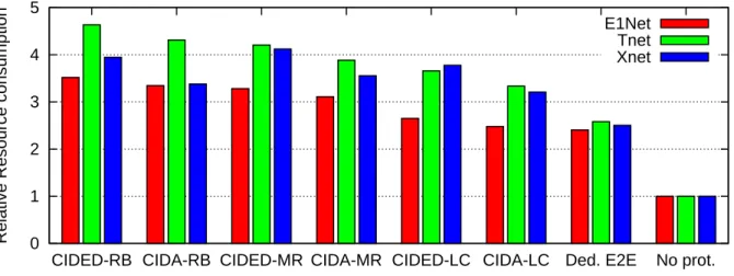
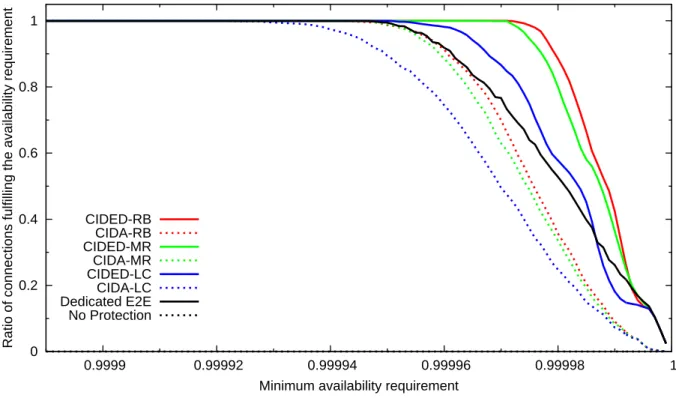
1.15 Resource requirement of protection schemes compared to the case of No Protection . 25 1.16 Tail behaviour of protection schemes in Tnet . . . 26

1.17 Illustration of the MPP problems: working + protection bandwidth allocations for certain two, three and four disjoint paths. . . 26

1.18 xy_max the required total protection capacity relative to the total working one as the number of disjoint paths grow: Theoretical result where all the paths are assumed to have the same length and the same allocation. . . 27

1.19 Comparing the blocking ratio of MPP to DPP and SPP for the COST 266 network as the capacity is scaled up of increasingly dense networks. . . 30

1.20 The trade-off between resource requirements and unavailability level. . . 31

1.21 What ratio of connections and why can satisfy a certain availability level? . . . 32

2.1 Modelling edges in the graph model. . . 37

2.2 Model of OADM nodes. . . 38

2.3 Model of EOXC nodes. . . 38

2.4 Simple OXC (no λ-conversion). . . . 38

2.5 OXC withλ-conversion. . . . 38 XIII

(14)

2.6 Relative frequency histogram of the number of free (unused) ports. Examples for

under-utilised (left), optimally utilised (middle) and over-utilised (right) nodes. . . . 45

2.7 Relative frequency histogram of the free capacity of links. Example for a lightly (left) and for a heavily (right) utilised link. . . 46

2.8 Network-level blocking ratio as a function of the per node blocking threshold T_N (left) and the required total number of grooming ports as a function of network-level blocking ratio (right). . . 48

2.9 Network blocking ratio as a function of the per link blocking threshold (left) and the required total number of wavelengths as a function of network blocking ratio (right). 49 2.10 The total number ofports in the network vs. the iteration steps. . . 50

2.11 The total number ofwavelengths as a function of iteration steps. . . 51

2.12 An example for fragmentation of λ-paths when new demands arrive that would be otherwise blocked in case with no fragmentation. . . 52

2.13 A grooming capable node to be modelled as a FG. . . 53

2.14 Routing with grooming in the FG that models 3 nodes. . . 70

2.15 FG when simple grooming is assumed: a) A demand of bandwidthb₁ is routed using the shown edge costs; b) after routing a demand the costs and capacities are set - all alternative links are disabled except one. . . 70

2.16 FG when the proposed method is used: b) After routing a demand all alternative links are allowed (“shadow links”), but their costs include cost of fragmentation as well. . . 70

2.17 If routing a new demand of bandwidthb₂over the shadow links in the FG theλ-paths will be cut (fragmented) by temporarily disabling (deleting) the internal optical link. 70 2.18 The NSFnet topology. . . 71

2.19 Blocking ratio against the ratio of the demand bandwidth to the channel capacity for the NSFnet and for the COST266BT networks. . . 72

2.20 Blocking ratio against the average connection holding time for the NSFnet and for the COST266BT networks. . . 72

2.21 Blocking ratio against the number of wavelengths for the NSFnet and for the COST266BT networks. . . 72

2.22 Comparing blocking performance of the simple grooming and of the proposed adaptive grooming as the level of traffic changes. . . 73

2.23 Comparing blocking performance of the CP/CP to the CP/MP model as the level of traffic changes (’freeze’ at 2000; increase traffic at 4000; ’melt’ at 6000, decrease the traffic at 8000; ’freeze’ at 10000). . . 73

2.24 Hop-count histogram for the case of connection arrival intensity of 0.01 for the three methods (simple, CP/CP and CP/MP). . . 73

2.25 Hop-count histogram for the case of connection arrival intensity increased by 20% (0.012) for the three methods (simple, CP/CP and CP/MP). . . 73

2.26 Blocking ratio for OGS vs. theλ-path tailoring OGT model. . . . 74

2.27 Relative gain of OGT over OGS. . . 74

2.28 Physical andλHop-Count as a function of bandwidth. . . 74

2.29 Blocking ratio as a function of bandwidth. . . 74

2.30 Physical andλHop-Count as a function of the distance. . . 74

2.31 Blocking ratio as a function of the distance. . . 74

2.32 Edge weights . . . 75

2.33 The value of parameter a. . . . 75

2.34 The value of parameter b. . . . 75

2.35 The results. The x-axis shows the expected value of the holding time (i.e. the network load). The legend is only shown in the first row, but applies to the rest too. . . . 76

(15)

2.36 The COST 266 reference network and various simulation results, all shown as the offered traffic decreases (horizontal axis). The results for protection paths of Dedicated

and Shared Protection overlap in Figures 2.36(e) and 2.36(f). . . 77

2.37 The results of simulating failures and recovering after them using four methods: ASP, ASP partial, ILP, ILP partial. The triple columns show the three methods ASP, MPH and ILP for setting up trees initially. The left-most triplet of columns is the failureless reference case in Figures 2.37(a)-2.37(f). . . 78

3.1 Illustration of the two PICR (Physical Impairment Constrained Routing) problems considered. . . 80

3.2 Dependence of the blocking on the network scale and grooming capacity (number of ports). . . 82

3.3 Blocking: Dependence on the network scale (’Expansion’) and grooming capacity (’Port number’). . . 83

3.4 Average per-demand hopcount: Dependence on the network scale (’Expansion’) and grooming capacity(’Port number’). . . 84

3.5 Average per-demand number of those regenerations that were required explicitly because of physical impairments: Dependence on the network scale (’Expansion’) and grooming capacity (’Port number’). . . 85

3.6 Maximum number of routed demands versus the n-factor for different scale parameters. 85 3.7 Base idea of PICR . . . 85

3.8 Maximum number of routed demands versus the n-factor for different number of wavelengths. . . 88

3.9 PICR (Physical Impairment Constrained Routing) of a single demand. . . 89

3.10 Simulation results forCost266BT (diameter 5051 km). Link weight models: Linear: the cost of a link is equal to its power load, Logarithmic: the cost is the natural logarithm of the load,Exponential: the cost iseraised to the load,Square: the cost is the square of the load, Breakline: the cost is the maximum of zero and the load minus maximum power multiplied by 0.8, Dijkstra: the cost is the link length. . . . 95

3.11 Work-flow for Protected PICR (P-PICR). . . 96

3.12 Routing ratio of demands . . . 96

3.13 Number of routed demands as a function of time step . . . 97

3.14 Ratio of routed demands as a function of inserted demand number . . . 97

3.15 Average routing time . . . 97

3.16 Routing of two demands between S2−T2 and S1−T1 respectively. The length and reserved power load is shown in curly brackets. We supposed linear dependence between the distance and power with 1 as factor, the maximum link power load is set to 40 units. . . 98

(16)

(17)

List of Tables

1.1 The illustration of the |B_ij^kl|matrix. . . 4 1.2 The properties of the networks and of the offered traffic. . . 12 1.3 Details of the six test networks. . . 20 1.4 Computational time [s] of ILP and IESA for six test networks and three protection

schemes . . . 21 2.1 Advantages of the Port- &λ-Shared Protection over the Capacity-Shared Protection. 64

XVII

(18)

(19)

Preface

This dissertation was submitted to the Hungarian Academy of Sciences in partial fulfillment of the requirements for the title of the “Doctor of the Hungarian Academy of Sciences”.

It summarises my results on routing, multicasting, traffic engineering and resilience in multi- layer and multidomain optical-beared modern transport networks achieved during my post-doctoral research. I have proposed models and algorithms for the above problems. The results are presented in Chapters 1, 2 and 3 in more details, they are summarised in Chapter 4 in 3 pages, while the booklet of theses lists the results with short explanation in roughly 6 pages in Hungarian.

Chapter 1 consists of results on resilience. It presents various approaches to reduce resource requirements while maintaining high level of availability.

Chapter 2 presents results related to grooming in two-layer networks. Models, ILP formulations and algorithms are presented.

Chapter 3 deals with methods for PICR, Physical Impairment Constrained Routing.

The results described in the dissertation can be efficiently used as a support tool for control or management of networks.

XIX

(20)

(21)

Chapter 1 Resilience of Networks

1.1 Introduction

In infocommunications networks there appear new applications all the time that face the network operators with new needs including the ever increasing requirement for higher availability.

Just to mention some examples. The electronic payment and the banking system must be always available, our VoIP systems as well as telephone systems must be always usable, our virtualised, often web based office applications, stored files, data centers and cloud computing facilities must be always accessible, not mentioning the high definition video contents where not only interrupts but also quality deteriorations are not tolerated by the users.

The problem is that the networks became rather heterogeneous, including the data plane, as well as the management and control planes. Under heterogeneity we mean multiple layers (MLN:

Multi-Layer Network), multiple domains (MD), multiple networking technologies (MRN: Multi- Region Network) and protocols, multiple services and QoS requirements, multiple vendors, etc. In such heterogeneous, and therefore rather complex networks it is rather hard to satisfy the high availability expectations in a simple, scalable, cost-effective way.

1.1.1 On Availability

When guaranteeing availability of “four nines”(0.9999), “five nines” (0.99999) or “six nines”(0.999999) that are availability levels often required in practice the network is unavailable for up to 52.56 minutes, a bit over five minutes (5 min 15.36 sec) or a bit over half a minute (31.536 sec) respectively during a whole year! This can be not kept by repairing the failed network components upon a failure. The network must be equipped with mechanisms that “heal” the failed parts of the network by automatically bypassing failed components. The de facto standard for restoring network services upon a failure is 50 ms. This value was defined for SDH/SONET networks, however, it is now a requirement for all networks. The objective is to guarantee this value, in the most cost effective way. I.e., to use few resources to save CAPEX or to use very simple mechanisms to save the OPEX.

1.1.2 On Resilience

The termResiliencecovers those schemes or mechanisms that make the network recover its services in short time upon a failure.

1.1.3 Protection or Restoration?

These mechanisms are traditionally classified into Protection and Restoration mechanisms. The difference is that while protection mechanisms have protection resources allocated in advance, and protection paths or segments of protection paths assigned to the resources the restoration schemes have typically no assigned protection paths, but they rather operate over instantly available free resources. The consequence of the operation is that protection works faster, however, requires

1

(22)

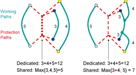
Figure 1.1: Illustration of the Shared vs. Dedicated Protection when some working paths share the risk of a single failure.

typically more resources. Restoration is typically slower, needs more complex control, however, it is more flexible, can restore typically multiple failures, and requires less data plane network resources.

We will focus mostly onto protection schemes in this chapter.

1.1.4 Dedicated or Shared?

From the point of view of resource utilisation the protection schemes can be classified into Shared and Dedicated. In case of Dedicated each working path has a protection one, typically with the same capacity allocated along it. In case of 1+1 Dedicated Protection, sometimes referred to as

“hot stand-by” the traffic is sent from the source along both paths, and the receiving end decides which signal to use. The 1:1 or “could stand-by” approach assumes that both, the sending and the receiving end have to switch to the protection path in any case the working path is affected. Here we will focus to theShared Protectionschemes, where we assume that a single failure can be present in the network at a time, and therefore any two working paths that have no element in common can share a protection path or a segment of a protection path, since either one or the other working path will need it, but never both of them, therefore, it is sufficient to allocate resources for the larger one only.

Figure 1.1 illustrates these cases. On the left hand side figure all three working paths having capacity requirements of 5, 3 and 4 respectively can share a protection path segment, since they have no element in common. Therefore 5 units of capacity instead of 12 are sufficient for shared protection in contrast to dedicated protection. However, if two paths have any element that can fail at the same time, then they belong to a Shared Risk Group (SRG) (in this case Shared Risk Link Group (SRLG)) and the sum of these two paths has to be considered in evaluating protection allocations as illustrated in the left hand side of Figure 1.1.

1.1.5 Path, Segment or Link?

Next we discuss the scope of protection. There are three cases.

First, when we protect each working path by a single protection end-to-end path that is completely disjoint from the working one (only the source and the target nodes are common) [97, 11].

In Figure 1.2 this protection scope is illustrated by a dashed-dotted thin line marked as “end-to-end / path”. In this case the strong disjointness is illustrated when there is neither link (edge, arc), nor node (vertex) in common for the working-protection path pair. In weaker sense it is sufficient if no common links are present. Regardless which element of the working path will fail, the same protection path will be used. This is a failure independent scenario.

(23)

segment

end−to−end / path link

S T

Figure 1.2: Link-, Segment-, and End-to-end Path Protection.

Second, when each link (or each element in general) of the working path has its own protecting bypass, typically one or more links, i.e., a segment. In Figure 1.2 this protection scope is illustrated by a dashed thin line marked as “link”. Clearly, this is a failure dependent scenario. Ring protection and p-Cycle protection are typical examples of link protection. Local control is sufficient, the protection is very fast, however, it typically uses more network resources than path protection.

Third, when two or more links have a common protection path segment is the tradeoff between path and link protection. This is illustrated by a thin dotted line in Figure 1.2 marked as “segment”.

In this case not only the different working paths can share protection resources, but also the multiple segments or links of a single working path can mutually share protection resources, since these segments are mutually disjoint [43].

1.1.6 The Structure of the Chapter

This Chapter on Resilience is structured as follows. In Section 1.2 a lower bound on the cost (resource requirement) of any shared protection scheme is provided. In Section 1.3 a resilience method is proposed that reoptimises all the protection resources together with the working and protection paths of any new demand. Section 1.4 proposes two new schemes for routing elastic traffic with protection along with a new fairness definition referred to as relative fairness. Section 1.5 presents two different approaches for performing shared protection in a multi-domain environment, where no sufficient information is available for sharing resources.

1.2 GSP: Generalised Shared Protection

GSP gives the bound on the Best Single-Demand Generalised Shared Protection. It finds for each demand the best general shared protection, regardless weather it is link-, segment- or end-to-end path-protection. Therefore, we will refer to it as GSP, the Generalised Shared Protection. This is a very good reference method for routing and protecting a single demand in most cost efficient way.

Since its ILP formulation is quite simple we provide it here.

1.2.1 ILP Formulation of the GSP

LetN(V, E, B^{f ree}) be a network defined by verticesv ∈V; edgese(i, j)∈Ewherei, j ∈V; and free bandwidths (or capacities) on edges e: b(e) ∈B^{f ree} where e∈E. B^{f ree} is the vector of currently available free capacities over all links e, i.e., if some demands are already routed over linksetheir bandwidth is subtracted from the capacity of that link.

Let (s, t, b) define the demands to be routed with GSP protection scheme. s is the source,t is the target (destination) of demands, whileb is their bandwidth requirement. We assume routing a single demand at time.

Let |B_ij^kl| be the matrix of extra bandwidth requirements for generalised shared protection of a demand having bandwidth requirement b as illustrated in Table 1.1. Each value of B_ij^kl in the matrix expresses how much additional bandwidth has to be allocated for protecting a demand over link ij that uses link kl in its working path by GSP. This conditional knowledge will help us to route simultaneously both, the working and the protection paths of a single demand.

(24)

Table 1.1: The illustration of the|B_ij^kl|matrix.

1 2 3 · · · kl · · · |E|

1 2

3... ...

ij · · · B_ij^kl · · ·

... ...

|E|

Here we define the variables, the objective and the constraints of the ILP (Integer Linear Pro- gram) or more precisely of the MILP (Mixed Integer Linear Program).

Variables:

xij ∈ {0,1} working flow over edgeij∈E

y_ij^kl∈ {0,1} protection flow over edgeij∈Ethat corresponds to the working flow over edgekl∈E, i.e., (ij, kl)∈E²

B_ij^max∈R is a real variable that expresses the amount of protection capacity to be used over link ij in optimal case

Objective:

min



b X

∀ij∈E

xij+α X

∀ij∈E

B_ij^max+β X

∀ij∈E

X

∀kl∈E\{ij}

y^kl_ij



 (1.1)

The first term minimises the total bandwidth used by the working path, the second term minimises the total bandwidth allocated for GSP protection, while the third term expresses the total number of links used by protection segments and protection paths . Consequently these three terms have to be weighted adequately. We assume that the first term has weight of 1 assigned, the second term has a value of 0< α <1 typically 0.5< α <0.9 to slightly prioritise the working to protection paths, and the weight of the third term is 0< β¿1 where it should have an infinitesimal value just to avoid accidentally nonzero y variables. By increasing β we will force protection paths become shorter and fewer, that leads sooner or later to end-to-end path protection instead of link or segment protection. Setting the value ofβ to zero the third term will be neglected. Then the objective will minimise the total capacity only.

Subject to:

X

∀k∈E^→l

xkl− X

∀m∈E^l→

xlm=





−1 ifl=s 0 otherwise 1 ifl=t

∀l∈V (1.2)

X

∀h∈E^→i,hi6=kl

y^kl_hi− X

∀j∈E^i→,ij6=kl

y^kl_ij =





−xkl ifi=s 0 otherwise xkl ifi=t

∀i∈V,∀kl∈E (1.3)

y^kl_ijB_ij^kl≤B_ij^max ∀kl∈E, kl6=ij,∀ij∈E (1.4)

xijb+B_ij^max≤B_ij^{f ree} ∀ij ∈E (1.5)

(25)

Figure 1.3: Comparing blocking ratios of five different protection methods to the GSP as the load increases in the network by scaling up the bandwidthb of demands.

1.2.2 Results

The results are shown in Figure 1.3. GSP is compared to five other protection methods:

• SPP: Shared Path Protection;

• SLP: Shared Link Protection;

• SPP-LR: SPP with LEMON Routing library [67] combinatorial solution;

• SSP: Shared Segment Protection;

• FDPP: Failure Dependent Path Protection.

It is interesting to note, that although GSP routes in any case the demand in most cost efficient way, in longer term in some cases it has suboptimal performance, since although all the protection paths are cheapest possible, they are often quite long, because they use those links for protection where no extra capacity is needed. In short term this thrifty scheme is advantageous, however, in longer term it uses to many resources and leads to blocking when the network is filled. All the numerical results were obtained running ILOG CPLEX [49] at our department computers and GNU GLPK [36] on supercomputers for solving the ILPs. The considered network was the COST266BT reference network, and the traffic was increased by increasing the ratio of its bandwidth to the link capacity from 3.8 to 6.6.

1.3 Adaptive Shared Protection Rearrangement

I propose a new approach with two algorithms for dynamic routing of guaranteed bandwidth pipes with shared protection that provide lower blocking through thrifty resource usage.

(26)

We assume that a single working path can be protected by one or multiple protection paths, which are partially or fully disjoint from the working path. This allows better capacity re-use (i.e., better capacity sharing among protection paths). Furthermore, the resources of a working path affected by a failure can be re-used by the protection paths.

The main feature of the proposed protection rearrangement framework is that since the protection paths do not carry any traffic until a failure they can be adaptively rerouted (rearranged) as the traffic and network conditions change. This steady re-optimisation of protection paths leads to lower usage of resources and therefore higher throughput and lower blocking.

The other novelty we propose in this paper is a modelling trick referred to as LD: Link Doubling that allows distinguishing the shareable part of the link capacity from the free capacity in case when multiple protection paths are being rerouted simultaneously. LD allows finding optimal routing of shared protection paths for the case of any single link failure!

The obtained results can be used for routing with protection in SDH/SONET, ngSDH/SONET, ATM, MPLS, MPLS-TP, OTN, Ethernet, WR-DWDM (including ASTN and GMPLS) and other networks.

This section is organised as follows. In Section 1.3.1 the problem is formulated, Section 1.3.2 presents the reference method used, while the idea of LD is presented in Section1.3.3. The two proposed methods are presented in Section1.3.4 and 1.3.5. Section 1.3.6 presents and evaluates the obtained numerical results.

1.3.1 Problem Formulation

The problem is how to optimally choose one working and one or more protection paths for a demand.

Here we formulate the problem and in the next section we propose methods for solving it.

According to the above definitions, our protection methods

• are shared

• are adaptive

• operate on segments (sub-networks) that can be a single or multiple links long and are deter- mined when the protection paths are sought

• use partially disjoint paths

• guarantee survival of any single failure, but work for some multiple failure patterns as well.

The probability of having two independent failures in the network at the same time is low, even lower for two failures along the same path. Therefore, it is justified to share protection resources (Figure 1.1).

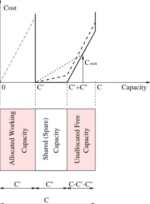
The algorithm for determining the amount of capacity to be allocated for backup paths in thrifty way, is based on the idea explained on Figure 1.1 [C36] . The capacityC_l of each linkl is divided into three parts (Figure 1.4):

1. C_l⁰ allocated to working paths;

2. C_l⁰⁰ allocated for (shared) protection (i.e., spare capacity); and 3. C_l−C_l⁰−C_l⁰⁰ the free, unallocated and unused capacity.

Given a network N(V, E, C) with nodes (vertices) v ∈ V, links (edges) e(v₁, v₂) ∈ E and link capacities C_l we want to satisfy all dynamically arriving (in advance unknown) traffic demands [C140] defined as a Traffic Pattern T(o :o(s_o, d_o, b_o, τ_o⁰, τ_o⁰⁰)) where b_o stands for the bandwidth of traffic demand o between source node s_o and destination node d_o that has arrived at time τ_o⁰, and lasts untilτ_o⁰⁰.

The working path P⁰(o) = (e⁰₁, e⁰₂, ...e⁰_|P0|) should be the shortest path with available capacity b_o. Another “shortest” path P_e⁰⁰0(o) = (e⁰⁰₁, e⁰⁰₂, ...e⁰⁰_|P00

e0|) is sought for each link e⁰ of the working path P⁰(o), that may fail, such thate⁰ ∈/P_e⁰⁰0.

“Shortest” means the path that requires the lowest resource allocation from theC −C⁰ −C⁰⁰ capacities (i.e. the lowest increment of C⁰⁰ capacities). The path is the shortest one in sense of the

(27)

CapacityUnallocated Free Allocated Working Capacity

C

0 C’ C’+C"

Csum

Capacity Cost

C

C’ C" C-C’-C"

Shared (Spare) Capacity

Figure 1.4: Three Capacity Cost Models for Protection Paths

capacity-cost functions shown in Figure 1.4. For routing the protection path for demand o that has bandwidth b_o we have to reserve on each link that amount of capacity only that exceeds the capacity that is shareable by the considered demand over the considered link. The sum of the costs of these non-shareable capacities for all the links along a path has to be minimal. This is the only metric we have used while routing. These paths P_e⁰⁰0(o) are referred to as partially disjoint, shared protection (PDSP) paths for pathP⁰(o).

. . . . . .

^A ^B ^D

B’ D’

A’

l’ l"

Figure 1.5: How to calculate the Capacity allocated for Shared Protection?

This problem can be formulated mathematically using graph theory and network flow theory.

Due to the complexity of the problem, we apply heuristics with the aim of being close to the global optimum. These heuristics include decomposition, approximations and modeling tricks.

(28)

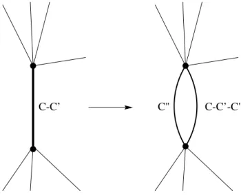
C-C’ C" C-C’-C"

Figure 1.6: Illustration of the Link Duplication 1.3.2 The Reference Method: Shared Path Protection (SPP)

As the reference we use the well known Shared Path Protection, where after routing the working path, we search for an end-to-end disjoint protection path that requires the lowest cost in the sense of the capacity cost function 1.4. We have to note here, that to avoid loops and overlengthy paths the shareable capacity was not for free, however, its unit capacity costed only a fraction of the cost of a unit of free capacity to be allocated. The same principle was used for all the evaluations in this section: the cost ratio was 1:10.

Here we briefly describe the Shared Path Protection algorithm:

The algorithm works as follows:

• Step 1: For the new demando_new: – Find the shortest working path.

– Delete (hide) temporarily all the links of the working path.

• Step 2: For all linksl⁰ of the working path:

– For all links l⁰⁰ of potential protection paths:

∗ Compute capacityC_l⁰_,l⁰⁰ required on linkl⁰⁰ when linkl⁰ fails (Figure 1.5 and 1.1).

• Step 3: Find the largest value C_l⁰⁰ ofC_l⁰_,l⁰⁰ for all l⁰ found so far.

• Step 4: Calculate the cost increment required for routing the protection path of bandwidth requirement b_o of demando_new according to figure 1.4 based on C_l⁰⁰ along all the links l⁰⁰ in the network.

• Step 5: Based on the cost increments obtained find the shortest protection path.

• Step 6: Store the new paths, deallocate resources for terminated connections, update the capacity allocations.

• Step 7: If more new demands arrive go to Step 1.

Shared Path Protection (SPP) is considered as a reference without the capability of rerouting (rearranging) the previously allocated protection paths. It is a really fast and easy solution for shared protection.

(29)

1.3.3 LD (Link Doubling)

In Section 1.3.2 we have presented the reference method, the SPP. Now we explain the idea of Link Doubling (LD) followed by the MILP formulation of Protection Re-arrangement and by our two proposed methods, namely Shared Path Protection with Link Doubling (SPP-LD) and Partially Disjoint Shared Path protection with Link Doubling (PDSP-LD).

Here we introduce LD, where LD stands for link doubling. LD is not an algorithm in itself but a modelling trick, however, it is the basis of the two proposed algorithms. First we explain why we need LD, then we explain how it works.

In a network that supports protection sharing, before routing the protection path of demando with bandwidth requirement b_o, we simply calculate the amount of capacity it would need over the shareable link. This capacity depends on two things. First, the amount of capacity of the demand exceeding the shareable part depends on the bandwidth b_o of that demand. Second, the allocated spare capacityC⁰⁰is not fully shareable by any demand, but typically only a part of it. Remember, that if two demands have a common linkl⁰ in their working paths, then they may not share capacity on linkl⁰⁰ (Figure 1.1).

One of the basic principles of our proposed methods is that we rearrange the protection paths, i.e., re-route them simultaneously. When we want to route protection paths of more than one demand simultaneously we face the above described problem. The bandwidth requirements of different demands will be different, and it will often happen that two or more protection paths that would share a link have a common link in their working paths. LD solves this problem.

In LD we use a modeling trick to be able to represent the two-segment cost function as shown in Figure 1.4 by solid line, or by the dashed line, to avoid unnecessarily long paths. Since the two segment capacity-cost function is a non-linear one we can neither use it in an ILP (Integer Linear Program) formulation, nor by the Dijkstra’s algorithm. Therefore, linearisation is needed.

The idea here is to use two parallel links (as shown in Figure 1.6) that both have linear capacity cost functions and represent the two segments of the cost function shown in Figure 1.4. The link representing the shared spare capacity will have capacity C⁰⁰ and the same or lower cost than the other link, which represents the free capacity C−C⁰−C⁰⁰.

The drawback is, that the number of links doubles in the worst case and therefore the runtime becomes longer, while the advantage is that we can get optimal result. Without LD an alternative would be to make a single segment linear approximation of the two segments, however, the result would be suboptimal.

For routing multiple shared protection paths an MILP (Mixed Integer Linear Programming) formulation is needed. Using LD the problem is linear and feasible.

MILP Formulation

In this section we present the MILP formulation of the problem of routing multiple shared protection paths simultaneously. The protection rearrangement means, that first we remove the considered protection paths from the network, recalculate all the free and shareable capacities and then we route all the removed paths and the new protection paths simultaneously as follows.

Objective:

min ^X

o∈Te



 X

l∈E^{f ree}

x^o_lw_l+ ^X

l∈E^sh

x^o_lγ_l



 (1.6)

Where E^sh is the set of all added (doubled) edges, with capacity C⁰⁰, representing the shareable part and E^{f ree} with capacity C−C⁰−C⁰⁰ being the set of edges that represent the remaining free capacity of all edges. Now E⁰=E^sh∪E^{f ree}. Note, thatE⁰ is the extended set of edges in contrast to E. Note, that the capacity used for working paths is not represented in this graph. If there is no shareable or no free capacity along a link, then the corresponding link can be left out from the LD-graph, the graph obtained by LD.

Here,γ_lrepresents the cost of a unit of capacity of the shareable spare capacity on linkl. It can take

(30)

values 0 ≤γ_l ≤w_l. If it is 0, then too long paths may appear. If it is equal to w_l then we do not prefer shareable to the free capacity at all. Extensive simulations have shown that the best results can be achieved by settingγ_l/w_l≈0.1,∀l∈E. Note, that herex^o_l is not a binary indicator variable, but it represents the amount of flow of demand o over link l. T_e is the set of those demands o for which we route simultaneously the shared protection paths. This set typically depends on an edge e that is within the working path of the demand that has been routed just before the protection path rearrangement is started. We will discuss the composition and meaning of the set T_e in more details when discussing algorithms SPP-LD and PDSP-LD.

Constraints: _X

o∈Te

x^o_l ≤C_l−C_l⁰−C_l⁰⁰ for all linksl∈E^{f ree} (1.7) X

o∈Te

x^o_l ≤C_l⁰⁰ for all links l∈E^sh (1.8)

X

∀j∈V,j6=i

x^o_ij − ^X

∀k∈V,k6=i

x^o_ki =







0 ifi6=s_o∧i6=d_o b_o ifi=s_o

−b_o ifi=d_o

for all nodes i∈V and demandso∈T_e (1.9) 0≤x^o_l ≤b_o for all links l∈E and demandso∈T_e. (1.10) X

∀k∈V,k6=i

xô_ki=b_o·z_iô for all nodes i∈V and demandso∈T_e. (1.11) z_iô ∈ {0,1} for all nodes i∈V and demandso∈T_e. (1.12) z_iô is an auxiliary binary variable (Eq.1.11). Its role is to avoid flow branching, while it allows flow splitting between the pairs of parallel edges of an adjacent pair of nodes (Eq.1.12), i.e., it models the LD. Equations (1.7) and (1.8) are the capacity constraints for free and shareable capacities, respectively. Equation (1.9) is the well known flow conservation constraint. Equation 1.10 is the non-negativity constraint and the upper bound of the flow.

Both SPP-LD and PDSP-LD use the MILP formulation of Link Doubling. The set T_e is the main difference between the SPP-LD and PDSP-LD.

1.3.4 SPP-LD: Shared Path Protection with Link Doubling

The basic idea of SPP-LD is that after routing the working path of demand o we do not route its protection path only, but also the protection paths of all the demands that have in their working paths any element (e.g., any link) in common with the working path of demand o. We do all this simultaneously.

The requirement is that there is a single end-to-end protection path for each demand othat is disjoint with the working path of that demand only, i.e., a protection path may use any link except those used by its corresponding working path. Protection paths can share resources except if they have any common link in their working paths.

However, routing all these demands simultaneously, and considering all constraints on disjointness of working and protection paths appeared to be extremely complex and not feasible in reason- able time.

Therefore, we have used an approximation of the above problem. We have decomposed the problem by relaxing the “all simultaneously” constraint, i.e., we consider the links of the working path one-by-one.

The algorithm works as follows:

• Step 1: For the new demando_new:

(31)

– Find the shortest working path.

• Step 2: For all the links eof the working path:

– Delete temporarily linke.

– Deallocate the protection paths of all the demandsothat use eas a part of their working paths.

– Set T_e to contain the new demand o_new and all the demands that used e as a part of their working paths.

– Execute the MILP for demands T_e with added path diversity constraints.

• Step 3: If more links ego to Step 2.

– Based on the knowledge of all working and protection paths currently present in the network calculate the capacity allocated for shared protection over all links.

• Step 4: If more new demands go to Step 1.

The path diversity constraint has not yet been discussed. It means, that a linkeis either used by the working path of demand o or by its protection path or by non of them, but never by both, the working and the protection. To avoid introducing new variables or by making real (continuous) variables binary (discrete) the simplest way was to simply leave out some of the variables that further decreased the complexity: If the working path of demand o uses link l then we leave out variable x^o_l completely from the MILP formulation for edges representing both, the shareable and the free part of the link capacities. Note, this holds for the new demand o_new as well, to have its protection completely diverse.

If a working path has more than one link in common with the working path of the new demand it can happen that it will have more than one protection path. In that case any of them can be chosen. For simplicity reasons we choose the latter found one. Then the capacities allocated for shared protection are calculated accordingly.

1.3.5 PDSP-LD: Partially Disjoint Shared Protection with Link Doubling The difference between SPP-LD and PDSP-LD is that while SPP-LD requires end-to-end disjoint protection paths, PDSP-LD will allow so-called partially disjoint paths as well. It means that we will allow protection paths to have common parts with the working one. However, to be able to protect the working path in case of failure of any of its links we must define more than one protection paths to cover all the failure cases.

As the numerical results show this leads to even better capacity sharing that results in better resource utilisation, while the complexity (and running time) of the algorithm is about the same as of SPP-LD.

The algorithm differs only in the last item of Step 2, i,e, MILP is executed without forcing path diversity, i.e., since link e is deleted all the protection paths will exclude it. In this case we define a protection scenario for each link of a protection path. Note, that it can happen that a path will be protected in the same way in the case of failures of its different links.

1.3.6 Numerical Results

The simulations were carried out on a Dual AMD Opteron 246 Linux server with 2 GBytes of memory. The code was written in C++, compiled by gcc 3.4.3 and the MILP solver was the ILOG CPLEX 9.030.

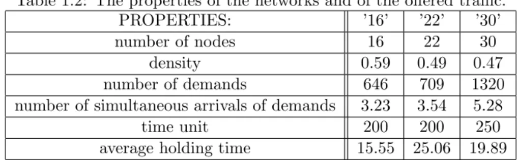
We have compared the performance of the three algorithms SPP, SPP-LD and PDSP-LD on three networks that consisted of 16, 22 and 30 nodes respectively. Table 1.2 shows the characteristics of the three networks and the characteristics of the traffic offered to these networks.

(32)

Table 1.2: The properties of the networks and of the offered traffic.

PROPERTIES: ’16’ ’22’ ’30’

number of nodes 16 22 30

density 0.59 0.49 0.47

number of demands 646 709 1320

number of simultaneous arrivals of demands 3.23 3.54 5.28

time unit 200 200 250

average holding time 15.55 25.06 19.89

To investigate different blocking ranges we have scaled the link capacities, not the traffic. Note, that increasing the capacity of every link uniformly is analogous to decreasing bandwidth of traffic offered to the network. We have investigated roughly the 0% to 90% blocking range. The number of demands that were routed was large enough to make the influence of the initial transient negligible.

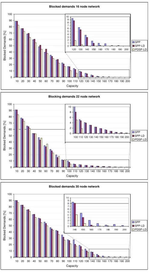
Figure 1.7 shows the blocking ratios of demands of the three algorithms on three networks. The blocking drops as the capacities of all the links were scaled up. SPP-LD had typically performance slightly better than SPP. PDSP-LD had always the best performance except for the 30-node network in the 50-60 % blocking range. The enlarged figures within the figures show the range of practical interest.

Figure 1.8 shows that the running time of SPP was much lower than that of methods using protection repacking (rearrangement).

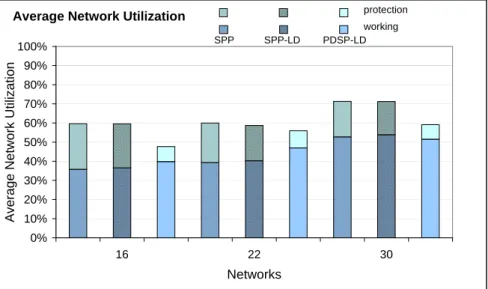
Figure 1.9 Shows the average network utilisation for the range, where the blocking of PDSP- LD was just below 1%. In all cases PDSP-LD used fewest resources. It is interesting to not, that although it has used typically slightly more resources for working paths it has used much less protection resources than the other two methods.

1.3.7 Remarks on PDSP-LD

In this section I have proposed re-arranging or re-packing protection paths to achieve better throughput. Re-arrangement makes no problem, since the protection paths do not carry any traffic. Second, we have introduced LD to linearise the two-segment capacity-cost functions.

The results show, that although the computational complexity has significantly increased it is still within boundaries of practical implementability for on-line routing. Both, the resource utilisation and the blocking ratios were better for PDSP-LD than for the SPP and for SPP-LD.

The ratio of protection resources obtained by PDSP-LD was particularly low, while it achieved up to 5% lower blocking than the other two methods.

1.4 Protected Elastic Traffic without Extra Capacity?

In infocommunications networks the available bandwidth typically varies in time. The transmission rate of theelastic trafficcan be tuned according to the actual network state. Assuming such elastic traffic there arises the problem how to allocate resources (bandwidth) to sources in a fair manner and how to protect connections against failures. In recent related works the paths of the demands are given in advance, consequently setting up elastic source rates in fair way leads to suboptimal solution. Better results can be achieved if we determine the bandwidth of elastic sources AND the routes used by these demands simultaneously. In several applications it is meaningful to define minimum and maximum rate for sources. For this case we propose the definition of Relative Fairness (RF).

In this section different resource allocation policies are formulated and algorithms proposed, supported by numerical results. Protection alternatives for elastic traffic are also discussed: two protection schemes are proposed and analyzed. The algorithms are compared assuming different

(33)

Figure 1.7: The blocking ratios of the three methods for three networks as the network capacity increases.

fairness definitions and different ways of handling protected elastic traffic. All the algorithms are a tradeoff (compromise) between network throughput, fairness and required computational time.

Nowadays, in infocommunications networks the rate of sources typically varies in time since

(34)

Figure 1.8: The running time average expressed in seconds on a logarithmic scale for the three methods for three networks.

Average Network Utilization

0%

10%

20%

30%

40%

50%

60%

70%

80%

90%

100%

16 22 30

Networks

Average Network Utilization

SPP SPP-LD PDSP-LD protection working

Figure 1.9: The average network utilisation by working and protection paths for the three methods for the three networks.

this guarantees higher throughput and better resource utilization. In non-real-time traffic of the Internet there is a growing interest in defining bandwidth sharing algorithms [87] which can cope with a high bandwidth utilization and at the same time maintain some notion of fairness, such as the Max-Min (MMF) [10, 15] or Proportional Rate (PRF) [60] fairness.

The most typical example of elastic traffic is the aggregate of TCP sessions in IP networks. The Available Bit Rate (ABR) Service Class in Asynchronous Transfer Mode (ATM) networks can be also mentioned. Label Switched Paths (LSPs) of Multiprotocol Label Switching (MPLS) networks are also easy to configure: their route and bandwidth can be adaptively changed. In all cases the source rates are influenced by the actual load of the network.

Three variants can be applied for determining the paths of elastic traffic : (1)fixed paths, (2) pre-defined paths, or (3)free paths. In the case offixed paths there is a single path defined between each origin-destination (O-D) pair and the allocation task is to determine the bandwidth assigned to each demand. In the case of pre-defined paths we assume that between each O-D pair, there is a set of admissible paths that can be potentially used to realize the flow of the appropriate demand.

In this case the allocation task does not only imply the determination of the bandwidth of the flow, but also the identification of the specific path that is used to realize the demands [34]. In the case of free paths there is no limitation on the paths, i.e., the task is to determine the bandwidth of the

(35)

traffic AND the routes used by these demands simultaneously. This novel approach, the joint path and bandwidth allocation with protection is the main topic of this section.

Recent research results indicate that it is meaningful to associate a minimum and maximum bandwidth with elastic traffic [70]; therefore, it is important to develop models and algorithms for such future types of networks. For the bounded elastic environment a special weighted case of MMF notion: Relative Fairness (RF) is proposed that maximizes the minimum rates relative to the difference between upper and lower bounds for each demand.

Considering literature different aspects of the max-min fairness policy have been discussed in a number of papers, mostly in ATM ABR context, since the ATM Forum adopted the max-min fairness criterion to allocate network bandwidth for ABR connections, see e.g. [47, 48]. However, these papers do not consider the issue of path optimization in the bounded elastic environment.

MMF routing is the topic of the paper [68], where the widest-shortest, shortest-widest and the shortest-dist algorithms are studied. These algorithms do not optimize the path allocation at all.

A number of fairness notions are discussed and associated optimization tasks are presented in [70]

for the case of unbounded flows and assuming fixed routes.

Proportional Rate Fairness (PRF) is proposed by Kelly [60] and also summarized by Massoulie and Roberts in [70]. The objective of PRF is to maximize the sum of logarithms of traffic bandwidths. While [60] does consider the path optimization problem, it does not focus on developing an efficient algorithm for path optimization when the flows are bounded.

Recent research activities focused on allocating the bandwidth of fixed paths. In [34] the approach has been extended in such a way that not only the bandwidth but also the paths are chosen from a set of pre-defined paths. The formulation of the pre-defined path optimization problem is advantageous, since it has significantly less variables than the free path optimization. However, its limitation is that the whole method relays on the set of pre-defined alternative paths. If the set of paths is given in advance, setting up elastic source rates in a fair way leads to suboptimal solution.

Better results can be achieved if we determine the rate of elastic sources AND the routes used by these demands simultaneously. There arises the question how much resources should be reserved for each demand, and what path should be chosen for carrying that traffic in order to utilize resources efficiently while obeying fairness constraints as well.

The protection against failures is an important issue also in case of elastic traffic since one portion (e.g., half, or the lower bound) of the traffic should be “alive” even if a network component is affected by a failure. To our knowledge, protection issues of elastic traffic have not been studied in the literature. Accordingly, we propose and analyze two types of protection schemes in elastic environment:

1. Maximize both, working and protection paths (MBP). In this case the traffic is routed on two disjoint paths of half-half capacity. If one of the two paths is affected by a failure then the bandwidth of the connection will be degraded to the half of the original.

2. Maximize working paths (MWP) - find any protection paths. In this case we aim to maximize the bandwidth of each traffic according to the fairness definitions while ensuring (whenever it exists) a disjoint protection path such that the system of working and protection paths fits into the capacity constraints with their lower bounds.

In case of a failure at least one pre-defined path remains active (“alive”) in case of either MBP or MWP. In case of MWP the bandwidths are set to the lower bounds, while with MBP will be halved, and augmented bandwidths can be calculated in a second phase of the recovery. Several questions arise: How fair are these protection schemes? How bandwidth-consuming they are? What amount of additional bandwidth do they need compared to the unprotected case?

In this section we investigate these questions and propose algorithms assuming three types of fairness definition: RF, MMF and PRF.

• Relative Fairness (RF): In this case the aim is, to increase the rates relative to the difference between upper and lower bounds for each demand.