Towards D-Optimal Input Design for Finite-Sample System Identification ?

Towards D-Optimal Input Design for Finite-Sample System Identification ?

S´andor Kolumb´an^∗ Bal´azs Csan´ad Cs´aji^∗∗

∗Department of Mathematics and Computer Science, Eindhoven University of Technology, Netherlands (e-mail: s.kolumban@tue.nl).

∗∗Institute for Computer Science and Control (SZTAKI), Hungarian Academy of Sciences, Hungary (e-mail: balazs.csaji@sztaki.mta.hu)

Abstract: Finite-sample system identification methods provide statistical inference, typically in the form of confidence regions, with rigorous non-asymptotic guarantees under minimal distributional assumptions.Data Perturbation (DP) methods constitute an important class of such algorithms, which includes, for example, Sign-Perturbed Sums (SPS) as a special case. Here we study a naturalinput designproblem for DP methods inlinear regressionmodels, where we want to select the regressors in a way that theexpected volumeof the resulting confidence regions are minimized. We suggest a general approach to this problem and analyze it for the fundamental building blocks of all DP confidence regions, namely, for ellipsoids having confidence probability exactly ¹/². We also present experiments supporting that minimizing the expected volumes of such ellipsoids significantly reduces the average sizes of the constructed DP confidence regions.

Keywords:system identification, confidence regions, finite sample results, least squares, parameter estimation, distribution-free results, input design

1. INTRODUCTION

Finite-sample system identification(FSID) methods infer properties of stochastic dynamical systems, arch-typically build confidence regions, with rigorous non-asymptotic guarantees under minimal statistical assumptions (Car`e et al., 2018). They are motivated, e.g., by results showing that applying asymptotic methods in finite sample settings can lead to misleading outcomes (Garatti et al., 2004).

Data Perturbation (DP) methods form a general class of FSID algorithms (Kolumb´an et al., 2015; Kolumb´an, 2016) which generalize the construction of the Sign-Perturbed Sums(SPS) method (Cs´aji et al., 2012, 2015; Kieffer and Walter, 2014; Weyer et al., 2017). While the core assump- tion of SPS is the distributional symmetry of the noise terms, DP methods can exploit other kinds of regularity and also work, for example, with exchangeable or power defined noise sequences. One of the key properties of DP methods is that, similarly to SPS, they are guaranteed to provideexact confidence regions (Kolumb´an, 2016).

Input design is a subfield of experiment design (Goodwin and Payne, 1977; Pintelon and Schoukens, 2012; Rodrigues and Iemma, 2014), and it is an important area of system identification, as the choice of the input signal has a substantial influence on the observations. There could be many possible aims of input design, for example, reducing the bias of the estimator, making the experiments more informative about some parts and modes, or minimizing the variance of certain components (Ljung, 1999).

? S. Kolumb´an was supported by the NWO Gravitation Project NETWORKS; B. Cs. Cs´aji was supported by the Hung. Sci. Res.

Fund (OTKA), KH 17 125698, the GINOP-2.3.2-15-2016-00002 grant, and the J´anos Bolyai Research Fellowship, BO/00217/16/6.

In this paper we study a natural input design problem for DP methods forlinear regressionmodels. Our aim will be to choose the inputs in a way that the expected volume of the constructed confidence regions is minimized. By arguing that all DP confidence regions can be built by unions and intersections of ellipsoids having confidence probabilityexactly¹/², we first analyze these ellipsoids, as they are the fundamental building blocks of DP regions.

Along the way we provide the first explicit formulation of these fundamental ellipsoids in terms of the regressor and perturbation matrices, the true parameter and the noise.

We show that minimizing their expected volume can be done by maximizing theexpected determinantof a certain quadratic term. This result has strong connections to classical D-optimal input design, but our method builds only on finite sample results and, hence it also depends on the actual regularity of the noise, i.e., the transformation group with respect to the distribution is invariant.

The paper ends with numerical experiments demonstrat- ing that minimizing the expected volume of such ellipsoids carries over to the general case and the resulting DP confidence regions have smaller volumes on average.

2. PRELIMINARIES

In this section we introduce some notations, formalize the model, and the input design problem for DP methods.

2.1 Notations

First, let us define a subset of positive integers up to and including a constantkas [k] , {1, . . . , k}. Thecardinality of a setS will be denoted by|S|. Thus,|[k]|=k.

For any matrix A, its transpose is denoted with A^T. In

denotes thendimensional identity matrix andkvkdenotes the Euclidien norm of a vector v, i.e., kvk² = v^Tv. We denote the set of alln×northogonalmatrices by

O(n) , {G∈R^n×n:G^TG=In}, (1) which forms agroupwith the usual matrix multiplication.

Given a (skinny, full rank) matrixA∈R^n×·, theorthogo- nal projectionmatrix to the column space ofAis

PA , A[A^TA]⁻¹A^T, (2) and the projection to itsorthogonal complementis

PA^⊥ , In−A[A^TA]⁻¹A^T. (3) Naturally, in both cases we haveP²=P andP^T=P. 2.2 Linear Regression

Let us consider the following linear regression problem

Y , Xθ0+E, (4)

whereX ∈R^n×nθ is the regressor matrix (i.e., the input), θ0∈R^nθ is an unknown (constant) true parameter vector, E∈Rⁿ is a random noise vector,Y ∈Rⁿ is the (random) vector of observations, and nis the sample size.

The classicalleast-squares(LS) method estimatesθ0given X andY. The LS estimate, ˆθn, can be written as

θˆn , argmin

θ∈R^nθ

kY −Xθk²= [X^TX]⁻¹X^TY, (5) ifX is skinny and full rank, which we assume henceforth.

As the LS estimate, ˆθn, depends on the random noiseE, it is a random vector. Confidence regions can be used to quantify the reliability of the estimate, but information about the distribution of E is required to construct such confidence regions. The most commonly used results are in this respect asymptotic (as n→ ∞), and build on the fact that, under mild statistical assumptions, we have

√n θˆn−θ0

_d

−→ N 0, σ²_eΨ⁻¹

, (6)

as n→ ∞, assuming the following covariance matrix Ψ , lim

n→∞

1

nX_n^TXn (7) exists and it is positive definite, where→^d denotes conver- gence in distribution, σ²e is the variance of the marginal distributions of the (homoskedastic) noise vector E, and N(µ,Σ) is the multidimensional Gaussian distribution with mean vectorµand covariance matrix Σ (Ljung, 1999).

Here we used an indexnfor the regressor matrix,Xn, to emphasize its dependence on the sample size.

A drawback of such asymptotic approaches is that they are not guaranteed rigorously for finite samples. This mo- tivates FSID methods (Car`e et al., 2018), such as DP al- gorithms, which can deliverexactprobabilistic statements for finite samples under mild statistical assumptions.

2.3 Data Perturbation Methods

Now, we briefly overview Data Perturbation (DP) methods (Kolumb´an, 2016). The three main components of DP

methods are:i) the model structure, which is in our case linear regression; ii) a compact group (G,·) under which the noise distribution is invariant; andiii) a performance measure functionZ : Θ× X × Y →R, where Θ,X andY are sets of parameters, inputs and outputs, respectively.

Throughout the paper we will consider noise distributions that are invariant under a subgroup of (O(n),·), that is Definition 1.(Group invariant noise). LetGbe a subgroup of orthogonal transformsG ⊆ O(n). The noise vectorEis said to be invariant under the group (G,·)if and only if

P(E∈ A) = P(GE∈ A) (8) for allG∈ G and measurableA ⊆Rⁿ.

The arch-typical examples of such invariant noise classes are: i) jointly symmetric noise distributions where the group consists of diagonal matrices with ±1 entries (cf.

Sign-Perturbed Sums); and ii) exchangeable noise values where the group consists of permutation matrices.

We consider theperformance measureZ(·,·,·) defined as Z(θ, X, Y) , (Y −Xθ)^TX[X^TX]⁻¹X^T(Y −Xθ). (9) The DP method corresponding to a group (G,·) and per- formance measure (9) can be used to construct confidence regions around the least-squares estimate with confidence level exactlyα= 1−^q/^m, under the assumption that the distribution ofE is invariant under (G,·).

In order to construct such exact confidence sets around θˆn, let us define G0,In and {Gi}_i∈[m−1] as inde- pendent and uniformly chosen random matrices chosen from G (also independent from X and Y). We define Y⁽ⁱ⁾(θ),Xθ+Gi(Y −Xθ) andZi(θ),Z(θ, X, Y⁽ⁱ⁾(θ)).

The confidence regionCα is defined as

Cα(X, Y),{θ∈R^nθ :|{i:Z0(θ)>π Zi(θ)} |< q}, (10) where the relation>πis the usual ordering>with random tie-breaking according to the random (uniformly chosen) permutationπof{0, . . . , m−1}. That is ifZi(θ) =Zj(θ), we haveZi(θ)>π Zj(θ) if and only ifπ(i)> π(j).

Let us highlight two important properties of such regions.

First, the confidence level of these regions isexactfor any finite sample size n, P(θ0∈ Cα) = 1−^q/^m. Furthermore, due to the random choices of {Gi}_i∈[m−1] and π, C_α is a randomset, even if we condition onX andY.

2.4 Input Design

The reliability of the obtained estimate, ˆθn, depends on the input signal,X, as it can also seen from (6). Thus, it is a natural expectation that better estimates can be obtained by designingX, in case we can choose the inputs.

In order to design the input signal,X, first a proper design criterion needs to be selected. The most prominent choices are, among others, minimizing det [X^TX]⁻¹

, which de- fines the D-optimal design, or trace [X^TX]⁻¹

defining the A-optimal design. The weighted trace minimization trace W[X^TX]⁻¹

is a typical approximation for optimiz- ing for a specific use of the estimate that can be measured as a scalar value (Goodwin and Payne, 1977).

Here, we focus on D-optimal input design, which can be interpreted as aiming for minimal volume confidence regions. If the noise, E, was normally distributed, then the minimal volume confidence region of the best linear unbiased estimator would be an ellipsoid whose volume was proportional to det [X^TX]⁻¹

. Hence, minimizing this determinant would achieve the goal of minimizing the volume of the confidence region (Box and Draper, 1987).

More formally, the D-optimal input design problem for confidence levelαcan be formulated as

Pd: minimize

X∈K vol(Cα(X, Y))

subject to P(θ0∈ Cα(X, Y) )≥α

(11) whereK denotes the set of admissible input signals.

We note that for (homoskedastic) Gaussian noises, the vol- ume ofCα(X, Y) can be written asc(α)σ²edet [X^TX]⁻¹

, for any confidence levelα. This results in the optimization criterion det [X^TX]⁻¹

independently of the confidence level. However, it is not evident if the optimization objec- tive should be independent of the confidence level for other families of distributions (even for multimodal ones).

3. D-OPTIMAL INPUT DESIGN FOR DP METHODS The classical D-optimal input design for linear regression, given in (11), simplified to a deterministic optimization problem, because the volume is determined byX. However this is no longer true for DP methods, as DP confidence regions are random even for fixedX andY.

Here, taking the randomness of DP regions into account, we suggest formulating the input design problem as

Pr: minimize

X∈K E

vol²(Cα(X, Y))|vol(Cα(X, Y))<∞ subject to P(θ0∈ Cα(X, Y) ) =α (12) whereC_α(X, Y) is the DP confidence region given by (10), and assuming that eachX∈ Kis skinny and full rank, to ensure that the performance measure (9) is well-defined.

Note that since DP methods are capable of providingexact confidence sets, we constrain the construction to such sets.

If we sample{Gi}_i∈[m−1]with replacement, there is always a nonzero (though exponentially decaying, practically neg- ligible) probability that a DP confidence region is equal to the whole parameter space. This means that (uncondi- tionally) the expected size of the confidence set is infinite.

Hence, to make the problem well-defined, we condition on the event that the region is not the whole space.

Finally, the specific choice of E

vol²(Cα)| vol(Cα)<∞ could be replaced without too much difficulty by any function that maps the distribution of vol(Cα) to a scalar.

3.1 Structure of DP Confidence Regions

In order to effectively influence the expected sizes of DP confidence regions, first we need to understand the struc- ture of the constructed regions. Recall that DP regions having confidence level α= 1−^q/^mare given by (10).

Let us defineC₁ⁱ_/2(X, Y) fori∈[m−1] as

C1ⁱ/2(X, Y) , {θ∈R^nθ :Z0(θ)<πZi(θ)}, (13) and let [M]q denote the set of all subsets of [m−1] with cardinality exactlyq, that is

[M]q , {S⊆[m−1] :|S|=q}. (14) Using these notations, an equivalent characterization of the DP confidence region,Cα(X, Y), can be given as

Cα(X, Y) = [

S∈[M]q

\

i∈S

C1ⁱ/2(X, Y)

. (15) Hence, any confidence region with (rational) confidence probability 1−^q/^mcan be constructed fromm−1 instances of ¹/² confidence regions by taking q of these in every possible way forming their intersections and taking the union of these intersections. In order to understand how to optimize the volume of general DP confidence regions, first we should study the structure of the setsC₁ⁱ_/2(X, Y).

Theorem 2.(Structure ofC1/2(X, Y)). Let X = QR be the thin QR-decomposition of the regressor matrix X and assume that the noise is G-invariant. Then the 1/2 confidence region for the linear regression problem

Y =Xθ0+E=QRθ0+E (16) generated by the orthogonal matrixG is

C1/2=

θ: (θ−θc)^TAQ,R(θ−θc)≤rQ , (17) whereAQ,R,θc andrQ are given by

AQ,R , R^TQ^TP_G^⊥TQQR , (18) rQ , kP[Q,G^TQ]Ek²− kPQEk², (19) θc , θ0+A⁻¹R^TQ^T(PQ−PG^TQ)E. (20) Proof. See Appendinx A for a sketch of the proof.

This theorem shows that the ¹/² confidence regions are ellipsoids with a center point that is θ0 shifted with a linear function ofE. The radiusrdepends on the norm of E projected to different subspaces ofRⁿ.

A plausible heuristic for optimizing the volumes of DP con- fidence regions could be to optimize the volumes of their building blocks, the¹/²confidence regions. Nonetheless, it is not obvious that optimizing the¹/²regions would result in optimal volumes for sets constructed by (15). In what follows we are going to explore this direction.

3.2 Optimization Objective

The goal of this section is to analyze the objective function, in order to design efficient algorithms to minimize the expected volumes of the¹/²confidence regions.

SinceC1/2 is an ellipsoid, its (squared) volume is

vol²(C1/2)∝det(AR,Q)⁻¹rQ. (21) Thus, in order to decrease the volume, det(AR,Q) should be increased and rQ decreased. What makes this a non- trivial task is thatAR,QandrQare intertwined throughQ which is part of the input over which we try to optimize.

The following results establish conditions under which this coupling betweenAR,QandrQcan be neglected and there is a guaranteed distribution-free solution to problem (12).

Definition 3.(QR decoupled constraints). The set of ad- missible inputsKis called QR decoupled if the admissibility ofX can be verified based only on the Rfactor of the thin QR-decomposition ofX. That is∃ KR⊆R^nθ×nθ such that (X=QR∈ K) ⇒ (R∈ K_R), (22) (R∈ KR) ⇒ (∀Q∈R^n×nθ, Q^TQ=In_θ :QR∈ K). (23) Theorem 4.(Input design for QR decoupled constraints).

If the noise distribution is invariant under a subgroupGof O(n) and the admissible set of inputs K is QR decoupled then the optimizer of problem (12) can be obtained as

R^∗ = argmin

R∈K_R

det⁻¹(R), (24) Q^∗ = argmin

Q E

hdet⁻¹(Q^TP_G^⊥TQQ)|G6=±In

i. (25)

Proof. See Appendinx B for a sketch of the proof.

Note that the conditioning on the eventG6=±Inin (25) is there to ensure that the confidence region does not coincide with the whole parameter space. Therefore, it allows the expected volume of the confidence region to be finite.

Lemma 5.(Indistinguishable choices ofQ). IfR∈R^nθ×nθ, Q1, Q2 ∈R^n×nθ suchQ^T1Q1 =Q^T2Q2 =Inθ, the noise is invariant under a subgroup G of O(n)and

∃G⁰ ∈ G : Q1=G⁰Q2, (26) then, we have that

(AR,Q₁, rQ₁) = (A^d R,Q₂, rQ₂), (27) where the distributional equality is understood with respect to the uniformly chosenG, from subgroupGof O(n), that appears in the definition of matrixAR,Q and vectorrQ. Proof. This lemma is given without proof but it can be shown using the randomization property of groups, for example, using Lemma 2.9 of (Kolumb´an, 2016).

Lemma 5 is a key ingredient of the proof of Theorem 4.

We also highlight it here, as it has some important conse- quences. It shows that there is a whole set ofQ matrices that are optimal. Given the orthogonality constraint forQ it follows that solving the optimization in (25) is difficult.

If the noise is invariant under O(n), e.g., the Gaussian distribution, then every Q1 is indistinguishable from any other Q2, because there is always a G∈ O(n), such that Q1 =GQ2. Hence, improvements can be achieved only if the noise is invariant under a proper subgroup ofO(n).

3.3 Comparison with Asymptotic Results

There are a few interesting observations that can be made about Theorem 4 when we compare the optimal DP solutions with the asymptotically optimal choices. The asymptotic input design criterion asked for minimizing

det [X^TX]⁻¹

= det⁻²(R), (28) thus the solution obtained by (24) results in anR^∗matrix that is also optimal in the asymptotic sense.

It is easy to see that det⁻¹(Q^TP_G^⊥TQQ)≥1. This means that the expected volumes of DP confidence regions are al- ways greater than or equal to that of the confidence regions based on the asymptotic theory. This is a manifestation of the well-known fact that the asymptotic confidence regions can underestimate the uncertainty of the parameter esti- mates if the noises are not Gaussian.

The choice of Q is irrelevant in the asymptotic sense, but Theorem 4 shows that for finite sample sizes, its choice matters. A heuristic argument can be given to show that E[ det⁻¹(Q^TP_G^⊥TQQ) ] → 1 as n → ∞ under some assumptions on how |G| → ∞. This is again consistent with the asymptotic theory postulating that the choice of Qbecomes less relevant as the sample size increases.

We note that this nice property, i.e., that the DP-optimal input is also optimal in the asymptotic sense, is only guaranteed in the case when the constraint setKis a QR decoupled. If this not the case, then a DP-optimal input X might have a QR decomposition in which theRfactor does not coincide with the standard asymptotic solution.

3.4 OptimizingR andQ

Traditionally, the orientation of the confidence ellipsoid is not taken into account for D-optimal input design (Box and Draper, 1987). This principle also prevails in the FSID input design problem we analyze here, since the orientation of the ellipsoid is irrelevant in general, only the eigenvalues of kernelAQ,R and the radiusrQ determine the volume.

The main novelty w.r.t. classical input design is that if the noise is invariant under a proper subgroup ofO(n), then someQvalues should be preferred to others.

In general, it is unlikely that (25) has an analytical solu- tion, thus, we are going to apply a suitable approximation.

The objective of (25) is to optimize a (conditional) expec- tation with respect to G that is a uniformly distributed random variable over G. Here, we propose the following Monte Carlo approximation to handle (25)

Qb^∗ , argmin

Q

1 KG

KG

X

i=1

tr(Q^TPG^T_iQQ), (29) whereKG is a user-chosen parameter and {Gi}_i∈[KG] are KG elements fromG chosen uniformly at random.

This formulation can be interpreted as the empirical mean of tr(Q^TPG^TQQ). Constructing the empirical mean using the det⁻¹ appearing in (25) proved to be numerically unstable, nevertheless, we can obtain (29) as an approxi- mation of (25) considering that

E

hdet⁻¹(Q^TP_G^⊥TQQ)i

≈ E

hdet(Q^TP_G^⊥TQQ)i−1

(30)

≈ 1−E

tr(Q^TP_G^T

iQQ)−1

. (31)

Let (λi)ⁿ_i=1^θ be the eigenvalues of the matrix Q^TPG^TQQ.

It is easy to see that λi ≥ 0 and they are small for the minimizer of (25). Since, after rearrangement

Q^TP_G^⊥TQQ=Inθ−Q^TPG^TQQ, (32)

the determinant can be written as det(Q^TP_G^⊥TQQ) =

nθ

Y

i=1

(1−λi) (33)

= 1−

n_θ

X

i=1

λi+O(max

i (λ²_i)), (34) where neglecting the quadratic terms is reasonable. This rationalizes the approximation in (31), while the step in (30) is meaningful because the function ¹/^x is approxi- mately linear in the neighborhood ofx= 1.

As (29) may have multiple global optima, we try to find one of its minima by starting local optimizations from randomly chosen initial Q matrices and using the best local optimizer so obtained. Since it is possible to choose the initial Q matrix uniformly over the feasible set, this algorithm can provide a good approximation to (25).

4. NUMERICAL EXPERIMENTS

This section contains an example to illustrate the ef- fectiveness of the proposed input design approach. The sample problem is specified by nθ = 2, θ0 = [1,1]^T and n= 10,20,50. The noise is i.i.d. Laplacian with density

f(E) ,

n

Y

i=1

λ

2e^−λ|ei|, E= [e1, . . . , en]^T, λ= 10. (35) This distribution is jointly symmetric, and thus invariant under the group of matrices with±1 diagonal entries. Note that the decay of tails of the density function is onlye^−|x|, which is much slower thane^−x2, i.e., the case of Gaussian noise. As a result, the asymptotic Gaussian confidence region is expected to underestimate the uncertainty of the estimates. We are going to examine the volume of 1−¹/¹⁰confidence regions forθ0 constructed by the Sign- Perturbed Sums (SPS) method (Cs´aji et al., 2015).

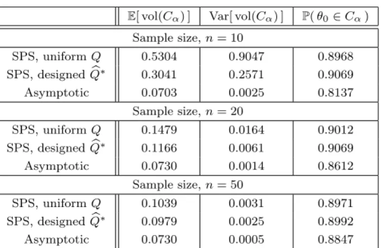
Table 1 contains the aggregated results of 3000 indepen- dent experiments for various confidence region construc- tions and sample sizes. As it was discussed in Section 3, we excluded the cases when the region was the whole space, thus, the expectations and variances are understood conditionally that the regions are non-degenerate.

We constrained X to matrices with tr(X^TX) ≤ 2. This constraint is QR decoupled and the D-optimal choice for R isR=I2, which we used forallconstructions. For SPS with input design we obtainedQusing the approximation algorithm outlined in Section 3.4 withKG= 250 and using 1000 randomly initialized local optimizations.

As the maximum allowed energy of the input signal was the same in each experiment, namely tr(X^TX) ≤ 2, independently of the sample size, the regions do not shrink as the sample size increases, and are directly comparable.

Note that SPS, both with and without input design, provides exact confidence regions, hence, the first two lines of the P(θ0 ∈ Cα) column for each sample size are around the desired 0.9. On the other hand, the classical confidence regions based on the asymptotic Gaussianity of the (scaled) estimation error are not guaranteed rigorously

Table 1. Empirical coverage and volume statis- tics (conditioned on non-degenerate regions)

E[ vol(Cα) ] Var[ vol(Cα) ] P(θ0∈Cα) Sample size,n= 10

SPS, uniformQ 0.5304 0.9047 0.8968

SPS, designed^Qb^{∗ 0.3041 0.2571 0.9069}

Asymptotic 0.0703 0.0025 0.8137

Sample size,n= 20

SPS, uniformQ 0.1479 0.0164 0.9012

SPS, designed^Qb

∗ 0.1166 0.0061 0.9069

Asymptotic 0.0730 0.0014 0.8612

Sample size,n= 50

SPS, uniformQ 0.1039 0.0031 0.8971

SPS, designed^Qb

∗ 0.0979 0.0025 0.8992

Asymptotic 0.0730 0.0005 0.8847

and underestimate the real uncertainty of the parameters, resulting in lower than required empirical coverage values.

The expected volumes with designed inputs,Qb^∗, are signif- icantly smaller than the ones based on a uniformly chosen Q. The improvements are between 6% and 42%, even though in both cases the optimal choice for R is used.

Moreover, the variance of the regions are also decreased with designing Q. Though, the expected volumes of the asymptotically designed regions are the smallest, their confidence probabilities are not correct, as it was noted.

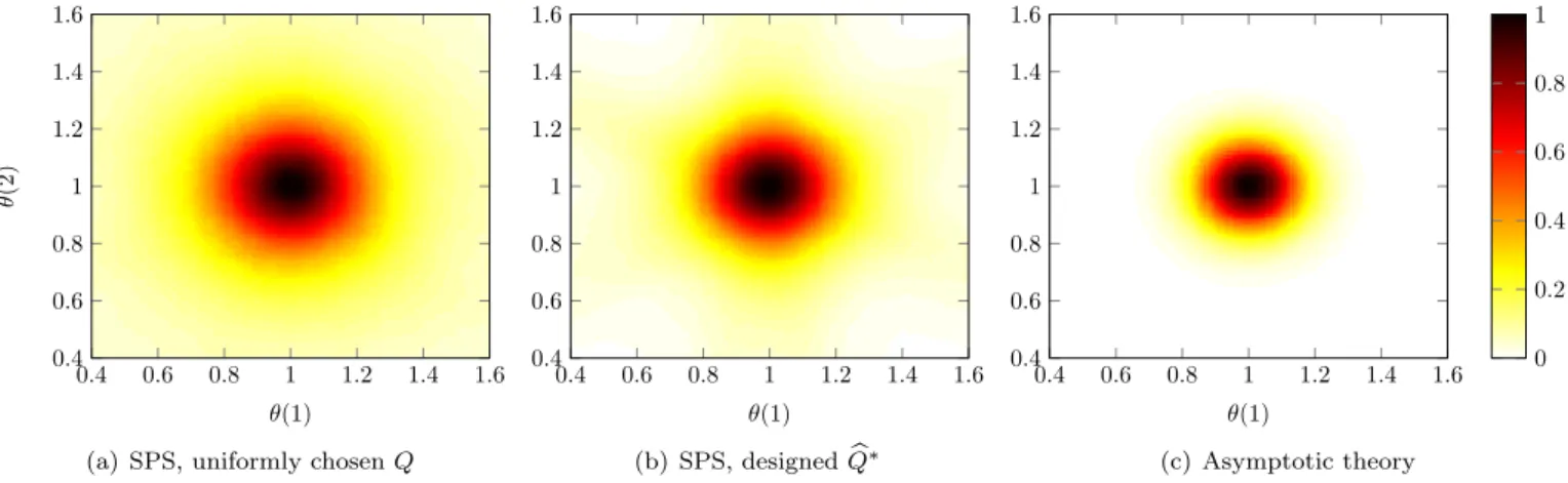
In order to give a more detailed view on the influence of in- put design on the shape of the confidence regions, Figure 1 shows the inclusion probability P(θ ∈ Cα) for different parameter values and confidence region constructions.

Figures 1(a) and 1(b) contain the heatmaps corresponding to SPS with uniformly random chosenQand designedQb^∗, respectively. The heatmap of the asymptotic confidence region is also given on Figure 1(c) for comparison.

5. CONCLUSIONS

Finite-sample system identification (FSID) aims at pro- viding methods with rigorous non-asymptotic guarantees under minimal statistical assumptions. Data-Perturbation (DP) methods generalize the Sign-Perturbed Sums (SPS) algorithm and can construct exact confidence regions using some mild distributional regularities of the noise.

In this paper we studied a natural input design problem for DP methods in which we aim at minimizing the expected volume of the confidence region. We explored the possibility of achieving this by individually minimizing the volumes of the fundamental building blocks of DP regions, namely, ellipsoids with confidence probability exactly¹/². It was shown that even handling such ellipsoids is hard in a finite sample setting, but can be achieved under certain decoupling assumptions, which also leads to nice connec- tions with the classical asymptotic theory. A Monte Carlo approximation was suggested to numerically solve the optimization and simulation experiments were presented indicating that minimizing the expected volumes of these fundamental ellipsoids carries over to the general case and reduces the expected sizes of DP confidence regions.

0.4 0.6 0.8 1 1.2 1.4 1.6 0.4

0.6 0.8 1 1.2 1.4 1.6

θ(1)

θ(2)

(a) SPS, uniformly chosenQ

0.4 0.6 0.8 1 1.2 1.4 1.6 0.4

0.6 0.8 1 1.2 1.4 1.6

θ(1) (b) SPS, designed^Qb

∗

0.4 0.6 0.8 1 1.2 1.4 1.6 0.4

0.6 0.8 1 1.2 1.4 1.6

θ(1)

0 0.2 0.4 0.6 0.8 1

(c) Asymptotic theory

Fig. 1. The probability of various parameter values,θ∈R², being included in the (random)C0.9 confidence region, for n = 10, depending on the method used to construct the region, and whether matrix Qis designed. Though the asymptotic theory provides the smallest regions, it underestimates the uncertainty of the parameters, cf. Table 1.

REFERENCES

Box, G.E.P. and Draper, N.R. (1987). Empirical Model- Building and Response Surfaces. John Wiley & Sons.

Car`e, A., Cs´aji, B.Cs., Campi, M., and Weyer, E. (2018).

Finite-sample system identification: An overview and a new correlation method.IEEE Control Systems Letters, 2(1), 61 – 66.

Cs´aji, B.Cs., Campi, M., and Weyer, E. (2012). Non- asymptotic confidence regions for the least-squares esti- mate. In Proceedings of the 16th IFAC Symposium on System Identification, 227 – 232.

Cs´aji, B.Cs., Campi, M., and Weyer, E. (2015). Sign- perturbed sums: A new system identification approach for constructing exact non-asymptotic confidence re- gions in linear regression models. IEEE Transactions on Signal Processing, 63(1), 169 – 181.

Garatti, S., Campi, M., and Bittanti, S. (2004). Assessing the quality of identified models through the asymptotic theory – when is the result reliable? Automatica, 40(8), 1319–1332.

Goodwin, G.C. and Payne, R.L. (1977). Dynamic System Identification: Experiment Design and Data Analysis.

Mathematics in Science and Engineering. Elsevier.

Kieffer, M. and Walter, E. (2014). Guaranteed charac- terization of exact non-asymptotic confidence regions as defined by LSCR and SPS. Automatica, 50, 507 – 512.

Kolumb´an, S. (2016).System Identification in Highly Non- Informative Environment. University Press.

Kolumb´an, S., Vajk, I., and Schoukens, J. (2015). Per- turbed datasets methods for hypothesis testing and structure of corresponding confidence sets. Automatica, 51, 326 – 331.

Ljung, L. (1999). System Identification - Theory for the User. Prentice Hall, 2nd edition.

Pintelon, R. and Schoukens, J. (2012). System Identi- fication: A Frequency Domain Approach. Wiley-IEEE Press, 2nd edition.

Rodrigues, M.I. and Iemma, A.F. (2014). Experimental Design and Process Optimization. CRC Press.

Weyer, E., Campi, M.C., and Cs´aji, B.Cs. (2017). Asymp- totic properties of SPS confidence regions. Automatica, 82, 287 – 294.

Appendix A. PROOF SKETCH FOR THEOREM 2 Here, the main steps of proving Theorem 2 are given without the detailed calculations. The first key ingredient is eq. (2.37) from Kolumb´an (2016) expressingZi(θ) as

Zi(θ) = (Y −Xθ0)^TG^TX[X^TX]⁻¹X^TG(Y −Xθ0) + + 2 (Y −Xθ0)^TG^TX[X^TX]⁻¹X^TGX(θ0−θ) + + (θ0−θ)^TX^TG^TX[X^TX]⁻¹X^TGX(θ0−θ).

This can be used to write Z0(θ)−Z1(θ) as a quadratic function of ∆ =θ0−θ. This quadratic function can be re- written into another form as a function of ∆+∆0for some

∆0, such that the linear term is eliminated (completing the square). The confidence regionC1/2 is the 0 level set of Z0(θ)−Z1(θ), so it corresponds to some non-zero level-set of the completed square. Performing some linear algebraic manipulations will lead to the statement of the theorem.

Appendix B. PROOF SKETCH FOR THEOREM 4 One of the main ingredients in proving Theorem 4 is the following lemma, that can be shown by simple algebraic manipulations and using the properties of projections.

Lemma 6. For anyQandG, andQe=T Q, whereT is an orthogonal matrix, we have that

Qe^TP^⊥

G^TQe

Qe=Q^TP_T^⊥TG^TT QQ. (B.1) We have already provided Lemma 5 which asserts thatQ1

and Q2 cannot be distinguished from each other if they can be transformed into one another by an element of the considered invariance groupG.

As we already mentioned in Section 3.2, every such pair of Q’s can be transformed into each other by an orthogonal matrix, so the last step is to show howQ1 andQ2can be compared ifQ1=T Q2holds only forT 6∈ G. We can define GT ,{G˜ ∈R^n×n :∃G∈ G: ˜G=T G}. The main obstacle in the proof is that the distribution of the noiseEappears in the comparison ofQ1 andQ2. By making a one to one correspondence between distributions invariant under G and those invariant underGT this can be bypassed and it follows that the comparison can be made solely based on the value ofQand the groupG, as given in Theorem 4.