D-optimal designs for complex Ornstein-Uhlenbeck processes

processes

S´ andor Baran

, Csilla Sz´ ak-Kocsis

and Milan Stehl´ık

1

Faculty of Informatics, University of Debrecen Kassai ´ ut 26, H-4028 Debrecen, Hungary

2

Department of Applied Statistics and Linz Institute of Technology, JKU Altenberger Straße 69, A-4040, Austria

3

Institute of Statistics, University of Valpara´ıso Gran Breta˜ na 1111, Valpara´ıso, Chile

Abstract

Complex Ornstein-Uhlenbeck (OU) processes have various applications in statistical modelling. They play role e.g. in the description of the motion of a charged test particle in a constant magnetic field or in the study of rotating waves in time-dependent reaction diffusion systems, whereas Kolmogorov used such a process to model the so-called Chandler wobble, small deviation in the Earth’s axis of rotation. In these applications parameter estimation and model fitting is based on discrete observations of the underlying stochastic process, however, the accuracy of the results strongly depend on the observation points.

This paper studies the properties of D-optimal designs for estimating the parameters of a complex OU process with a trend. We show that in contrast with the case of the classical real OU process, a D-optimal design exists not only for the trend parameter, but also for joint estimation of the covariance parameters, moreover, these optimal designs are equidistant.

Key words: Chandler wobble, complex Ornstein-Uhlenbeck process, D-optimality, op- timal design, parameter estimation.

1 Introduction

Random processes have various applications in statistical modelling in different areas of science such as physics, chemistry, biology or finance, where one usually cannot observe

1

continuous trajectories. In these situations parameter estimation and model fitting is based on discrete observations of the underlying stochastic process, however, the accuracy of the results strongly depend on the observation points. The theory of optimal experimental designs, dating back to the late 50s of the twentieth century (see e.g. Hoel, 1958; Kiefer, 1959), deals with finding design sets ξ={t₁, t₂, . . . , t_n} of distinct time points (or locations in space) where the process under study is observed, which are optimal according to some previously specified criterion (M¨uller, 2007). In parameter estimation problems the most popular criteria are based on the Fisher information matrix (FIM) of the observations. D-, E- and T-optimal designs maximize the determinant, the smallest eigenvalue and the trace of the FIM, respectively, an A-optimal design minimizes the trace of the inverse of the FIM (for an overview see Pukelsheim, 1993), whereas K-optimality refers to the minimization of the condition number of the FIM (see e.g. Ye and Zhou, 2013; Baran, 2017). In the last decades information based criteria have intensively been studied and despite the well developed theory for uncorrelated setup (see e.g. Silvey, 1980) only recently the more difficult correlated situation has been addressed (Dette et al., 2015, 2016).

In the present paper we derive D-optimal designs for parameter estimation of complex (or vector) Ornstein-Uhlenbeck (OU) processes with trend (see e.g. Arat´o, 1982), defined in detail in Section 2. A complex OU process describes e.g. the motion of a charged test particle in a constant magnetic field (Balescu, 1997), it is used in the description of the rotation of a planar polymer (Vakeroudis et al., 2011) or in the study of rotating waves in time-dependent reaction diffusion systems (Beyn and Lorenz, 2008; Otten, 2015), and it also has several applications in financial mathematics (see e.g. Barndorff-Nielsen and Shephard, 2001). Further, Kolmogorov proposed to model the so-called Chandler wobble, small deviation in the Earth’s axis of rotation (Lambeck, 1980), by the model

Z(t) =Z₁(t) +iZ₂(t) = me^i2πt+Y(t), t >0, (1.1) where Z₁(t) and Z₂(t) are the coordinates of the deviation of the instantaneous pole from the North Pole and Y(t) is a complex OU process (Arat´oet al., 1962).

We remark that the properties of D-optimal designs for classical one-dimensional OU processes have already investigated by Kiseˇl´ak and Stehl´ık (2008) and later by Zagoraiou and Baldi Antognini (2009), where the authors proved that there is no D-optimal design for estimating the covariance parameter, whereas the D-optimal design for trend estimation is equidistant and larger distances resulting in more information. Later these results were generalized for OU sheets under various sampling schemes (Baran and Stehl´ık, 2015; Baran et al., 2013, 2015).

2 Complex Ornstein-Uhlenbeck process with a trend

Consider the complex stochastic process Z(t) = Z1(t) +iZ2(t), defined as

Z(t) =mf(t) +Y(t), t≥0, (2.1)

with design points taken from the non-negative half-line R+, where m=m₁+im₂, m₁, m₂ ∈ R, f(t) = f₁(t) +if₂(t) with f₁(t), f₂(t) :R+7→R and Y(t) = Y₁(t) +iY₂(t), t≥0, is a complex valued stationary OU process. The process Y(t) can be defined by the stochastic differential equation (SDE)

dY(t) =−γY(t)dt+σdW(t), Y(0) =ξ, (2.2) where γ =λ−iω with λ >0, ω ∈R, σ > 0, W(t) = W₁(t) +iW₂(t), t≥0, is a standard complex Brownian motion, that is W₁(t) and W₂(t) are independent standard Brownian motions, and ξ =ξ1+iξ2, where ξ1 and ξ2 are centered normal random variables that are chosen according to stationarity (Arat´o, 1982).

Instead of the complex process Y(t) defined by (2.2) one can consider the two-dimensio- nal real valued stationary OU process Y1(t), Y2(t)>

defined by the SDE

"

dY₁(t) dY₂(t)

#

=A

"

Y₁(t) Y₂(t)

#

dt+σ

"

dW₁(t) dW₁(t)

#

, where A:=

"

−λ −ω

ω −λ

#

(2.3) We remark that in physics (2.3) is called A-Langevin equation, see e.g. (Balescu, 1997). If

Y₁(t), Y₂(t)>

satisfies (2.3) then Y₁(t) +iY₂(t) is a complex OU process which solves (2.2), and conversely, the real and imaginary parts of a complex OU process form a two- dimensional real OU process satisfying (2.3). Obviously, EY₁(t) = EY₂(t) = 0, whereas the covariance matrix function of the process Y1(t), Y2(t)>

is given by R(τ) :=E

"

Y₁(t+τ) Y₂(t+τ)

# "

Y₁(t) Y₂(t)

#^>

= σ²

2λe^Aτ = σ² 2λe^−λτ

"

cos(ωτ) −sin(ωτ) sin(ωτ) cos(ωτ)

#

, τ ≥0. (2.4) This results in a complex covariance function of the complex OU process Y(t) defined by (2.2) of the form

C(τ) :=EY(t+τ)Y(t) = σ²

λ e^−λτ cos(ωτ) +isin(ωτ)

, τ ≥0, behaving like a damped oscillation with frequency ω.

In the present study the damping parameter λ, frequency ω and standard deviation σ are assumed to be known. However, a valuable direction for future research will be the investigation of models where these parameters should also be estimated. Note that the estimation of σ can easily be done on the basis of a single realization of the complex process, see e.g. Arat´o (1982, Chapter 4). Now, without loss of generality, one can set the variances of Y₁(t) and Y₂(t) to be equal to one, that is σ²/(2λ) = 1, which reduces R(τ) to a correlation matrix function. Further results on the maximum-likelihood estimation of the covariance parameters can be found e.g. in Arat´o et al.(1999).

3 D-optimal designs

Suppose the complex process Z(t) is observed in design points 0 ≤ t1 < t2 < . . . < tn

resulting in the 2n-dimensional real vector Z₁(t₁), Z₂(t₁), Z₁(t₂), Z₂(t₂), . . . , Z₁(t_n), Z₂(t_n)^>

, where

Z₁(t) =m₁f₁(t)−m₂f₂(t) +Y₁(t), Z₂(t) =m₂f₁(t) +m₁f₂(t) +Y₂(t). (3.1) As it has mentioned in the Introduction, a D-optimal design maximizes the determinant of the FIM on the unknown parameters corresponding to the observations. Here we consider optimal designs for estimating the trend parameter m and the damping parameter λ and frequency ω, as well.

3.1 Estimation of the trend parameter

According to the results of e.g. Xia et al. (2006) or P´azman (2007) the FIM on parameter vector (m₁, m₂)^> based on observations

Z₁(t_j), Z₂(t_j)

, j = 1,2, . . . , n equals I_m1,m2(n) =H(n)C(n)⁻¹H(n)^>,

where

H(n) :=

"

f₁(t₁) f₂(t₁) f₁(t₂) f₂(t₂) · · · f₁(t_n) f₂(t_n)

−f₂(t₁) f₁(t₁) −f₂(t₂) f₁(t₂) · · · −f₂(t_n) f₁(t_n)

# ,

and C(n) is the 2n×2n covariance matrix of the observations.

Lemma 3.1 The FIM on trend parameters (m₁, m₂)^> of the two-dimensional analogue of the complex model (2.1) based on the real observation vector

Z₁(t_j), Z₂(t_j) , j = 1,2, . . . , n equals I_m1,m2(n) = Q(n)I2, where Ik, k ∈ N, denotes the k-dimensional unit matrix and

Q(n) := f₁²(t_n)+f₂²(t_n)+

n−1

X

j=1

1 1−e^−2λdj

f₁²(t_j) +f₂²(t_j) + e^−2λdj f₁²(t_j+1) +f₂²(t_j+1) (3.2) +2e^−λdj

f₁(t_j)f₂(t_j+1)−f₂(t_j)f₁(t_j+1)

sin(ωd_j)− f₁(t_j)f₁(t_j+1)+f₂(t_j)f₂(t_j+1)

cos(ωd_j) ,

with d_j :=t_j+1−t_j, j = 1,2, . . . , n−1.

Consider now the special case of a constant trend, that is the model

Z(t) = m+Y(t). (3.3)

In this situation f₁(t)≡1 and f₂(t)≡0, so

Z₁(t) =m₁+Y₁(t), Z₂(t) =m₂ +Y₂(t),

0 1 2 3 4 5

d₁

0 1 2 3 4 5

d2

(a) (b)

0 1 2 3 4 5

d₁

0 1 2 3 4 5

d2

(c) (d)

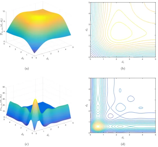
Figure 1: Bivariate objective function Dm1,m2 for a three-point design for (a) λ= 1, ω= 1 and (c) λ = 1, ω = 4, together with the corresponding contour plots (b) and (d), respectively.

and the expression in (3.2) reduces to Q(n) = 1+

n−1

X

`=1

g(d_`), where g(x) :=1−2e^−λxcos(ωx)+e^−2λx

1−e^−2λx , x >0, and g(0) := 0. (3.4) Hence, in order to obtain the D-optimal design, one has to find the maximum in d = (d₁, d₂, . . . , dn−1) of

D_m1,m2(d) := det I_m1,m2(n)

= 1 +

n−1

X

`=1

g(d_`)

!2

. (3.5)

Theorem 3.2 Consider the complex model (3.3) with ω 6= 0 observed in design points 0 ≤ t₁ < t₂ < . . . < t_n. The D-optimal design for estimating the trend parameter is

1 2 3 4 5 6 7 8 9 10 0

1 2 3 4

ω

d∗

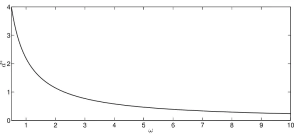
Figure 2: Location d^∗ of the global maximum of g(x) as a function of the frequency ω for λ= 1.

equidistant with d1 = d2 = . . . = dn−1 = d^∗, where d^∗ is the (existing) global maximum point of g(x).

Observe that for ω = 0 we have

Q(n) = 1 +

n−1

X

`=1

1−e^{−λd`</sup> 1 + e<sup>−λd`},

which is exactly the Fisher information on the constant trend parameter of a shifted real valued stationary OU process with covariance parameter λ (Kiseˇl´ak and Stehl´ık, 2008;

Zagoraiou and Baldi Antognini, 2009). In this case the D-optimal design on trend is also equidistant, however, with the increase of this equal distance the information is also increas- ing. According to the statement of Theorem 3.2 this is not the case for the complex OU process as there exists an optimal distance which provides the highest information.

Example 3.3 As an illustration consider a three-point design. Figures 1a and 1c show the bivariate objective function D_m1,m2 for λ = 1, ω = 1 and λ = 1, ω = 4 together with the corresponding contour plots (Figures 1b and 1d, respectively).

To get a better insight on the behavior of the optimal design, consider the function g(x) defined by (3.4). Figure 2 shows the location d^∗ of the global maximum of g(x) as a function of the frequency ω for λ = 1. The general case can obviously be obtained by rescaling both axes by the value of the damping parameter λ.

3.2 Estimation of the covariance parameters

Consider now the problem of estimating the damping parameter λ and frequency ω. Re- calling again the results of Xia et al. (2006) and P´azman (2007), the FIM on these parameters based on observations

Z₁(t_j), Z₂(t_j)

, j = 1,2, . . . , n has the form I_λ,ω(n) =

"

I_λ(n) I_λ,ω(n) I_λ,ω(n) I_ω(n)

#

, (3.6)

where

I_λ(n) := 1 2tr

C⁻¹(n)∂C(n)

∂λ C⁻¹(n)∂C(n)

∂λ

,

I_ω(n) := 1 2tr

C⁻¹(n)∂C(n)

∂ω C⁻¹(n)∂C(n)

∂ω

, (3.7)

I_λ,ω(n) := 1 2tr

C⁻¹(n)∂C(n)

∂λ C⁻¹(n)∂C(n)

∂ω

.

Note, that here I_λ(n) and I_ω(n) are Fisher information on parameters λ and ω, respectively, taking the other parameter as a nuisance.

Theorem 3.4 Consider the two-dimensional analogue of the complex model (3.3)with ω6=

0 observed in design points 0≤t₁ < t₂ < . . . < t_n. Then I_λ(n) =

n−1

X

`=1

ϕ(d_`), I_ω(n) =

n−1

X

`=1

ψ(d_`) and I_λ,ω(n) = 0, (3.8) where d_j =t_j+1−t_j, j = 1,2, . . . , n−1,

ϕ(x) :=x²e^−λxcosh(λx)

sinh²(λx) , ψ(x) := x²e^−λx

sinh(λx), x >0, and ϕ(0) := 1

λ², ψ(0) := 0. (3.9) Observe that none of the entries of the FIM I_λ,ω(n) depends on the frequency parameter.

Further, I_λ(n)/2 coincides with the Fisher information on the covariance parameter of a real valued OU process given by Zagoraiou and Baldi Antognini (2009). Note that here we consider two-dimensional OU processes, which justifies the halving of the information, however, due to this connection the first statement of the following theorem is a direct consequence of Zagoraiou and Baldi Antognini (2009, Theorem 4.2).

Theorem 3.5 Consider the two-dimensional analogue of the complex model (3.3)with ω6=

0 observed in design points 0≤t1 < t2 < . . . < tn.

a) The D-optimal design for the damping parameter λ maximizing the Fisher information I_λ(n) does not exist within the class of admissible designs.

0 1 2 3 4

d

0 0.02 0.04 0.06 0.08 0.1 0.12

Dm1,m2,λ,ω(d)

0 1 2 3 4

d

0 0.5 1 1.5 2 2.5 3

Dm1,m2,λ,ω(d)

(a) (b)

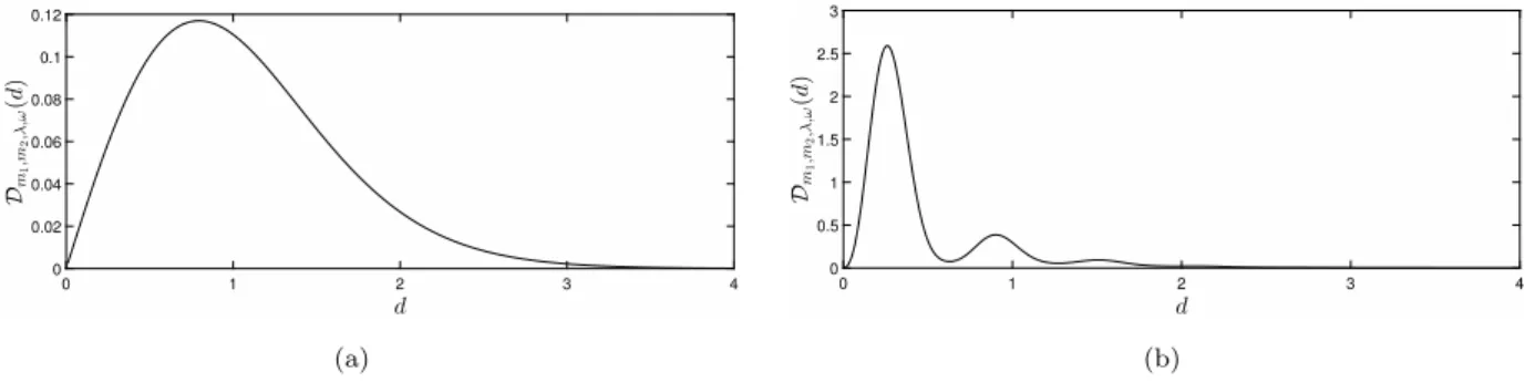
Figure 3: Objective function D_m1,m2,λ,ω for a two-point design for (a) λ= 1, ω = 1 and (b) λ= 1, ω = 4.

b) The D-optimal design for the frequency ω maximizing the Fisher information I_ω(n) is equidistant with

d₁ =d₂ =. . .=dn−1 =d_λ := 1 λ

W −2e⁻²

/2 + 1

≈ 0.7968

λ ,

where W(x) denotes the Lambert W-function (Corless et al., 1996).

c) The D-optimal design for both covariance parameters of the complex OU process max- imizing det I_λ,ω(n)

is equidistant with

d₁ =d₂ =. . .=dn−1 =d^◦/λ, where d^◦ ≈0.4930 is the unique positive solution of

1−d−2de^−2d−e^−4d = 0. (3.10)

We remark that in the case of one-dimensional OU processes an admissible design for the covariance parameter λ can be obtained by introducing the nugget effect, see e.g. Stehl´ık et al. (2017).

3.3 Estimation of all parameters

In the most general case one has to estimate both the components m₁, m₂ of the mean and the covariance parameters λ and ω. The FIM on these parameters equals

Im1,m2,λ,ω(n) =

"

Im1,m2(n) 02,2

0_2,2 I_λ,ω(n)

#

, (3.11)

where I_m1,m2(n) and I_λ,ω(n) are the information matrices defined in Lemma 3.1 and by (3.6), respectively, and 0<sub>k,`</sub> denotes the k ×` matrix of zeros. Hence, according to

0 1 2 3 4 5

d₁

0 1 2 3 4 5

d2

(a) (b)

0 1 2 3 4 5

d₁

0 1 2 3 4 5

d2

(c) (d)

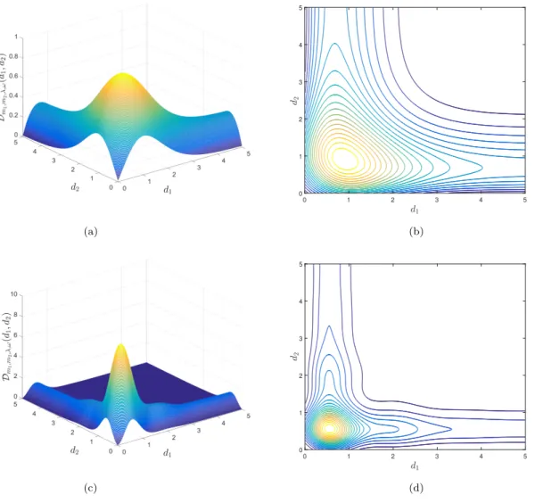
Figure 4: Bivariate objective function Dm1,m2,λ,ω for a three-point design for (a) λ = 1, ω = 1 and (c) λ = 1, ω = 4, together with the corresponding contour plots (b) and (d), respectively.

the results of Lemma 3.1 and Theorem 3.4, the D-optimal design for all four parameters maximizes in d= (d₁, d₂, . . . , dn−1)

D_m1,m2,λ,ω(d) := det I_m1,m2,λ,ω(n)

= 1 +

n−1

X

`=1

g(d_`)

!2 n−1

X

`=1

ϕ(d_`)

! _n−1 X

`=1

ψ(d_`)

!

, (3.12)

where the functions g, ϕ and ψ are defined by (3.4) and (3.9).

Example 3.6 Consider first the simplest case, that is a two-point design, when the objective function (3.12) is univariate. Figures 3a and 3b, showing the graph of D_m1,m2,λ,ω(d) for λ = 1, ω = 1 and λ = 1, ω = 4, respectively, clearly illustrate the existence of a finite optimal design.

0 1 2 3 4 5 6 7 8 9 10 0.2

0.4 0.6 0.8 1 1.2

ω

d∗

n=2 n=3 n=4 n=5 n=10 n=15 n=20

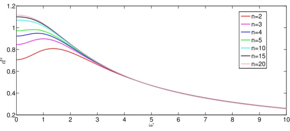
Figure 5: Optimal distance d^∗ of the equidistant n-point D-optimal design for estimation of all parameters as a function of the frequency ω for λ= 1.

Example 3.7 Similar to Example 3.3, consider again a three-point design. In Figures 4a and 4c the bivariate objective function D_m1,m2,λ,ω is plotted for λ = 1, ω = 1 and λ = 1, ω = 4, together with the corresponding contour plots (Figures 4b and 4d, respectively).

Although the objective function D_m1,m2,λ,ω(d) is too complicated for treating it analyt- ically, numerical results in higher dimensions show that there exists a D-optimal design and it is equidistant. In Figure 5 the optimal distance d^∗ of the equidistant n-point D-optimal design is plotted as a function of the frequency ω for λ = 1. Again, the general case can easily be obtained by rescaling both axes by the damping λ. Note that the larger the frequency, the smaller the effect of the number of design points on the optimal design.

4 Application

The application of the obtained designs, especially the ones given in Theorem 3.5 can be applied in the assessment of the quality of parameter estimation for damping parameter λ and frequency parameter ω in Kolmogorov’s model (1.1) of the Chandler wobble. The maximum likelihood estimator and sufficient statistics for λ are given in Arat´o (1968, 1982).

However, as noted after Theorem 3.5, for the drift parameter there exist no admissible design, unless we apply nugget effect.

For the model of Arat´o et al. (1962) two different estimates of the damping parameter are given by Panˇcenko (1960) (bλ= 0.3) and Walker and Young (1955) (bλ= 0.01). By the second statement of Theorem 3.5 the D-optimal design for frequency ω is equidistant with an optimal lag of d_λ ≈ ^0.7968_λ . However, the various estimates for λ give a broad range of optimal equidistant times for measurements.

0 0.5 1 1.5 2 2.5 3

λ

0 0.5 1 1.5 2 2.5 3

d

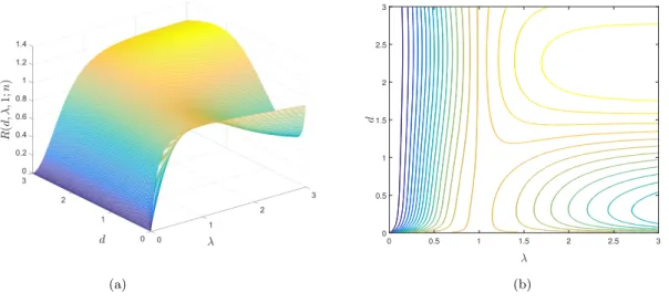
(a) (b)

Figure 6: Surface R(d, λ,1;n) (a) and the corresponding contour plot (b) for a ten-point equidistant design.

Further, due to the difference in the estimated values of the damping parameter λ, one might be interested in the sensitivity of the standardized setup (λ =ω = 1) with respect to the D-optimality criterion for estimation of the trend parameter. For then-point equidistant design this means the evaluation of R(d, λ,1;n), where

R(d, λ, ω;n) := 1+(n−1)g(d,1,1)2

1+(n−1)g(d, λ, ω)2, with g(x, λ, ω) :=1−2e^−λxcos(ωx)+e^−2λx

1−e^−2λx , (4.1) see also (3.4). Here we analyze the situation for arbitrary d, since experimenter usually does not have a free choice of the lag, although for λ = ω = 1 the optimal value equals d^∗ ≈ 2.1835 (see Theorem 3.2). Thus, this analysis incorporates all possible design spaces of form [0, T_max] where T_max denotes the upper bound of the design space.

The 3rd order Taylor expansion of R(d, λ,1;n) around the origin λ= 0 results in R(d, λ,1;n) =

d²

1 + (n−1)^(1−2e−d_1−e^cos(d)+e−2d ^−2d)

2

(n−1) cos(d)−12 λ²+O(λ³),

which shows a very high sensitivity of the efficiency for the standard design with respect to small values of the damping parameter λ. The same phenomenon can be observed on Figure 6 showing the surface R(d, λ,1;n) and the corresponding contour plot for a ten-point equidistant design.

If one can use the optimal lag d^∗ ≈2.1835 for the standard design (i.e. has the possibility of choosing an arbitrary lag), then the 3rd order Taylor expansion of R(d, λ,1;n) around the origin λ = 0 reduces to

R(d^∗, λ,1;n) = 1.9218· 1 + 1.1569·(n−1)2

(n−1)² λ²+O(λ³),

0 0.5 1 1.5 2 2.5 3

ω

0 0.5 1 1.5 2 2.5 3

d

(a) (b)

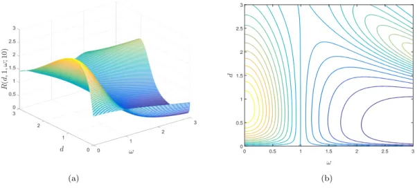
Figure 7: Surface R(d,1, ω;n) (a) and the corresponding contour plot (b) for a ten-point equidistant design.

that is for λ≈0 we have

n→∞lim R(d^∗, λ,1;n)≈2.5723λ².

This also confirms the sensitivity of the efficiency for the standard design at small damping values λ.

Consider now the sensitivity of efficiency for the standard design with respect to frequency ω. For the n-point equidistant design one has to evaluate R(d,1, ω;n) defined again by (4.1), which for ω≈0 indicates even higher sensitivity. This can be derived from the form

R(d,1, ω;n) = (n−2)e^−2d−2(n−1)e^−dcos(d) +n2

(n−2)e^−2d−2(n−1)e^−d+n2

− 2(n−1)d²e^−d (n−2)e^−2d−2(n−1)e^−dcos(d) +n2

(n−2)e^−2d−2(n−1)e^−d+n3 ω²+O(ω⁴).

of the 4th order Taylor expansion around ω = 0, and one can also observe it on Figure 7, where R(d,1, ω;n) and the corresponding contour plot are shown for a ten-point equidistant design.

Again, for the optimal lag d^∗ ≈2.1835 the 4th order Taylor expansion of R(d,1, ω;n) around the origin ω= 0 reduces to

R(d^∗,1, ω;n) = 2.0455(9.0024n−1.2211)² 6.2058n+ 1.5755−8.4655(n−1)ω²

(7.8777n+ 2)³ +O(ω⁴).

Hence, for ω ≈0 we have

n→∞lim R(d^∗,1, ω;n)≈1.9476−2.3318ω²,

which also confirms the sensitivity of the efficiency at small frequencies ω.

Recently Malkin and Miller (2010) discovered that besides the well-known Chandler wobble phase jump in the 1920s, two other large phase jumps have been identified in the 1850s and 2000s. As in the 1920s, these phase jumps occurred contemporary with a sharp decrease in the Chandler wobble amplitude. However, sharp decrease of amplitude can drastically change the optimal design, as confirmed by Theorem 3.5 for the case of a complex OU process. This underpins the importance of further research on stochastic approach to Chandler wobble. Moreover, substantial relation of large seismic events to Chandler wobble excitation (O’Connell and Dziewonski, 1976) justify further studies of optimal designs for both damping and frequency parameters.

Acknowledgements

This research was supported by the Hungarian – Austrian intergovernmental S&T coopera- tion program T´ET 15-1-2016-0046 and Project No. HU 11/2016. S´andor Baran is grateful for the support of the J´anos Bolyai Research Scholarship of the Hungarian Academy of Sci- ences. Milan Stehl´ık acknowledges the support of FONDECYT Regular Grant No 1151441.

A Appendix

A.1 Proof of Lemma 3.1

Similar to the real valued case (Zagoraiou and Baldi Antognini, 2009), the correlation matrix of observations

Z₁(t_j), Z₂(t_j)

, j = 1,2, . . . , n of the two-dimensional process (3.1) equals

C(n) =































I2 e^Ad1 e^A(d1+d2) e^A(d1+d2+d3) . . . e^{A(Pn−1j=1dj)} e^A>d1 I² e^Ad2 e^A(d2+d3) . . . e^{A(Pn−1j=2dj)} e^A>(d1+d2) e^A>d2 I2 e^Ad3 . . . e^{A(Pn−1j=3dj)} e^A>(d1+d2+d3) e^A>(d2+d3) e^A>d3 I2 . . . ...

... ... ... ... . .. ...

... ... ... ... . .. e^Adn−1

e^{A>(Pn−1j=1dj)} e^{A>(Pn−1j=2dj)} e^{A>(Pn−1j=3dj)} . . . e^A>dn−1 I²





























 .

Short calculation shows that the inverse of C(n) is given by

C⁻¹(n) =































U₁ −e^Ad1U₁ 0 0 . . . 0

−e^A>d1U₁ V₂ −e^Ad2U₂ 0 . . . 0 0 −e^A>d2U₂ V₃ −e^Ad3U₃ . . . 0

0 0 −e^A>d3U₃ V₄ . . . ...

... ... ... ... . .. ...

... ... ... ... V_n−1 −e^Adn−1U_n−1

0 0 0 . . . −e^A>dn−1Un−1 Un−1





























 ,

where U_k :=

I2 −e^(A+A>)dk−1

, k = 1,2, . . . , n−1, and V_k :=U_k+ e^(A+A>)dk−1Uk−1, k= 2,3, . . . , n−1, which is a direct generalization of the result of Kiseˇl´ak and Stehl´ık (2008) for the classical OU process.

Now, using (2.4) one can easily obtain

U_k= 1

1−e^−2λdkI2, e^AdkU_k = e^−λdk 1−e^−2λdk

"

cos(ωd_k) −sin(ωd_k) sin(ωd_k) cos(ωd_k)

#

, k= 1,2, . . . , n−1, V_k=

1

1−e^−2λdk + e^−2λdk−1 1−e^−2λdk−1

I2, k= 2,3, . . . , n−1,

which together with (2.4) specify both C(n) and C⁻¹(n). Finally, tedious but straightfor-

ward calculations lead us to (3.2).

A.2 Proof of Theorem 3.2

Consider first the function g(x) defined by (3.4). As g⁰(x) = r(x)

sinh²(λx) with r(x) := λcosh(λx) cos(ωx)+ωsinh(λx) sin(ωx)−λ, x >0, (A.1) the critical points of g(x) are the roots of r(x). Short calculation shows that r(x)<0 if and only if

λ

tanhλx 2

cotωx 2

2

+ 2ω

tanhλx 2

cotωx 2

−λ <0, (A.2) and the quadratic polynomial in (A.2) has two distinct roots

%−:= −ω−√

ω² +λ²

λ <0 and %₊ := −ω+√

ω²+λ²

λ >0.

Now, if ω 6= 0, by the properties of the cotangent and hyperbolic tangent functions there exist points

x⁻_n, n∈N such that 0< x⁻_n < x⁻_n+1 and

%− <tanhλx⁻_n 2

cotωx⁻_n 2

< %₊, that is r x⁻_n

<0, n ∈N.

Similar arguments prove the existence of points

x⁺_n, n ∈ N satisfying 0 < x⁺_n < x⁺_n+1 and r x⁺_n

>0, n ∈N. Thus, r(x) (and g⁰(x)) has an infinite number of sign changes, moreover, since limx→0g⁰(x) = ^ω_2λ² + ^λ₂ > 0, the first change is from positive to negative.

Denote by

x^◦_n, n∈N the roots of r(x), that is the critical points of g(x), where again, 0< x^◦_n< x^◦_n+1, n∈N, and x^◦₁ is a local maximum of g(x). Further, we have

g⁰⁰ x^◦_n

= λ²+ω²)cos ωx^◦_n sinh λx^◦_n. Assume that g⁰⁰ x^◦_n

= 0, that is ωx^◦_n = ^π₂ +πkn for some kn∈Z. In this case 0 = r x^◦_n

=±ωsinh λ

ω π

2 +πk_n

−λ, (A.3)

where the positive sign will apply if k_n is odd, and the negative sign if it is even. However, the Taylor series expansion of the hyperbolic sine implies

±ωsinh λ

ω π

2 +πk_n

−λ =±λπ

2 ∓1 +πk_n

±

∞

X

`=1

λ<sup>2`+1</sup> (2`+ 1)!ω^2`

π

2 +πk_n2`+1

6= 0,

which contradicts to (A.3). Hence, for the critical points

x^◦_n, n ∈ N of g(x) either g⁰⁰ x^◦_n

<0 or g⁰⁰ x^◦_n

>0, so they are either local maxima or local minima, respectively.

This ensures the existence of a global maximum of g as well at some point d^∗ ∈

x^◦_n, n∈N , where g⁰(d^∗) = 0, and g⁰⁰(d^∗)<0.

Obviously, instead of D_m1,m2 defined by (3.5) it suffices to maximize F(d₁, d₂, . . . , dn−1) :=Q(n) = 1 +

n−1

X

`=1

g d_`

Now, consider the (n−1)-dimensional vector d^∗ := (d^∗, d^∗, . . . , d^∗)^>. As

∂F

∂d_k(d^∗, d^∗, . . . , d^∗) = g⁰(d^∗) = 0, k = 1,2, . . . , n−1, d^∗ is a critical point of F. Further, as

∂²F

∂d<sub>`</sub>∂d<sub>k</sub>(d<sup>∗</sup>, d<sup>∗</sup>, . . . , d<sup>∗</sup>) = 0 if k6=`, k, `= 1,2, . . . , n−1, and

∂²F

∂d²_k(d^∗, d^∗, . . . , d^∗) =g⁰⁰(d^∗)<0, k = 1,2, . . . , n−1,

the Hessian of F at d^∗ is negative definite. Hence, d^∗ is a maximum point of F and since the components g(d^∗) are the largest possible, this maximum is global.

A.3 Proof of Theorem 3.4

Using the expressions of the covariance matrix C(n) of observations and its inverse C⁻¹(n) given in the proof of Lemma 3.1 and (3.6), the formulae of (3.8) can be verified by induction, similar to the proof of Theorem 2 of Baran and Stehl´ık (2015). As an example consider the Fisher information on damping parameter λ, where one has to show

I_λ(n) := 1 2tr

C⁻¹(n)∂C(n)

∂λ C⁻¹(n)∂C(n)

∂λ

=

n−1

X

`=1

2d²_{`</sub>q<sub>`}²(1 +q_`²)

(1−q_`²)² , (A.4) with q_k := e^−λdk, k= 1,2, . . . , n−1.

For n = 2 equation (A.4) holds trivially. Assume also that (A.4) is true for some n, and we are going to show it for n+ 1. Let

∆(n) := −(d₁+d₂+. . .+d_n)q₁q₂. . . q_nB_1,...,n,−(d₂+d₃. . .+d_n)q₂q₃. . . q_nB_2,...,n, . . . ,−d_nq_nB_n>

,

where

B_k,...,n :=

"

cos ω(d_k+. . .+d_n)

−sin w(d_k+. . .+d_n) sin ω(d_k+. . .+d_n)

cos ω(d_k+. . .+d_n)

#

, k= 1,2, . . . , n.

Using the representations of C(n) and C⁻¹(n) given in Section A.1, one can easily see

∂C(n+1)

∂λ =





∂C(n)

∂λ ∆(n)

∆^>(n) 0_2,2



 and C⁻¹(n+1) =

"

C⁻¹(n) Λ_1,2(n) Λ^>_1,2(n) (1−q_n²)⁻¹I2

# +

"

Λ1,1(n) 02n,2

0_2,2n 0_2,2

# ,

where 0<sub>k,`</sub> denotes the k×` matrix of zeros and Λ_1,1(n) :=







02n−2,2n−2 02n−2,2

02,2n−2

q_n² 1−q_n²I2





 and Λ_1,2(n) :=





02n−2,2

− q_n 1−q_n²B_n



.

In this way

C⁻¹(n+ 1)∂C(n+ 1)

∂λ =











C⁻¹(n)∂C(n)

∂λ +K_1,1(n) C⁻¹(n)∆(n) K_1,2(n) d_nq_n²

1−q_n²I²









 +

"

K2,1(n) K2,2(n) 0_2,2n 0_2,2

# ,

with K_1,1(n) :=





02n−2,2n

− q_n

1−q²_nB_n∆^>(n)



, K_1,2(n) := 1

1−q²_n∆^>(n)− q_n 1−q_n²B_n^>h

∆^>(n−1) 0_2,2 i

,

K_2,1(n) :=







02n−2,2n−2 02n−2,2

q_n²

1−q²_n∆^>(n−1) 0_2,2





, K_2,2(n) :=







02n−2,2

− d_nq_n³ 1−q²_nB_n





.

Hence,

I_λ(n+1) =I_λ(n) + tr

C⁻¹(n)∂C(n)

∂λ K_1,1(n)

+ tr

C⁻¹(n)∆(n)K_1,2(n) +1 2tr

K²_1,1(n) + d²_nq_n⁴

(1−q_n²)² + tr

C⁻¹(n)∂C(n)

∂α K_2,1(n)

+ tr

K_1,2(n)K_2,2(n) . (A.5) After long but straightforward calculations one can get

tr

C⁻¹(n)∂C(n)

∂λ K_1,1(n)

= −

n−1

X

`=1

2d²_{`</sub>q<sub>`}²q_`+1² ·. . .·q_n²

(1−q_`²)(1−q_n²) =−tr

C⁻¹(n)∂C(n)

∂λ K_2,1(n)

,

tr

C⁻¹(n)∆(n)K1,2(n) = 2d²_nq²_n

(1−q_n²)² − 2d²_nq⁴_n (1−q_n²)², 1

2tr

K²_1,1(n) = d²_nq_n⁴

(1−q_n²)², tr{K_1,2(n)K_2,2(n)}= 2d²_nq⁴_n (1−q_n²)², so (A.5) implies

I_λ(n+ 1) =I_λ(n) + 2d²_nq_n²(1 +q_n²) (1−q_n²)² ,

which completes the proof of (A.4). The other two statements of Theorem 3.4 can be verified

in a similar way.

A.4 Proof of Theorem 3.5

As it has been mentioned, statement a) directly follows from Theorem 4.2 of Zagoraiou and Baldi Antognini (2009).

Now, consider the function ψ(x) defined by (3.8). As ψ⁰(x) = 4xe^−2λx 1−λx−e^−2λx

1−e^−2λx2 , ψ(x) has a single critical point at d^∗ := _λ¹ W(−2e⁻²)/2 + 1

, moreover, ψ⁰⁰(d^∗)<0, so d^∗ is a global maximum point. Hence, statement b) can be verified using the same arguments as in the proof of Theorem 3.2.

According to (3.8), the D-optimal design on λ and ω maximizes G(d₁, d₂, . . . , dn−1) :=

n−1

X

`=1

ϕ(d_`)

! _n−1 X

`=1

ψ(d_`)

!

=

n−1

X

`=1

2d<sub>`</sub><sup>2</sup>e<sup>−2λd`</sup> 1 + e^{−2λd`</sup> 1−e<sup>−2λd`}2

! _n−1 X

`=1

2d<sub>`</sub><sup>2</sup>e<sup>−2λd`</sup> 1−e^−2λd`

! ,

and obviously, it suffices to consider the case λ= 1. The critical points of G are solutions of the system

∂G

∂d_k(d₁, d₂, . . . , dn−1) =ϕ⁰(d_k)

n−1

X

`=1

ψ(d_`)

!

+ψ⁰(d_k)

n−1

X

`=1

ϕ(d_`)

!

= 0, (A.6) k = 1,2, . . . , n−1, where

ϕ⁰(x) = 4xe^−2λx 1−λx−3λxe^−2λx−e^−4λx

1−e^−2λx3 <0, x >0.

Hence, for λ= 1 the system of equations (A.6) is equivalent to κ(d_k) =

n−1

X

`=1

ψ(d_`)

! ⁿ⁻¹ X

`=1

ϕ(d_`)

!

, k = 1,2, . . . , n−1, (A.7) where

κ(x) := 1−x+ (x−2)e^−2x+ e^−4x

x−1 + 3xe^−2x+ e^−4x , x >0.

Since κ(x) is strictly monotone decreasing and continuous with limx→0κ(x) = 1 and limx→∞κ(x) = −1, the solution of (A.7) should satisfy d₁ =d₂ =. . .=dn−1 =:d. Hence, the critical points of G have equal coordinates and at a critical point (A.7) reduces to κ(d) = 1−e^−2d

/ 1 + e^−2d

, which is equivalent to (3.10). The latter equation has a unique positive solution d^◦, so d1 =d2 =. . .=dn−1 =d^◦ is the only critical point of G.

Short calculation shows that at this point the Hessian of G equals H = (n−1)

ϕ⁰⁰(d^◦)ψ(d^◦) +ψ⁰⁰(d^◦)ϕ(d^◦)

Iⁿ⁻¹+ 2

ϕ⁰(d^◦)ψ⁰(d^◦)

1n−11^>_n−1

≈ −0.5083·(n−1)Iⁿ⁻¹−0.2754·1n−11^>_n−1,

where 1_k, k ∈ N, denotes the k-dimensional vector of ones. This means that for all 0 6=v = (v₁, v₂, . . . , vn−1)^>∈Rⁿ⁻¹ we have

v^>Hv = (n−1)

ϕ⁰⁰(d^◦)ψ(d^◦) +ψ⁰⁰(d^◦)ϕ(d^◦)

v^>v+ 2

ϕ⁰(d^◦)ψ⁰(d^◦)

n−1

X

`=1

v`

!2

<0, so the Hessian is negative definite. Hence, the unique critical point of G is a global

maximum, which completes the proof.

References

Arat´o, M. (1968) Confidence limits for the parameter λ of a complex stationary Gaussian- Markovian process. Theory Probab. Appl. 13, 314–320.

Arat´o, M. (1982) Linear Stochastic Systems with Constant Coefficients. A Statistical Ap- proach. Springer, Berlin (in Russian: Nauka, Moscow, 1989).

Arat´o, M., Baran, S. and Isp´any, M. (1999) Functionals of complex Ornstein-Uhlenbeck processes. Comput. Math. Appl.37, 1–13.

Arat´o, M., Kolmogorov, A. N. and Sinay, Yu. G. (1962) Estimation of the parameters of a complex stationary Gaussian Markov process. Dokl. Akad. Nauk. SSSR 146, 747–750.

Balescu, R. (1997)Statistical Dynamics – Matter out of Equilibrium.Imperial College Press, London.

Baran, S. (2017) K-optimal designs for parameters of shifted Ornstein-Uhlenbeck processes and sheets. J. Stat. Plan. Inference 186, 28–41.

Baran, S., Sikolya, K. and Stehl´ık, M. (2013) On the optimal designs for prediction of Ornstein-Uhlenbeck sheets.Statist. Probab. Lett. 83, 1580–1587.

Baran, S., Sikolya, K. and Stehl´ık, M. (2015) Optimal designs for the methane flux in troposphere. Chemometr. Intell. Lab. 146, 407–417.

Baran, S. and Stehl´ık, M. (2015) Optimal designs for parameters of shifted OrnsteinUhlen- beck sheets measured on monotonic sets. Statist. Probab. Lett. 99, 114–124.

Barndorff-Nielsen, O. R. and Shephard, N. (2001) Non-Gaussian Ornstein-Uhlenbeck-based models and some of their uses in financial economics. J. R. Statist. Soc. B 63, 167–241.

Bayn, W. J.and Lorenz, J. (2008) Nonlinear stability of rotating patterns. Dyn. Partial Differ. Equ. 5, 349–400.

Corless, R. M., Gonnet, G. H., Hare, D. E. G., Jeffrey, D. J. and Knuth, D. E. (1996) On the Lambert W function. Adv. Comput. Math. 5, 329–359.

Dette, H., Pepelyshev, A. and Zhigljavsky, A. (2015) Design for linear regression models with correlated errors. In: Dean, A., Morris, M., Stufken, J. and Bingham, D. (eds.),Handbook of Design and Analysis of Experiments.Chapman & Hall/CRC, Boca Raton, pp. 237–278.

Dette, H., Pepelyshev, A. and Zhigljavsky, A. (2016) Optimal designs in regression with correlated errors. Ann. Statist. 44, 113–152.

Hoel, P. G. (1958). Efficiency problems in polynomial estimation. Ann. Math. Stat. 29, 1134–1145.

Kiefer, J. (1959) Optimum experimental designs (with discussions). J. R. Statist. Soc. B 21, 272–319.

Kiseˇl´ak, J. and Stehl´ık, M. (2008) Equidistant D-optimal designs for parameters of Ornstein- Uhlenbeck process.Statist. Probab. Lett. 78, 1388–1396.

Lambeck, K. (1980) The Earth’s Variable Rotation: Geophysical Causes and Consequences.

Cambridge University Press, Cambridge.

Malkin, Z. and Miller, N. (2010) Chandler wobble: two more large phase jumps revealed.

Earth Planets Space 62, 943–947.

M¨uller, W. G. (2007)Collecting Spatial Data. Third Edition. Springer, Heidelberg.

O’Connell, R. J. and Dziewonski, A. M. (1976) Excitation of the Chandler wobble by large earthquakes. Nature 262, 259–262.

Otten, D. (2015) Exponentially weighted resolvent estimates for complex Ornstein-Uhlen- beck systems. J. Evol. Eq. 15, 753–799.

Panˇcenko, N. I. (1960) On the question of the decay of free nutation. Proc. 14th Astronom.

Conf. USSR Izdat. Akad. Nauk SSSR, Moscow, pp. 232–243 (in Russian).

P´azman, A. (2007) Criteria for optimal design of small-sample experiments with correlated observations. Kybernetika 43, 453–462.

Pukelsheim, F. (1993) Optimal Design of Experiments. Wiley, New York.

Silvey, S. D. (1980) Optimal Design. Chapman & Hall, London.

Stehl´ık, M., Helpersdorfer, Ch., Hermann, P., Supina, J., Grilo, L. M., Maidana, J. P., Fuders, F. and Stehlikova, S. (2017) Financial and risk modelling with semicontinuous covariances. Inform. Sciences 394–395, 246–272.

Vakeroudis, S., Yor, M. and Holcman, D. (2011) The mean first rotation time of a planar polymer. J. Stat. Phys. 143, 1074–1095.

Walker, A. M. and Young, A. (1955) The analysis of the observations of the variation of the lattitude. Monthly Notices Roy. Astronom. Soc. 115, 443–459.

Xia, G., Miranda, M. L. and Gelfand, A. E. (2006) Approximately optimal spatial design approaches for environmental health data. Environmetrics 17, 363–385.

Ye, J. and Zhou, J. (2013) Minimizing the condition number to construct design points for polynomial regression models. Siam. J. Optim. 23, 666–686.

Zagoraiou, M. and Baldi Antognini, A. (2009) Optimal designs for parameter estimation of the Ornstein-Uhlenbeck process. Appl. Stoch. Models Bus. Ind. 25, 583–600.