On Optimistic and Pessimistic Bilevel Optimization Models for Demand Response Management

Article

On Optimistic and Pessimistic Bilevel Optimization Models for Demand Response Management

Tamás Kis, András Kovács * and Csaba Mészáros

Citation: Kis, T.; Kovács, A.;

Mészáros, C. On Optimistic and Pessimistic Bilevel Optimization Models for Demand Response Management.Energies2021,14, 2095.

https://doi.org/10.3390/en14082095

Academic Editors: Miadreza Shafie-khah and Mohammad Ali Fotouhi Ghazvini

Received: 14 March 2021 Accepted: 2 April 2021 Published: 9 April 2021

Publisher’s Note:MDPI stays neutral with regard to jurisdictional claims in published maps and institutional affil- iations.

Copyright: © 2021 by the authors.

Licensee MDPI, Basel, Switzerland.

This article is an open access article distributed under the terms and conditions of the Creative Commons Attribution (CC BY) license (https://

creativecommons.org/licenses/by/

4.0/).

EPIC Center of Excellence in Production Informatics and Control, Institute for Computer Science and Control (SZTAKI), Eötvös Loránd Research Network (ELKH), Kende u. 13-17, 1111 Budapest, Hungary;

tamas.kis@sztaki.hu (T.K.); csaba.meszaros@sztaki.hu (C.M.)

* Correspondence: akovacs@sztaki.hu

Abstract:This paper investigates bilevel optimization models for demand response management, and highlights the often overlooked consequences of a common modeling assumption in the field.

That is, the overwhelming majority of existing research deals with the so-called optimistic variant of the problem where, in case of multiple optimal consumption schedules for a consumer (follower), the consumer chooses an optimal schedule that is the most favorable for the electricity retailer (leader).

However, this assumption is usually illegitimate in practice; as a result, consumers may easily deviate from their expected behavior during realization, and the retailer suffers significant losses. One way out is to solve the pessimistic variant instead, where the retailer prepares for the least favorable optimal responses from the consumers. The main contribution of the paper is an exact procedure for solving the pessimistic variant of the problem. First, key properties of optimal solutions are formally proven and efficiently solvable special cases are identified. Then, a detailed investigation of the optimistic and pessimistic variants of the problem is presented. It is demonstrated that the set of optimal consumption schedules typically contains various responses that are equal for the follower, but bring radically different profits for the leader. The main procedure for solving the pessimistic variant reduces the problem to solving the optimistic variant with slightly perturbed problem data.

A numerical case study shows that the optimistic solution may perform poorly in practice, while the pessimistic solution gives very close to the highest profit that can be achieved theoretically. To the best of the authors’ knowledge, this paper is the first to propose an exact solution approach for the pessimistic variant of the problem.

Keywords:demand response; bilevel optimization; pessimistic case; polynomial time algorithm

1. Introduction

Stackelberg game models and the corresponding bilevel programming solution ap- proaches for demand response management have received considerable attention recently.

When focusing on the operational level, most models capture the interplay of an electricity retailer, who is the leader in the Stackelberg game, and its multiple consumers, who act as the followers. In the sequential game, the leader decides first on the electricity tariff or some other incentives, whereas the followers respond to the tariff by scheduling their loads accordingly. Stackelberg game models assume that the load response is calculated by solving an optimization problem, with the tariff as the parameter, to optimality. Numerous such approaches have been published, including models with deferrable or curtailable loads, batteries, electric vehicles (EVs), etc. [1–5].

In this paper, it is argued that despite the remarkable results, an important detail is frequently overlooked: the followers often have a large set of optimal solutions to their problems, and the selection of the response from this set is not defined properly. Moreover, different optimal solutions for the follower may bring radically different benefits for the leader. In bilevel optimization, the optimistic assumption states that the followers select

Energies2021,14, 2095. https://doi.org/10.3390/en14082095 https://www.mdpi.com/journal/energies

their optimal solution that is the most favorable for the leader. In contrast, the pessimistic variant deals with the case where the followers return their least favorable optimal response to the leader, and hence, it safeguards from potential losses due to an unexpected selection.

Most previous approaches in the literature implicitly make the optimistic assumption, although this assumption can hardly be enforced in practice. In this paper, the difference between the two variants of the bilevel problem is highlighted. Then, to the best of the authors’ knowledge, the first efficient exact solution approach for the pessimistic variant of a bilevel electricity tariff optimization problem in the literature is introduced. Moreover, it is shown that in most cases, the profit of the leader in the pessimistic variant can approach the profit that can be achieved in the optimistic variant.

It is important to emphasize at this point the difference between bilevel optimization as a mathematical modeling and solution approach, and hierarchical modeling techniques in general. Bilevel optimization [6] applies formal mathematical techniques to characterize and find the equilibrium in game-theoretical decision situations with two fully rational parties with given constraints and objectives, and a well-defined serial decision workflow.

This is different from generic hierarchical modeling techniques that analyze the interplay of two or more decision makers, typically by solving the problems faced by the individual parties one by one, and constructing the overall outcome by assuming some coordination mechanism between them, often using simulation techniques; see, e.g., [7]. This paper considers bilevel optimization strictly in the former sense.

Main results. On the one hand, this paper proves formal properties of the optimal solutions of a bilevel tariff optimization problem, both for the easily tractable single- consumer special case, and the computationally hard general case with an arbitrary number of consumers. The main implication of these results is the reduction of the pessimistic variant to the optimistic one by perturbing the problem data and also the optimal price vector, which also results in the first efficient solution approach for the pessimistic variant.

On the other hand, a numerical case study is presented that demonstrates that solving the optimistic problem may directly cause a significant loss of profit for the retailer if the consumers do not choose their optimal solution as expected.

Structure of the paper.After a brief literature review in Section2, the bilevel electricity tariff optimization problem is defined formally in Section3. Some general observations are presented in Section4. In Section5, a special case with one consumer only is studied. The general optimistic variant is treated in Section6.1, and the pessimistic one in Section6.2. An experimental evaluation is presented in Section7, and the paper concludes in Section8.

2. Literature Review

Introduced by the seminal paper of Bracken and McGill [8], bilevel optimization has become a field rich in deep theoretical results and with many practical applications; see, e.g., Bard [9], Dempe [6], and Colson et al. [10]. One of the central questions is expressing the optimality of the followers’ solutions in mathematical programming formulations. To this end, Karush–Kuhn–Tucker (KKT) necessary optimality conditions, or the Fritz John necessary optimality conditions, value functions, or penalty functions can be used [11–16].

As for the methods, the optimistic or strong bilevel optimization problem appears to be easier to solve than the pessimistic or weak bilevel problem in general; see, e.g., [17].

Most approaches reduce the strong bilevel optimization problem to a single-level problem by expressing the optimality of the lower-level solution by using one of the techniques mentioned above and then applying some non-linear programming methods for solving the resulting formulation [18]. There are many results for special cases. The linear bilevel programming problem, in which all constraints and objective functions are linear, is well understood; see, e.g., Ben-Ayed [19] and Dempe [6]. Lozano and Smith [20] described an exact method for nonlinear bilevel optimization problems, in which the leader has only integer variables, while the follower can have both integer and continuous variables.

The constraints and the objective functions can be nonlinear, but all constraints are separa- ble in terms of the leader and follower variables. They used a value function-based problem

formulation in their enumeration procedure, and they extended it to the pessimistic prob- lem as well. Since the leader’s variables can take only discrete values, an optimal solution always exists, provided the problem is feasible. Brotcorne et al. [21] studied a concrete application in which the leader sets freight tariffs on the arcs of a traffic network, and the follower aims at minimizing its transportation costs while satisfying transportation de- mands. Both objective functions are non-linear, but all constraints are linear. The authors proposed heuristics to obtain good solutions.

As for the weak variant, Loridan and Morgan [22], approximated the optimal solution by solving a sequence of strong bilevel optimization problems. Wiesemann et al. [23]

provided an in-depth study of the pessimistic bilevel optimization problem under some restrictions. That is, the follower’s feasible set must be independent of the leader’s solu- tion, and both the leader and the follower must have a compact set of feasible solutions.

However, integrality of the variables at both levels is permitted. Under these assumptions, the optimal solution is approximated by solving a sequence of problems obtained by relax- ing the value function of the follower by a decreasing sequence of additive constants. A new relaxation, based on the value function approach, was proposed by Zeng [17]. The ap- proach works if an optimal solution exists, but the author also discussed some remedies when that is not the case, which may help sometimes. The crux of the method is to reduce the pessimistic bilevel optimization problem to solving one or two optimistic problems with a few additional constraints.

The electricity tariff optimization problem in scope and its various extensions have been investigated extensively in the electrical engineering community for demand response management in smart grids. This formulation is named the simple multi-period energy tariff optimization problem (SMETOP) in [24], where its NP-hardness is proved in case of multiple followers. Various papers address the extensions of the SMETOP, including generic piecewise linear, quadratic, or other non-linear follower utility functions [3,4];

battery storage at the follower [2], multi-energy systems [25]; or the heating, ventilation, and air-conditioning (HVAC) of buildings using a dedicated thermal model [26]. The typical solution approach is reformulating the bilevel problem into an equivalent single-level problem using the KKT conditions, eliminating non-linear terms, and then solving the model as a mixed-integer linear program (MILP) [3,5,27,28]. The possible alternatives include exploiting strong duality for the follower’s linear problem to convert the problem into a single-level quadratic program [2], or to use custom (meta-)heuristics to keep the computational load at bay [4,29,30]. A more detailed review on the solution approaches to bilevel programming models of demand response management can be found, e.g., in [2].

However, these approaches are applicable only to the optimistic (strong) variant of the bilevel problem. Applications of bilevel programming to energy networks are reviewed in [18]. Extensions to the stochastic case are presented, e.g., in [31,32].

The difference between the optimistic and the pessimistic variants of the bilevel op- timization problem specifically in energy management is emphasized in [33]. The paper introduces the notion of a deceiving solution to denote the worst possible outcome for the leader if it applies the optimistic assumption but the follower deviates from the ex- pected response, and similarly, the rewarding solution for the best possible outcome if the leader applies the pessimistic assumption but the follower decides for an unexpectedly favorable response. The paper applies a hybrid solution approach by combining a genetic algorithm and a MILP solver to find close-to-optimal solutions for both the optimistic and the pessimistic variants of the semivectorial bilevel problem in which the follower addresses the minimization of the bi-criteria composed of electricity cost and discomfort.

However, the authors are not aware of efficient exact solution approaches to pessimistic bilevel optimization problems applicable to energy management.

3. Problem Definition

The paper investigates a bilevel electricity tariff optimization problem for demand response management as follows. In the bilevel problem, the leader is an electricity retailer

who controls the electricity tariff (unit price) over a finite time horizon divided intoTtime periods, e.g., the 24 hours of a day. For eacht∈ {1, . . . ,T}, letctbe the wholesale market price of electricity,Qthe average unit price, andq^l_tandq^u_t the lower and upper bounds, respectively, on the unit price of the electricity (to be determined by the leader) in time periodt. There aremfollowers, the consumers, who buy electricity at the given prices over the time horizon in order to meet their demands. Followeriattributes some utilityuit

to consuming one unit of electricity in each time periodt, its total demand over the time horizon is at leastD^l_i and at mostD^u_i, and its consumption will be betweenx^l_itandx^u_itin each time periodt.

It is noted that different loads of a household, which are scheduled independently (e.g., air conditioning, a washing machine, an EV charger, and other, inflexible loads) can be captured as separate consumers (followers) in the model. Likewise, a single consumer in the model can capture the ensemble of consumers with similar parameters in reality.

The profit of the leader, for a given price vectorq, and the consumption vectorxof the followers, are

p(q,x)_:=

∑

∑

(qt−ct)x_it.

The leader wants to determine the unit pricesqtin order to maximize its profit, that is,

MaximizeF(q) (1)

subject to the constraints 1 T

∑

qt≤Q (2)

q^l_t≤qt≤q^u_t, t=1, . . . ,T, (3) whereFis a function mapping the price vector to a profit value, and it can be evaluated after the followers solve their own optimization problems. Fis defined after presenting the followers’ optimization problems. In fact, each followerisolves a continuous knap- sack problem in which the objective function is parameterized by the price vector set by the leader:

Maximize

∑

(uit−qt)xit (4)

D^l_i ≤

∑

xit ≤D^u_i (5)

x^l_it ≤x_it ≤x_it^u, t=1, . . . ,T (6) Assuming that (5)–(6) has a solution, each followerihas at least one optimal solution for any price vectorq. Let Ω(q) ⊂ R^m×T denote the set of all optimal solutions of the followers. Observe thatΩ(q)is never empty. If the followers have a unique optimal solution forq, i.e.,Ω(q)contains only one element, then the leader’s profit is well defined forq. However, ifΩ(q)has 2 or more members, then it is not clear in advance, which optimal solution would be returned by the followers. For instance, ifuit−qt=u_it⁰−q_t⁰, x^u_it =x^u_it0, andx^l_it=x^l_it0, for somet6=t⁰, and eitherxitorxit⁰can be set to upper bound in an optimal solution, then it is up to followeriwhich one to choose. However, its decision can significantly impact the profit of the leader. In the optimistic or strong variant of the bilevel problem, it is assumed that in cases with multiple optimal solutions, the followers return the one most favorable for the leader, i.e.,

F(q) =Fo(q)_:=_Maximize{p(q,x^?) _: x^?∈Ω(q)}.

In contrast, in the pessimistic or weak variant, the leader prepares for the worst case;

thusF(q), is computed using the least favorable optimal solution of the followers.

F(q) =Fp(q):=Minimize{p(q,x^?) : x^?∈Ω(q)}.

As it will be shown shortly, the maximum ofFp(q)may not be attained by any price vectorq; hence, in the pessimistic variant, (1) is replaced by

SupremumFp(q). (7)

The difference between the optimistic and pessimistic variants is illustrated by a small example.

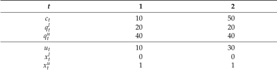
Example 1(Difference between the optimistic and the pessimistic variants). Suppose T=2, there is only one follower, the leaders’s average tariff is Q = 30, and the follower’s desired con- sumption is D^l = D^u = 1. Further data is depicted in Table 1. In the optimistic variant of the problem, the optimal tariff vector is q= (20, 40)for which the best response is x^o = (1, 0) giving an objective function value of 10. In contrast, in the pessimistic variant of the prob- lem, if u2−q2 ≥ u1−q1, the follower will load the second period with 1 unit of consumption, i.e., x^p= (0, 1), for which the leader’s objective function value is q2−50. Since20≤qt≤ 40 and q1+q2 ≤ 60, u1−q1 ≤ u2−q2for any feasible q. Thus the best option for the leader is q₂=40(with arbitrary q₁), and its objective function value is−10on x^p= (0, 1). Observe that with higher values of c2, the loss of the leader can increase arbitrarily.

Table 1.Data for Example1.

t 1 2

ct 10 50

q^l_t 20 20

q^u_t 40 40

ut 10 30

x^l_t 0 0

x^u_t 1 1

The next example shows that the pessimistic variant may not have an optimal solution, which justifies the supremum in (7).

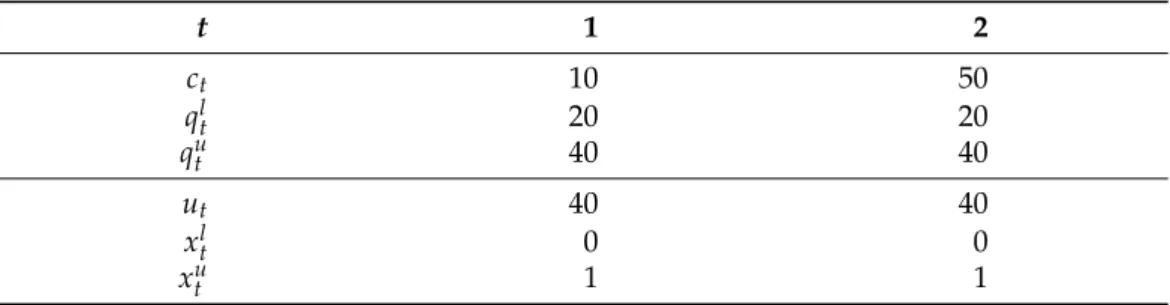
Example 2(No optimal solution for the pessimistic variant). Suppose T=2, there is only one follower, the leaders’s average tariff is Q=40, and D^l =D^u =1. Further data are depicted in Table2. The optimistic solution is q = (40, 40)and x^o = (1, 0), resulting in a profit of 30 for the leader. However, for q= (40, 40), the pessimistic answer would be x^p= (0, 1)for which the leader’s objective function value is−10. However, the leader can do much better by setting q= (40−e, 40). Then u−q= (e, 0); thus, the follower’s unique optimal solution is x^p= (1, 0) for which the leader’s objective function value is30−e. Clearly, the supremum of the leader’s objective function value is 30, but it cannot be attained by any feasible solution.

Table 2.Data for Example2.

t 1 2

ct 10 50

q^l_t 20 20

q^u_t 40 40

ut 40 40

x^l_t 0 0

x^u_t 1 1

4. Preliminaries

4.1. The Continuous Knapsack Problem

This section briefly overview the key properties of optimal solutions of the continuous knapsack problem as follows:

Maximize

∑

wtxt (8)

D^l ≤

∑

xt≤D^u

x^l_t≤xt≤x_t^u, t=1, . . . ,T, where 0≤x^l_t<x^u_t for allt. Note that thewtare not restricted in sign.

The continuous knapsack problem (8) admits a feasible solution if and only if∑t∈[T]x^l_t≤ D^u ≤ _∑t∈[T]x^u_t. When feasible, it always has a finite optimum, since all variables are bounded. Without loss of generality,D^l ≥_∑t∈[T]x^l_t.

Proposition 1. Suppose the continuous knapsack problem (8) admits a feasible solution. Then it has an optimal solution x^?of the following structure:

1. x^∗_t =x^l_tfor t∈L, x^∗_t =x^u_t for t∈U;

2. x^∗_p∈ {x^l_p,x^u_p,D^l_p−_∑t∈L∪Ux^∗_t,D^u_p−_∑t∈L∪Ux_t^∗}.

where L∪P∪U is a partitioning of[T]such that P={p}for some p∈[T], wt≥wpfor t∈U, and wt ≤ wpfor t ∈ L. Moreover, such a partitioning can be computed in O(TlogT)time by determining a permutationπsuch that w_π(t)≥w_π(t+1)for t=_{1, . . . ,}T−1.

4.2. General Properties of Optimal Solutions

Firstly, observe that without loss of generality, the lower bounds on the prices can be assumed to be 0.

Proposition 2. If q^l_t>0, then an equivalent problem can be derived by setting

• uit :=uit−q^l_tfor i=1, . . . ,m;

• ct:=ct−q^l_t;

• Q:=Q−q^l_t/T;

• q^u_t :=q^u_t −q^l_t;

• q^l_t:=0.

Proof. Let ˜qt = qt−q^l_t, while ˜qτ = qτ for τ ∈ [T]\ {t}. Substitutingqtwith ˜qt+q^l_t in (1)–(3) + (4)–(6) yields a formulation satisfying the properties of the statement.

From now on, the following assumption is made:

Assumption 1. q^l_t=0for all t∈[T], Q>0, and∑^Tt=1q^u_t ≥QT.

The minimum consumption of each followeriis at least∑t=1^T x^l_it, while the maximum consumption is at most∑^Tt=1x_it^u. Moreover, ifD_i^u = _∑^T_t=1x_it^l, then the followerihas a unique optimal solution, which is independent ofq. Hence, without loss of generality, the following assumption also holds:

Assumption 2. D^l_i ≥_∑^T_t=1x^l_it, and∑^Tt=1x^l_it <D_i^u≤_∑^T_t=1x^u_itfor each i.

Now, an easy observation can be made about the leader’s optimal price vector, which is valid in the optimistic and in the pessimistic variant of the bilevel tariff optimization problem.

Proposition 3. Let(q^?,x^?)be an optimal solution for (1)–(3) + (4)–(6) such that∑^Tt=1∑^mi=1x^?_it >

0. Then either q^?_t =q^u_t for some t∈[T], or∑^Tt=1q^?_t =QT.

Proof. Suppose q^? does not satisfy the conditions of the statement. Then for e > 0 sufficiently small, the price vector ˜q= (q^?₁+e, . . . ,q^?_T+e)is feasible, and induces the same partitioning of the time periods asq^?for each followeri; cf. Proposition1. Hence(q,˜ x^?) constitutes a feasible solution for (1)–(3) + (4)–(6), and

∑

(q˜t−ct)

∑

x_it^? =

∑

(q^?_t−ct)

∑

x^?_it+e

∑

∑

x_it^? >

∑

(q^?_t −ct)

∑

x^?_it,

where the last inequality follows from the assumption of the theorem. However, it follows that(x^?,q^?)is not an optimal solution, a contradiction.

5. Polynomially Solvable Special Cases with One Consumer Only

This section investigates the one-consumer special case (m = 1), and under some further restrictions, polynomial time algorithms are provided for solving the optimistic and pessimistic variants as well.

Throughout this section, it is assumed that the prices are unbounded; i.e.,q^u_t =∞for allt. In fact, by (2), it may equivalently be assumed thatq^u_t =QTfor allt. Further on, some assumptions on regularity are introduced in the next section.

Firstly, the optimistic variant is discussed in Section5.1, and the pessimistic one in Section5.2.

5.1. The Optimistic Variant

Let us assume thatD^l = D^u, and let Ddenote the common value. The case with D^l <D^uwill be discussed later.

Definition 1. A price vector q is feasible if it satisfies (2) and (3).

Definition 2. If D=D^l=D^u, then a time period t∈[T]is regular, if x^l_t< ^D

T <x^u_t.

Observation 1. If there is at least one regular time period, then D>_0.

Definition 3. From now on, an optimal solution (q^?,x^?) of (1)–(3) + (4)–(6) is called non- degenerate if q^?_t >0for all t∈[T].

In the following results, it is assumed thatx^?is an optimal solution of the contin- uous knapsack problem (8) for weightswt = ut−q^?_t, and it respects the conditions of Proposition1for some partitioningL∪P∪Uof[T], whereP={p}.

Lemma 1. Assume (1)–(3) + (4)–(6) admits a non-degenerate optimal solution(q^?,x^?), and sup- pose t∈L is a regular time period. Then

ut−q^?_t =up−q^?_p.

Proof. Let (_q^?_,x^?) be a non-degenerate optimal solution of (1)–(3) + (4)–(6) such that ut−q^?_t <up−q^?_p. Let

e=min{up−q^?_p−(ut−q^?_t),q^?_t}. Define a new price vector

˜

q=q^?₁+ ^e

T, ...,q^?_t −e+ ^e

T, ...,q^?_T+ ^e T

.

Then ˜qis a non-degenerate feasible solution of (1)–(3). Moreover,x^?is an optimal solution of the continuous knapsack problem (8) with weights ˜wt=ut−q˜t, as it satisfies the conditions of Proposition1 for the same partitioning L∪P∪U of [T]. However, the objective value (1) changes by

−e·x^l_t+ ^e TD.

Due to the regularity assumption

x_t^l< ^D T, the change in the objective value is positive:

−e·

x^l_t− ^D T

>0 which contradicts the optimality of(q^?,x^?).

Lemma 2. Assume (1)–(3) + (4)–(6) admits a non-degenerate optimal solution(q^?,x^?), and sup- pose t∈U is a regular time period. Then

ut−q^?_t =_up−q^?_p.

Proof. (sketch) Analogous to that of Lemma1. It is only mentioned that in this case

˜

q=q^?₁− ^e

T, ...,q^?_t +e− ^e

T, ...,q^?_T− ^e T

. The rest follows from the regularity assumption, i.e.,D/T<x_t^u.

Lemma 3. Suppose all time periods are regular, and (1)–(3) + (4)–(6) admits a non-degenerate optimal solution(q^?,x^?). Then

uτ−q^?_τ =

∑

t∈[T]

ut

T −Q, τ=1 . . . ,T.

Proof. Since ut−q^?_t = up−q^?_p for all t ∈ [T] by Lemmas 1 and2, it holds for any τ∈[T]that

T(u_τ−q^?_τ) =

∑

t∈[T]

ut−

∑

t∈[T]

q^?_t =

∑

t∈[T]

ut−Q·T,

where the second equation follows from Proposition3, since∑^Tt=1x^?_t =D>0, as each time period is regular.

Now, a necessary and sufficient condition is provided for the existence of a non- degenerate optimal solution. Letumin=min_t∈[T]ut.

Theorem 1. Assume that all time periods are regular. The bilevel tariff optimization problem (1)–(3) + (4)–(6) admits a non-degenerate optimal solution if and only if Q−(1/T)_∑t∈[T]ut+umin>0.

Proof. First suppose (1)–(3) + (4)–(6) admits a non-degenerate optimal solution(q^?,x^?). Then by Lemma3,q^?_t =ut−(1/T)_∑τ∈[T]u_τ+Q, and thusut−(1/T)_∑τ∈[T]u_τ+Q>0 for allt∈[T], and in particularu_min−(1/T)_∑τ∈[T]u_τ+Q>0.

In order the prove the converse direction, let us relax the bound constraints (3) for theqt

variables, i.e.,−∞<qt<∞. Note that this relaxation permits unbounded optimum value for the leader. However, as it is shown below, this is not the case. Fix some feasible price vectorq^?, and letx^?be the corresponding optimal solution of the follower respecting the partitioningL∪P∪Uof[T]given by Proposition1. If∑^Tt=1q^?_t <QT, then while increasing all coordinates ofq^?by the same value, the follower’s solutionx^?remains optimal, and the profit of the leader increases. Thus, without loss of generality,∑^Tt=1q^?_t = QT. Suppose P= {p}in the partitioning. Ifq^?fails to satisfyut−q^?_t =up−q^?_pfor somet∈ [T], then almost the same transformations can be applied as in Lemmas1and2to conclude that the leader’s objective function value can be improved:

• Ifut−q^?_t <up−q^?_p, thent∈L, andq^?_t is decreased bye−e/T, whileq^?_τis increased bye/Tfor allτ6=t, wheree=up−q^?_p−(ut−q^?_t).

• Ifut−q^?_t >up−q^?_p, thent∈U, andq^?_t is increased bye−e/T, whileq^?_τincreases by e/Tfor allτ6=t, wheree=ut−q^?_t −(up−q^?_p).

In either case, x^? remains optimal for the resulting price vector, and the leader’s objective function value strictly increases.

By repeating this transformation, a solution ˆqof the relaxed problem is derived such thatut−qˆt=up−qˆpfor allt∈[T], whilex^?remains optimal for ˆq. However, ˆqsatisfies

ˆ

qt =ut−(1/T)_∑τ∈[T]uτ+Qfor allt ∈ [T](see the proof of Lemma3). Consequently, ifu_min−(1/T)_∑τ∈[T]u_τ+Q > _{0, then}ut−(1/T)_∑τ∈[T]u_τ+Q > _{0 for all} t ∈ [T]_. Hence, ˆqis a non-degenerate feasible solution for the leader and (x^?, ˆq)has a strictly greater objective function value than(x^?,q^?). Since the above argument applies to any vector q^? with finite coordinates only, it can be deduced that umin−(1/T)_∑τ∈[T]u_τ+ Q > 0 implies that there exists a non-degenerate optimal solution of the bilevel tariff optimization problem.

Theorem 2. Suppose D^l = D^u, all time periods are regular, and (1)–(3) + (4)–(6) admits a non-degenerate optimal solution(q^?,x^?). Then

q^?_τ=u_τ− ¹

T

∑

t∈[T]

ut+Q, τ=1, . . . ,T.

Moreover, the optimal consumptions x^?can be obtained by solving the continuous knapsack problem:

Maximize

∑

(q^?_t −ct)xt

∑

xt=D

x^l_t≤xt≤x^u_t, t=1, . . . ,T.

Proof. The first part of the statement follows from Lemma3, and the second part from the optimality ofq^?.

Note that Theorem2yields an optimal solution for the optimistic variant of the bilevel tariff optimization problem. Then,x^?can be computed by using Proposition1.

Now, consider the more general case whenD^l <D^u. Definition 4. If D^l <D^u, then a time period t∈[T]is regular if

x^l_t< ^D

l

T and D^u T <x^u_t.

Theorem 3. Suppose D^l < D^u, all time periods are regular, and (1)–(3) + (4)–(6) admits a non-degenerate optimal solution(q^?,x^?). Then x^?satisfies

D^l ≤

∑

t∈[T]

x^?_t







=D^u if(1/T)_∑t∈[T]ut−Q>0,

≤D^u if(1/T)_∑t∈[T]ut−Q=0,

=D^l if(1/T)_∑t∈[T]ut−Q<0.

Proof. The first inequality follows from the feasibility of x^?. Defineq^?_t as in Theorem1.

Thenut−q^?_t = (1/T)_∑τ∈[T]u_τ−Qfor allt∈ [T]; i.e., the objective function coefficient of the follower is the same in all time periods. Hence, the follower’s optimal solution is chosen based on the leader’s objective function∑t∈[T](q^?_t −ct)xt. That is, the follower solves (8) with

Clearly, if(1/T)_∑τ∈[T]uτ−Q < 0, then in any optimal solution of the follower, the periods are loaded to the least possible extent untilD^lis reached, since all objective function coefficients (of the follower) are negative. Therefore, since the follower chooses an optimal solution which maximizes the leader’s objective function value, the follower solves (8) with cost vectorwt:=q^?_t −ctfort∈[T], whileD^u is replaced withD^l. Analogously, if(1/T)_∑τ∈[T]u_τ−Q>0, then in any optimal solution of the follower, the periods are loaded to the maximal possible amount untilD^uis reached. Therefore, the follower solves (8) with cost vectorwt:=q^?_t−ctfort∈[T], whileD^lis replaced withD^u.

Finally, if (1/T)_∑τ∈[T]u_τ−Q = 0, then the follower chooses its optimal solu- tion solely by considering the objective function of the leader—namely, it solves the fractional knapsack problem (8) with weightswt := q^?_t −ct. The result follows from Proposition1.

5.2. The Pessimistic Variant

Under the conditions of Theorem2, the optimum value of the pessimistic variant (where (1) is replaced with (7)) can be approximated by a slight perturbation of the optimal price vector for the optimistic variant.

Definition 5. Let q be any feasible price vector, andπ a permutation of (1, . . . ,T)such that q_π(t)−c_π(t) ≥ q_π(t+1)−c_π(t+1)for t = 1, . . . ,T−1. For any δ > 0, the price vector q^δ defined by

q^δ_π(t)= ^QT

T(Q−δ(T−1)_/2)(q_π(t)−(T−t)δ), t=1, . . . ,T, is called theδ-perturbation ofq.

Theorem 4. Suppose that all time periods are regular, and (1)–(3) + (4)–(6) admits a non- degenerate optimal solution(q^?,x^?)such that∑^T_t=1x^?_t >0. Then for anye>0, there existsδ>0 such that for the price vector(q^?)^δobtained by theδ-perturbation of q^?, the follower has a unique optimum x^δand∑^Tt=1((q^?)^δ_t−ct)x^δ_t ≥_∑^T_t=1(q^?_t −ct)x^?_t −e.

Proof. By assumption, the conditions of Proposition3are satisfied, so∑^Tt=1q^?_t = Q·T.

Then, it holds that

∑

(q^?)^δ_t = ^QT

T(Q−δ(T−1)/2)(QT−

T−1

∑

k=0

kδ) =QT.

For a sufficiently smallδ,(q^?)^δ ≥0, sinceq^?_t >0 for alltby assumption. Moreover, all the valuesut−(q^?)^δ_tare different, andut−(q^?)^δ_t >u_k−(q^?)^δ_kif and only ifq^?_t −ct>

q^?_k−ck. It follows that for the price vector(_q^?)^δ, the follower will prefer the time periods with higherq^?_t−ctvalues. On the one hand,x^?is an optimal solution of the follower for the price vector(q^?)^δ. On the other hand, since(q^?)^δ_t ≥q^?_t −(T−1)δ, the decrease of the objective function value of the leader is at most

(T−1)δ

∑

x^?_t = (T−1)δD.

Therefore, forδ=_e/((T−1)D), the leader’s objective function value decreases by at moste, as claimed.

If the conditions of Theorem4are not satisfied, then the more general Theorem5can be applied to obtain a suboptimal solution of the pessimistic variant of the bilevel tariff optimization problem; see Section6.2.

6. The General Case with Multiple Consumers 6.1. Solution of the General Optimistic Variant

This section presents an equivalent single-level MILP formulation for the optimistic variant of the bilevel tariff optimization problem, for arbitrary number of followers. No restrictions are imposed on the problem data, except Assumptions1and2.

The MILP is derived from a reformulation of the followers’ problems using the familiar complementary slackness conditions of linear programming at the expense of using new binary indicator variables. Moreover, the quadratic term∑^Tt=1∑^mi=1qtx_it that appears in both the leader’s and the followers’ objective functions is substituted with an equivalent linear expression from the equivalence of the followers’ primal and dual objective functions.

Let us start by formalizing the dual of the linear program (4)–(6) of followeri∈ {1, . . . ,m} using dual variablesα⁺_i andα_i⁻for the lower and upper bounds on∑^Tt=1x_itin constraint (5), respectively, andβ⁺_it andβ⁻_it for the lower and upper bounds onx_itin constraint (6):

MinimizeD^u_iα⁺_i −D^l_iα⁻_i +

∑

(x^u_itβ⁺_it −x^l_itβ⁻_it) (9)

subject to

α⁺_i −α⁻_i +β⁺_it −β⁻_it =u_it−qt, t∈[T] α⁻_i ,α⁺_l ,β⁻_it,β⁺_it ≥0 t∈[T]

Now, strong duality of linear programs (LP) is exploited—that is, the optimum ob- jective function values of the primal and the corresponding dual LP are equal, provided a finite optimum exists for either of them. Since the primal LP of each follower always admits a finite optimum, the following holds:

∑

(uit−qt)xit =D^u_iα⁺_i −D_i^lα⁻_i +

∑

(x^u_itβ⁺_it −x^l_itβ⁻_it)

Hence,

∑

qtxit =

∑

uitxit−D_i^uα⁺_i +_D^l_iα⁻_i −

∑

(_xit^uβ⁺_it −x^l_itβ⁻_it)

Consequently, the optimistic variant of the bilevel tariff optimization problem can be equiva- lently described by the following mathematical problem with complementarity constraints:

Maximize

∑

∑

(uitxit−x^u_itβ⁺_it +x^l_itβ⁻_it −ctxit) −

∑

(D_i^uα⁺_i −D^l_iα⁻_i ) (10) subject to

∑

qt≤T·Q,

q^l_t≤qt≤q^u_t, t∈[T] 0≤α⁺_i ⊥D^u_i −

∑

xit≥0, i∈[m]

0≤α⁻_i ⊥

∑

x_it−D^l_i ≥0, i∈[m]

0≤β⁺_it ⊥x^u_it−xit ≥0, i∈[m], t∈[T] 0≤β⁻_it ⊥x_it−x^l_it ≥0, i∈[m], t∈[T] α_i⁺−α⁻_i +β⁺_it −β⁻_it =u_it−qt, i∈[m], t∈[T]

where 0≤ L⊥R≥ 0 denotes thatL ≥0,R ≥0, and eitherL=0, orR =0. The latter complementarity constraint can be described by two linear constraints using an extra binary variable and some big Mconstant, which is a standard rewriting technique. One issue with this transformation is the choice of the bigMconstant. In the above mathematical program, theD_i^u,∑^Tt=1x^u_it−D_i^l,x^u_it, andx^u_it−x^l_itwill do for the correspondingRexpressions.

However, in theLexpressions, the maximum values of theα⁺_i ,α⁻_i ,β⁺_it, andβ⁻_it variables have to bound in the optimal solutions. Since the primal program (4)–(6) always has a finite optimum for each followeri, the dual LP (9) always admits a basic optimum solution. It is not hard to see that the values ofα⁺_i andβ⁺_it are bounded by maxtu_it, provided this quantity is non-negative; otherwise, they are 0. Forα⁻_i andβ⁻_it, the upper bound is maxt(q^u_t −u_it), provided this quantity is positive, and otherwise 0.

6.2. Solution of the General Pessimistic Variant

In the pessimistic variant of the bilevel tariff optimization problem, the followers are adversarial toward the leader. Suppose the tariff vectorqis fixed by the leader. By Proposition1, each followeriloads the periods in non-increasinguit−qtorder. In case of ties, the period with smallerqt−ctvalue must be loaded first. Hence, followeriloads the time periods in the order given by the permutationπ_i of {1, . . . ,T}satisfying the following conditions:

• Eitheru_iπi(t)−q_πi(t)>u_iπi(t+1)−q_πi(t+1), or

• u_iπi(t)−q_πi(t) = u_iπi(t+1)−q_πi(t+1), and q_πi(t)−c_πi(t) ≤ q_πi(t+1)−c_πi(t+1) for t=1, . . . ,T−1.

The next goal is to characterize the optimal solution of the followers. First suppose that D^l_i =D^u_i:

Proposition 4. For a fixed price vector q, let permutationπ_i be defined as above. If D^l_i = D_i^u, then the optimal solution of follower i has the following structure: There exists an index k such

that x_iπi(t)=x^u_iπ

i(t)for t∈[1,k], x_iπi(k+1)=D_i^l−_∑^k_t=1x^u_iπ

i(t)−_∑t=k+2^T x^l_iπ

i(t), and x_iπi(t)= x^l_iπ

i(t)for t∈[k+_2,T].

Proof. By definition,u_iπi(t)−q_πi(t) ≥ u_iπi(t+1)−q_πi(t+1)fort < T. Hence, the follower maximizes its profit by saturating thex_itin the order given byπ_i, which at the same time minimizes the objective function of the leader for the fixed price vectorq.

Now, consider the case whenD^l_i <D^u_i. Let the vectors

x¯_i ∈R^{Tand ¯x}i ∈R^{Tbe the} optimal solutions of followeriwhen the total consumption must be equal toD^l_i or D_i^u, respectively.

Proposition 5. For a fixed price vector q, let permutationπ_i be defined as above. If D^l_i < D_i^u, then the optimal solution of follower i has the following structure: there exists an index k such that x_iπi(t)=x¯_iπi(t)for t∈[1,k], and x_iπi(t)=

x¯_iπi(t)for t∈[k+1,T]. Moreover, k=T unless there exists an index t such that either u_iπi(t)−q_πi(t)=0and q_πi(t)−c_πi(t)>0, or u_iπi(t)−q_πi(t)<0, in which case(k+₁)is the smallest index with this property.

Proof. First, suppose thatk=T. Then followeriwill certainly assign the largest possible consumption tox_iπi(t)ifu_iπi(t)−q_πi(t)>0. Moreover, in all the positionstwithu_iπi(t)− q_πi(t)=0, if any, it holds thatq_πi(t)−c_πi(t)≤0, sincek=T, and then again, followeriwill maximize thex_iπi(t). In both cases, the maximum consumption is reached by settingx_iπi(t) to ¯x_iπi(t). Finally, sincek=T, there can be notsuch thatu_iπi(t)−q_πi(t)<0.

Now supposek < T. Then, in positionk+1, eitheru_iπi(k+1)−q_πi(k+1) = 0 and q_πi(k+1)−c_πi(k+1) > 0, or u_iπi(k+1)−q_πi(k+1) < 0 holds. The best option for follower iis to maximize the consumption x_iπi(t)for t ∈ [1,k], i.e.,x_iπi(t) = x¯_iπi(t)for t ∈ [1,k]. However, to maximize its utility, and minimize the leader’s profit, from positionk+1 on, it has to assign the least possible amount to get a feasible solution, and accordingly, fort=_k+_{1, . . . ,T,xiπ}

i(t)=

x¯_iπi(t).

The above propositions can easily be turned into algorithms; the details are omitted.

Definition 6. It is said that(q^?,x^?)satisfies the optimality conditions if x^?_i fulfills the conditions of Proposition4if D^l_i =D_i^u, or Proposition5if D^l_i <D^u_i, for i∈[1,m]; q^?satisfies the optimality conditions of Proposition3.

Lemma 4. Fix someε>0. If an optimal solution(x^?,q^?)of the optimistic variant of the bilevel tariff optimization problem is such that either q^?_t <q^u_t for all t, or q^?_t >0for all t, then the price vector q^?can be slightly perturbed such that x^?becomes the unique optimal solution of the followers for the modified price vector, and the objective function value of the leader decreases by less thanε.

Proof. First supposeq^?_t <q^u_t for allt. Letσbe a permutation of[T]such thatq^?_σ(t)−c_σ(t)≥ q^?_σ(t+1)−c_σ(t+1)fort=1, . . . ,T−1. Define ˜q_σ(t):=s·(q^?_σ(t)+δ^(T−t+1))fort∈[T], where δ>0 is a parameter, andsis a scaling factor such that∑^Tt=1q˜t=QT. Forδsufficiently small,

˜

qis feasible for the leader, and ifuit−q^?_t > u_ik−q^?_k, thenuit−q˜t > u_ik−q˜_k. Moreover, ifuit−q^?_t = u_it⁰−q^?_t0, andq^?_t −ct > q^?_t0−c_t⁰ for somet 6= t⁰, then ut−q˜t > u_t⁰−q˜_t⁰. Hence, for ˜q, both the optimistic and the pessimistic answers of the followers are equal to x^?. Finally,

∑

∑

(q˜t−ct)x_it^? ≥

∑

∑

(q^?_t−ct)x^?_it−e for a sufficiently smallδ.

Now supposeq^?_t > 0 for allt. Then a very similar transformation can be applied, but this time the prices are decreased by some power ofδ>0 sufficiently small; the details are omitted.