1.Introduction CHALLENGESOFLOCALIZATIONALGORITHMSFORAUTONOMOUSDRIVING

(1)

hjic.mk.uni-pannon.hu DOI: 10.33927/hjic-2020-07

CHALLENGES OF LOCALIZATION ALGORITHMS FOR AUTONOMOUS DRIVING

HUNORMEDVE^*1ANDDÉNESFODOR¹

1Research Institute of Automotive Mechatronics and Automation, University of Pannonia, Egyetem u. 10, Veszprém, 8200, HUNGARY

One could easily believe that the technology surrounding us is already easily capable of determining the current location of a vehicle. Whilst many devices, technologies, mathematical models and methods are available in the automotive world, the complexity of the localization problem still cannot be underestimated. The expectation is to determine in real time with a high degree of accuracy the location of a vehicle in order to make correct autonomous decisions and avoid dangerous and potentially damaging situations. Various research directions have been undertaken since the birth of autonomous driving from the well-known satellite navigation-based systems that rely on offline maps to the more sophisticated approaches that use odometry and existing sensor data using sensor fusion. The aim of the current work is to review what has been achieved so far in this field and the challenges ahead, e.g. the need for a change in paradigm as today’s global positioning systems are not intended for machines but humans and are based on the abstraction of human thinking and human decision-making processes.

Keywords: autonomous driving, localization, information fusion, filtering

1. Introduction

Vehicle localization is one of the four functions of autonomous vehicle navigation, namely mapping, localization, motion and interaction, which are the answers to the four basic questions concerning navigation: Where am I?

Where can I move to? How can I do it? How do I inter- act? If a vehicle is to navigate as expected, these functions need to operate correctly [1]. Historically, the purpose of in-car localization was driver assistance in the form of helping the driver to navigate. Such systems that are currently in use provide information, with some degree of accuracy, to the driver and then the driver makes decisions based on the information, which can either be accepted and acted upon or rejected in the form of proceeding in another direction. In the case of autonomous driving, it is quite clear that simply rejecting position information since the main control algorithm is not an option as this is the only item of data to be used, therefore, it must be used and a decision made based on it. This raises the question of certainty.

The requirement to operate safely anywhere and at anytime makes the performance measures far stricter than ever before. The performance measures are [2]:

Accuracy the degree of conformity of position information provided by the localization system relative to actual values.

*Correspondence:medve.hunor@mk.uni-pannon.hu

Integrity a measure of trust that can be implemented in the information from the localization, which is the likelihood of undetected failures given the specified accuracy of the system.

Continuity of service the probability of the system con- tinuously providing information without nonsched- uled interruptions during the intended working pe- riod.

Availability the percentage of time during which the service is available for use taking into account all the outages irrespective of their origins. The service is available if the requirements concerning accuracy, integrity and continuity are satisfied.

Over the last 10-15 years, the number of sensors and related advanced driver-assistance systems in passenger vehicles has increased. The primary task of each of these sensors and services is to observe a segment of the surroundings and its status, then assist the driver in that regard. Since the data from a single sensor does not contain all the information about the vehicle’s surroundings, fur- ther information concerning its absolute location cannot be extracted based on a single sensor. In fact, the sensors provide complementary information and through information fusion the vehicle’s absolute location and status can be obtained. This is shown inFig. 1.

The main groups of information sources are the following:

(2)

Figure 1:The concept of information fusion

• Global Navigation Satellite Systems (GNSS)

• Traditional vehicle sensors:

– Odometer

– Wheel speed sensor – Steering angle sensor

• Inertial Measurement Unit (IMU):

– Accelerometer – Gyroscope

• Optical, sound- and radio-based sensors:

– Radar

– Ultrasonic sensors – Vision sensors

– LiDAR (Light Detection and Ranging)

• Vehicle models with various levels of complexity

• Databases; offline or cloud-based:

– Maps

– Traffic situation

• Dedicated short-range communication:

– Vehicle-to-vehicle (V2V) – Vehicle-to-infrastructure (V2I).

It is important to note that none of these information sources are ideal and error-free. The errors will propagate through the sensor fusion algorithm, moreover, affect the end result and the previously described figures of merit.

The following sections address each device family then the fusion methods are analysed.

2. Information Sources

2.1 Global Navigation Satellite Systems

The global navigation satellite system (GNSS) is a radio positioning-based technology using satellite infrastructure that aims to achieve global coverage. Historically, satellite-based sytems have been considered as the core element of localization. Currently, a number of systems are in operation, the major ones are GPS (USA), BeiDou (China), GLONASS (Russia) and Galileo (EU).

Every satellite broadcasts a specific signal and its position. The spectral range of the signals is1.2−1.6GHz, utilising frequency bands of between2and40MHz. Any user equipped with a GNSS receiver receives the signal and measures the signal propagation delay, then estimates

the range of distance from it. By using signals from at least four satellites, the receivers can reduce the estimate to intercept the ranges from each satellite, which basi- cally provides a potential location within the range in terms of geospatial coordinates. It is important to note that the position information is useful only if used together with maps which put the information in context.

Even though the accuracy of receivers is increased by various augmentation systems, issues resulting from poor satellite constellations, signal blockage and multi- path propagation in urban environments cannot be ex- cluded. For this reason, safety-critical applications cannot solely rely on GNSS technology.

Although satellite-based systems are far from perfect, they are and will continue to be the single most important information source of any localization algorithm.

2.2 Vehicle Model

Models representing the dynamic model of a vehicle’s range from the simple spring-mass model to a complex multibody multi-level model. A well-known and used model is the single track model [3] with a number simpli- fications, however, it provides a reasonable solution for modeling lateral dynamics, therefore, it forms the core of the electronic stability program (ESP) of many vehicle manufacturers. The inputs of the single track model are lateral acceleration, longitudinal speed and yaw rate, which are provided by the relevant sensors as discussed inSection 2.3.

Another element in a complex model is the tire model which is assumed to be the only part in contact with the road. These models, e.g. Pacejka’s Magic Formula [4], are often semi-empirical.

It is important to note that a more detailed model requires more parameters which, in the case of inaccu- rate identification, may impact the overall accuracy of the model’s output.

2.3 Traditional Vehicle Sensors and Inertial Measurement Unit (IMU)

A wide range of traditional vehicle sensors have already been installed in most vehicles, moreover, analogue measurements are already being processed digitally. Most of them provide basic information to human drivers directly, e.g. the odometer, whilst others are parts of safety fea- tures. For autonomous driving, exactly the same information is also required.

Wheel speed sensors mounted in the wheel drum provide vital inputs to the anti-lock braking system by sens- ing the movement of the circumference of each tire in a passive or active setting.

Steering angle sensors are mounted on the steering shaft and measure the steering wheel angle, their outputs are interpreted as the intended direction of the vehicle, which is a key input to the electronic stability program (ESP).

(3)

Accelerometers measure the acceleration of the vehicle on the specified axis, multi-axis accelerometers are also in use. They are primarily used for inertial navigation in combination with yaw-rate sensors.

Yaw-rate sensors, often referred to as gyroscopes, measure the rotation of the vehicle along the vertical axis.

Such a sensor provides an input to the single track vehicle model in conjunction with the ESP.

Accelerometers and yaw-rate sensors integrated in one cluster comprise the inertial measurement unit (IMU).

2.4 Optical as well as Sound- and Radio- Based Sensors

In automotive radar systems, a distinction is made between short range radar (SRR) and long range radar (LRR). The detection range of short range radar is from 0.2to50meters with a detection angle of±35^◦, whilst that of the long range radar is from2to150meters with a detection angle of±6^◦. SRR is predominantly used in anti-collision and parking aid systems.

Radars are able to detect multiple objects as well as measure distance, relative speed and the angle to an object simultaneously. LRR is typically applied in adaptive cruise control and collision avoidance. Radar technology is affected by the weather and functionality cannot be guaranteed in extreme conditions. Overall information from radars can complement other location-related information sources.

Vision sensors are primarily used in vehicles to detect and possibly recognise its surroundings, e.g. other vehicles, obstacles, pedestrians and landmarks, which are potentially useful pieces of information for a localization algorithm.

Charge-coupled (CCD) and complementary metal ox- ide semiconductor (CMOS) devices are the main sensor technologies applied in digital cameras to generate an image of the surroundings, in fact both are semiconductor devices.

In CMOS devices, every pixel has its own charge-to- voltage conversion and digitalization, so their outputs are digital signals. Pixels that perform their own charge-to- voltage conversion decrease their uniformity and image quality as well as remove a useful area from light capture.

In CCD sensors, a pixel’s charge signal is sent through a limited number of outputs to be converted into voltage and then transmitted out of the chip as an analogue signal to be processed and digitalized. This requires more time and energy when compared to CMOS sensors, however, results in a higher quality but less noisy image. As the CMOS manufacturing process is cheaper, recent devel- opments have focused on overcoming the drawbacks of CMOS sensors.

Ultrasonic sensors transmit higher frequency sound waves and evaluate the echo received by the sensors. The sensors also measure the elapsed time between sending and receiving back the signal, then calculate the distance

from the object. The types currently used in the automotive industry are able to measure within the range of 0.2 to 1.5 meters, with a horizontal angle of±60^◦and a vertical angle of ±30^◦, and are primarily used in parking aids. Nevertheless, the use of such sensors might provide useful inputs for a localization algorithm under given cir- cumstances.

LiDAR (Light Detection and Ranging) measures the distance of an object by emitting laser light and detecting the returning light. The differences in return times and wavelengths then provide the basis for a 3D representa- tion of the surroundings.

2.5 Databases and Maps

Maps stored in digital format differ from the classical map representations intended to be read by humans. Dig- ital road maps are comprised of nodes and arcs connect- ing the nodes. Arcs are represented in a discrete form and every node and shape point on the arc has geospatial coordinates linked to them. They are often represented as planar models in applications currently on the market.

2.6 Dedicated short-range communications

For any vehicle to communicate with either the infrastructure (vehicle-to-infrastructure: V2I) or with another vehicle (vehicle-to-vehicle: V2V), it is assumed that a suitable wireless protocol is in place, which allows bidi- rectional information flow in real time when a vehicle is travelling at high speed and is able to simultaneously han- dle multiple vehicles. Based on these assumptions, only applications related to localization are considered here.

The main purpose of V2I communication is to sup- port applications that target safety and mobility. Safety applications mainly consist of alerts and warnings, while mobility applications collect data from vehicles in order to capture the actual state of the traffic and provide such information to vehicles.

V2V applications determine the state of other nearby vehicles through the transmission of one or several mes- sages. Overall, the location-related content of these mes- sages alone might be insufficient for a vehicle to determine its own location, but can still provide useful complementary information to fusion algorithms.

3. Fusion Algorithms

The purpose of information fusion is to obtain more information from the sources than what is accessible from each individual source. This is achieved by combining sources which are complementary, moreover, the use of partially redundant sources reduces the ambiguity of the measured data which, overall, improves the performance of the system.

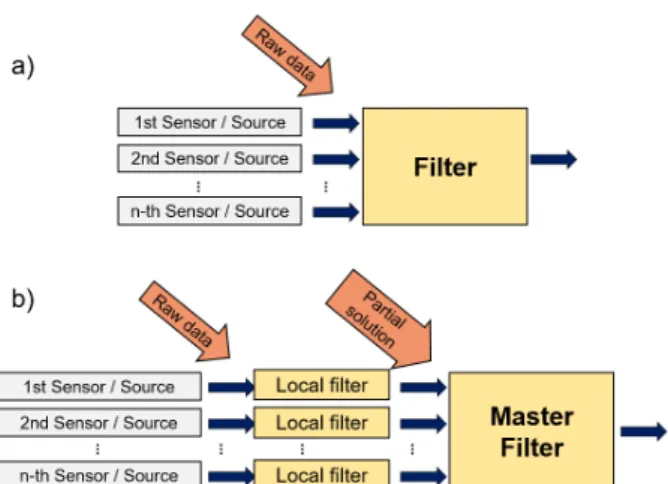
Fusion algorithms can be realized in either centralized or decentralized structures, as is shown in Fig. 2.

(4)

Figure 2:Filtering structures: a) centralized, b) decentralized

As the name suggests, in centralized structures, one filter performs the filtering of all signals which yields the benefit of minimal information loss as everything is directly available to the filter, while the amount of data to be processed in real time might imply an impractical degree of computational complexity. This is addressed by decentralized filters as every signal is filtered separately before being processed by a master filter. The computational load in general would be significantly less for one filtering unit, however, at the expense of partial information loss and reduced estimation accuracy.

In this chapter, selected filtering methods are presented: a conventional and widely used localization method, as well as a linear and a non-linear filtering method. Advanced filtering methods require prior knowledge of the system model and dynamics, the type of noise and their probability density functions as these are core elements to design a high-performance filter. The filtering algorithms presented in the following sections are used by the scientific community in various forms but often altered when compared to their originally published format (Kalman filter in [5], particle filter in [6]), in order to better suit the actual problem. In this paper, the thought process of [7] is followed.

3.1 Simple Algorithms: Dead Reckoning, In- ertial Navigation and Map Matching

The conventional localization algorithm consists of two steps; the first is the GNSS which defines the coordinates, the second is to match the given coordinates to a map.

This is shown inFig. 3.

The process of calculating the position based on its previously known position, elapsed time and speed is referred to as dead reckoning [8]. Inertial navigation is a very similar concept where the position is calculated based on data from accelerometers and gyroscopes, also referred to as dead reckoning based on inertial sensors.

In the following sections, no specific distinction is made between dead reckoning and inertial navigation.

Figure 3:Conventional localization algorithm

Traditional vehicle sensors and the inertial measurement unit (IMU) provide information about either the first or second order derivatives of the position of the vehicle together with the odometer which measures the distance travelled. All the data provided is relative to the starting position, therefore, none of the sensors provide information about its absolute position. In addition, all data will be incorporated into the coordinate system of the vehicle since all the sensors are mounted on the vehicle, therefore, coordinate transformations to the main coordinate system, which are used for the localization, are required.

The measured values are integrated by taking into consid- eration an initial position and, over time, the errors will be accumulated as part of the integration. It is important to note that the extent to which the error can increase is infinite. Despite such a disadvantage, the popularity of the method lies in the fact that it does not rely on external sources of information and the update rate is determined by the system itself, which overall defines the complementary nature of inertial navigation to GNSS.

Map matching is the process of identifying on the map the coordinates given by the GNSS on the map. On digital road maps, the road network is represented in a discrete form as nodes and arcs which connect nodes, each of which has geospatial coordinate information linked to it. The purpose of the map matching algorithm is to match the GNSS coordinates to the road map. It is highly likely that the map will not contain the exact coordinates defined by the GNSS and inertial navigation, therefore, it has to be matched to one of the few possible ones. Map matching algorithms assign probabilities to each possible location based on a set of information including previous locations, speed and heading of the vehicle, subsequently the evaluation is concluded based on these probabilities. Such algorithms can provide useful inputs to assist a human driver, however, it is easy to realize that rarely rarely can they provide sufficiently reliable inputs for autonomous driving. This creates the need for more reliable algorithms, which are normally more complex and require more computational power.

3.2 Linear Filtering: The Kalman Filter

The Kalman filter is a useful engineering tool in many in- dustries and control applications ranging from robotics, automotive, plant control, aircraft tracking and navigation. In general, they are relatively easy to design and code with an optimal degree of estimation accuracy for linear systems with Gaussian noise.

Let us describe a linear system with the following dis-

(5)

crete state-space model equations:

x_k =A_k−1x_k−1+B_k−1u_k−1+w_k−1

yk=Ckxk+vk (1) wherekin subscript refers to states and measurements at each discrete time instant andk−1in subscript to those at the previous time instant,xkdenotes the vector of the state variable,uk stands for the input or control vector, yk represents the output vector,Ak refers to the system matrix,BkandCk denote the input and output matrices, wk andvkstand for the process and measurement noise, respectively, which are white with Gaussian distribution and zero mean, andRk andQk are known covariance matrices.

wk ∼(0, Rk) vk∼(0, Qk) E

wkw_j^T

=Qkδk−j

E vkv^T_j

=Rkδk−j

E wv^T_j

= 0 (2)

whereδ_k−j is the Kronecker delta function (δ_k−j = 1, if k=jandδ_k−j= 0, ifk6=j). The aim is to estimate the system statexkby knowing the system dynamics and the noisy measurementsyk. The available information for the state estimation always depends on the actual problem at hand. If all measurements are up to date and accessible, includingkth, then a posteriori estimation can be computed, which is denoted byxˆ⁺_k. The meaning of the “+”

sign in superscript means the estimation is an a posteriori estimation.

The best way to estimate the a posteriori estimation is by computing the expected value ofxkconditioned to all measurements up to now, includingkas well.

ˆ

x⁺_k =E[xk|y1, y2, . . . , yk] (3) If all measurements, apart from k, are accessible, then the a priori estimate can be computed, denoted byxˆ⁻_k, where the “−” sign in superscript denotes the a priori estimate.

The best way to estimate the a priori state estimate is if the expected value ofxkconditioned to all measurements up to now, excludingk, is computed:

ˆ

x⁻_k =E[x_k|y₁, y₂, . . . , y_k−1] (4) It is important to note thatˆx⁻_k andxˆ⁺_k are estimates of the same quantity, before and after the actual measurement is obtained, respectively. Naturally, it is expected thatxˆ⁺_k is a more accurate estimate as more information is available.

At the beginning of the estimation process, the first measurement is obtained atk= 1, therefore, the estimate ofxˆ⁺₀ (k= 0) is given by computing the expected value ofx0:

ˆ

x⁺₀ =E[x0] (5)

Estimation of the error covariance is denoted by Pk, therefore,P_k⁻ represents the estimation of the error covariance of the a priori estimatexˆ⁻_k andP_k⁺ stands for the estimation of the error covariance of the a posteriori estimationxˆ⁺_k:

P_k⁻ = Eh

xk−xˆ⁻_k

xk−xˆ⁻_kTi P_k⁺ = Eh

xk−xˆ⁺_k

xk−xˆ⁺_kTi

(6) The estimation process starts by computing xˆ⁺₀, which is the best available estimate at this time instant for the value ofxˆ⁺₀. Ifxˆ⁺₀ is known,xˆ⁻₁ can be computed as follows:

ˆ

x⁻₁ =A0xˆ⁺₀ +B0u0 (7) then the general form to computeˆx⁻_kcan be established:

ˆ

x⁻_k =A_k−1xˆ⁺_k−1+B_k−1u_k−1 (8) This is referred to as time update from time instants (k−1)⁺ to k⁻. No new measurement information is available between the two, therefore, the state estimation propagates from one time instant to the other, and all state estimations are based on knowledge of the system dynamics. The time update is often referred to as the prediction step.

The next stage is to computeP, the estimation of the error covariance. The process starts by computing P₀⁺ which is the error covariance ofxˆ⁺₀. If the initial state is perfectly known, thenP₀⁺= 0; if no information is available, thenP₀⁺ =∞I. In general, the meaning ofP₀⁺is the uncertainty regarding the initial estimation ofx₀:

P₀⁺=Eh

x0−xˆ⁺₀

x0−xˆ⁺₀^Ti

(9) IfP₀⁺is known, thenP₁⁻can be computed as follows:

P₁⁻ =A₀P₀⁺A^T₀ +Q₀ (10) Based on the above, the generic form of the time update ofP_k⁻can be stated:

P_k⁻=A_k−1P_k−1⁺ A^T_k−1+Q_k−1 (11) So far, thetime update step has been presented, which is based on the system dynamics. The next step is the measurement update, where new information is obtained from the measurements. Using the logic from the method of recursive least squares, the availability of the measurementyk changes the value of the constantxin the following way:

K_k = P_k−1C_k^T C_kP_k−1C_k^T+R_k⁻¹

=P_kC_k^TR⁻¹_k−1 ˆ

xk = ˆx_k−1+Kk(yk−Ckxˆ_k−1)

P_k = (I−K_kC_k)P_k−1(I−K_kC_k)^T +K_kR_kK_k^T =

= P_k−1⁻¹ +C_k^TR⁻¹_k C_k⁻¹

=

= (I−KkCk)Pk−1 (12)

(6)

wherexˆ_k−1 denotes the estimation andP_k−1stands for the the estimation of the error covariance before processing measurementyk, therefore, xˆk andPk refer to the same informaton but afterykhas been processed.

If the logic ofxˆ_k−1→xˆ⁻_k andxˆ_k→xˆ⁺_k (a priori and a posteriori, respectively) is applied and the aforementioned equation reformulated, the a posteriori estimation is produced:

K_k = P_k⁻C_k^T C_kP_k⁻C_k^T+R_k⁻¹

=P_k⁺C_k^TR_k⁻¹ ˆ

x⁺_k = xˆ⁻_k +K_k(y_k−C_kˆx⁻_k)

P_k⁺ = (I−KkC_k)P_k⁻(I−KkC_k)^T +K_kR_kK_k^T =

= h

P_k⁻−1

+C_k^TR⁻¹_k C_ki−1

=

= (I−KkCk)P_k⁻ (13) These are the equations for the Kalman filtermeasure- ment updateora posterioriestimation. The matrixKkis often referred to as the Kalman gain.

By summarising the Kalman filtering algorithm, after initiation, the a priori estimate for every time instant k is given by:

ˆ

x⁻_k = A_k−1xˆ⁺_k−1+B_k−1u_k−1

P_k⁻ = A_k−1P_k−1⁺ A^T_k−1+Q_k−1 (14) and the a posteriori estimation is given by:

Kk = PkC_k^TR⁻¹_k−1 ˆ

x⁺_k = xˆ⁻_k +K_k(y_k−C_kxˆ⁻_k)

P_k⁺ = (I−KkCk)P_k⁻ (15) The aforementioned Kalman filtering algorithm is the optimal state estimator for linear systems with Gaussian unimodal noise processes, however, most real-world systems are nonlinear and, in many cases, with multimodal non-Gaussian noise, include a probability density function. A number of variations of Kalman filters devel- oped by the scientific community are trying to address the problem of nonlinearity. Most of them rely on the basic concept of Kalman filters using nonlinear adaptations, e.g. the extended Kalman filter which, at its core, is still a linear filter.

In general, versions of the nonlinear Kalman filter are considered to estimate accuracy well but are often poor compared with the theoretically optimal accuracy, with a real-time computational complexity in the order ofd³ whereddenotes a dimension of the state vector [9].

3.3 Nonlinear Filtering: The Particle Filter

Given the concerns about the estimation accuracy of versions of Kalman filters, true nonlinear filters or estimators are needed. The particle filter is a statistics-based estimator where at every discrete time instant, a number of state vectors, referred to as particles, are assessed with

regard to how likely they are to be the closest to the actual state. The mathematical formulation of the aforementioned idea is summarized in this section.

Let us describe a nonlinear system using the following equations:

xk+1 = fk(xk, wk)

y_k = h_k(x_k, v_k) (16) wherek denotes discrete time instants, x_k andy_k rep- resent the state and measurement, respectively, and w_k andvk stand for the noises of the system and measurement, respectively. The functionsfk(·)andhk(·)are a time variant nonlinear system and a measurement function, respectively. The noises of the system and measurement are assumed to be white and independent from each other with known probability density functions.

The aim of the generic Bayes estimator is to ap- proximate the conditional probability density functionxk

based on measurementsy1, y2, . . . , yk. This conditional probability density function is denoted as follows:

p(xk|Yk) =xk (17) conditioned on measurementsy₁, y₂, . . . , y_k. The particle filter is the numeric implementation of the Bayes estimator, in the following section this will be described.

At the beginning of the estimation, it is assumed that the probability density function ofp(x₀)is known, then N number of state vectors based on the probability density function of p(x0) are randomly generated.

These state vectors are the particles and are denoted by x⁺_0,i(i= 1, . . . , N). The value of N can be chosen arbitrarily, depending on the expected estimation accuracy and available computational capacity. At everyk = 1,2,3. . . discrete time instant, every particle is propa- gated to the next time instant using process equations fk(·):

x⁻_k,i =f_k−1

x⁺_k−1,i, w_k−1ⁱ

(18) where (i= 1, . . . , N) and every noise vector w_k−1ⁱ is randomly generated based on the known probability density function ofw_k−1. This is thea prioriestimate of the particle filter.

Subsequently, at every time instantk, once the measurement result can be accessed, the relative conditional probability of each x⁻_k,i can be computed and qi = pk

yk

x⁻_k,i

evaluated if the nonlinear measurement equation and the probability density function of the measurement noise are known.

After the relative conditional probability of each particle has been evaluated, the relative probability of the actual state being equal to each of the particles is correct.

The relative probabilitiesqiare then scaled to the in- terval[0,1]as follows:

qi= q_i PN

j=1qj

(19)

(7)

This ensures that the total probability is equal to one. The next stage is the resampling based on the computed and scaled probabilities. This means that a set of newx⁺_k,i particles is generated based on the relative probabilities qi. This is thea posterioriestimation of the particle filter.

The resampling is an important step with regard to the implementation due to the required computational capacity which needs to be considered carefully.

The distribution of the computeda posteriorix⁺_k,ipar- ticles is in accordance with the probability density func- tionp_k(x_k|yk). Based on this, any kind of statistical evaluation can be carried out, for example, of the expected value, which can be considered as the statistical estimation of the actual state vector:

E(x_k|y_k)≈ 1 N

N

X

i=1

x⁺_k,i (20) A number of ways, the resampling algorithm in particu- lar, are available to design and implement the steps of the filter. The number of particles required to achieve a given estimation accuracy increases in direct correlation with the dimensiondof the state vector, this is linear fordof a particle filter using a complex resampling algorithm, but exponential for a plain resampling algorithm [10], while the real-time computational complexity is directly pro- portional to the number of particles.

4. Conclusion

Despite the fact that satellite-based systems are far from perfect, they are and most likely will continue to be the single most important information source of any localization algorithm combined with digital maps. The role of other information sources, on the one hand, is complementary in areas where GNSS has its weaknesses, but on the other hand they contribute to an increase in accuracy at the expense of computational complexity.

In a practical real-time application, the extra computational capacity and related costs are not necessarily pro- portional to each other. This seems to be the main draw- back of using nonlinear filtering methods, while on the other hand autonomous vehicles are expected, in the long term, to fall into the category of high-volume low-cost products.

Hybrid approaches can be considered due to the fact that the equations for localization systems are only partially nonlinear or some of the subsystems can provide sufficiently accurate results using a linear approach. The filtering problem can then be divided into a linear and a nonlinear part, where the former, assuming Gaussian dis- tributed noise, may be solved by using a simple Kalman filter and reducing the computational complexity and,

therefore, the cost of the system. The proportion of linear filtering to nonlinear filtering within the full system is determined by the complexity of the system model chosen as the type of filtering is defined by the model, therefore, modeling and filtering cannot be separate elements in the design process.

Acknowledgements

The research was supported by EFOP-3.6.2-16-2017- 00002 programme of the Hungarian National Govern- ment.

REFERENCES

[1] Eskandarian, A.: Handbook of Intelligent Vehicles, Springer Verlag, London, 2012, Chapter 50, p. 1278

DOI: 10.1007/978-0-85729-085-4

[2] Skog, I.; Handel, P.: In-car positioning and navigation technologies – a survey. IEEE Trans.

Intell. Transp. Syst. 2009, 10(1), 4–21 DOI:

10.1109/TITS.2008.2011712

[3] Riekert, P.; Schunck, T. E.: Zur Fahrmechanik des gummibereiften Kraftfahrzeugs. Ing. Arch. 1940, 11, 210–224DOI: 10.1007/BF02086921

[4] Pacejka, H. B.: Tire and Vehicle Dynamics, Butterworth-Heinemann, Oxford, 2012, 3rd Edition

DOI: 10.1016/C2010-0-68548-8

[5] Kalman, R. E.: A New Approach to Linear Filter- ing and Prediction Problems.Journal of Basic En- gineering, 1960,82(1), 35–45DOI: 10.1115/1.3662552

[6] Gordon, N. J.; Salmond, D. J.; Smith, A. F.

M.: Novel approach to nonlinear/non-Gaussian Bayesian state estimation. IEEE Proceedings, 140(2): 107–113DOI: 10.1049/ip-f-2.1993.0015

[7] Simon, D.: Optimal State Estimation: Kalman, H Infinity, and Nonlinear Approaches, Wiley- Interscience, 2006DOI: 10.1002/0470045345

[8] Karlsson, R.; Gustafsson, F.: The Future of Au- tomotive Localization Algorithms: Available, reliable, and scalable localization: Anywhere and anytime.IEEE Signal Processing Magazine, 2017, 34(2), 60–69DOI: 10.1109/MSP.2016.2637418

[9] Daum, F.: Nonlinear filters: beyond the Kalman filter. IEEE Aerospace and Electronic Sys- tems Magazine, 2005, 20(8), 57–69 DOI:

10.1109/MAES.2005.1499276

[10] Daum, F. E.; Huang, J.: The curse of dimensionality and particle filters.Proceedings of IEEE Conference on Aerospace, Big Sky, MT, USA, 2003, pp. 4-1979–

4-1993.DOI: 10.1109/AERO.2003.1235126