AGNES BACKHAUSZ, BAL ´´ AZS GERENCS ´ER, AND VIKTOR HARANGI
Abstract. This paper is concerned with certain invariant random processes (called fac- tors of IID) on infinite trees. Given such a process, one can assign entropies to different finite subgraphs of the tree. There are linear inequalities between these entropies that hold for any factor of IID process (e.g. “edge versus vertex” or “star versus edge”). These inequalities turned out to be very useful: they have several applications already, the most recent one is the Backhausz–Szegedy result on the eigenvectors of random regular graphs.
We present new entropy inequalities in this paper. In fact, our approach provides a general “recipe” for how to find and prove such inequalities. Our key tool is a gener- alization of the edge-vertex inequality for a broader class of factor processes with fewer symmetries.
1. Introduction
1.1. Entropy inequalities for processes on Td. For an integer d≥3 letTddenote the d-regular tree: the (infinite) connected graph with no cycles and with each vertex having exactlyd neighbors.
The main focus of this paper is the class of factor of IID processes. Loosely speaking, independent and identically distributed (say uniform [0,1]) random labels are assigned to the vertices of Td, then each vertex gets another label (a state chosen from a finite state space M) that depends on the labeled rooted graph as seen from that vertex, all vertices
“using the same rule”. This way we get a probability distribution on MV(Td) (called a factor of IID) that is invariant under the automorphism group Aut(Td) of Td. A formal definition will be given in Section 1.2 below.
One of the reasons why factor of IID processes have attracted a growing attention in recent years is that they give rise to randomized local algorithms that can be carried out on arbitrary regular graphs with “large essential girth”, e.g. random regular graphs. See [9, 10, 13, 14] how factors of IID/local algorithms can be used to obtain large independent sets for large-girth graphs. Factors of IID are also studied by ergodic theory under the name of factors of Bernoulli shifts, see Section 2.5 for details.
The starting point of our investigations is the following edge-vertex entropy inequality that holds for any factor of IID process on Td:
(1) d
2H( )≥(d−1)H( ).
2010Mathematics Subject Classification. 37A35, 60K35, 37A50, 05E18.
Key words and phrases. factor of IID, factor of Bernoulli shift, entropy inequality, regular tree, tree- indexed Markov chain.
The first author was supported by the MTA R´enyi Institute “Lend¨ulet” Limits of Structures Research Group and by the “Bolyai ¨Oszt¨ond´ıj” grant of the Hungarian Academy of Sciences. The second author was supported by NKFIH (National Research, Development and Innovation Office) grant PD 121107. The third author was supported by Marie Sk lodowska-Curie Individual Fellowship grant no. 661025 and the MTA R´enyi Institute “Lend¨ulet” Groups and Graphs Research Group.
1
arXiv:1706.04937v2 [math.PR] 24 Nov 2017
Here represents a vertex, and H( ) is the (Shannon) entropy of the (random) state of a vertex. Similarly, represents an edge, and H( ) stands for the entropy of the joint distribution of the states of two neighbors. (Note that the state space M is assumed to be finite here.) This inequality can be found implicitly in Lewis Bowen’s work from 2009 [8]. Rahman and Vir´ag proved it in a special setting [17]. A full and concise proof was given by Backhausz and Szegedy in [2]; see also [16]. The counting argument behind this inequality actually goes back to a result of Bollob´as on the independence ratio of random regular graphs [6].
A star-edge entropy inequality was also proved in [2]:
(2) H d
≥ d 2H( ),
where H( d) denotes the entropy of the joint distribution of the states of a vertex and its d neighbors. (Note that because of the Aut(Td)-invariance the distribution of every vertex/edge/star is the same.)
The above inequalities played a central role in a couple of intriguing results recently: the Rahman–Vir´ag result [17] about the maximal size of a factor of IID independent set on Td and the Backhausz–Szegedy result [3] on the “local statistics” of eigenvectors of random regular graphs.
The goal of this paper is to obtain further inequalities between the entropies correspond- ing to different subgraphs ofTd. The ultimate goal would be to somehow describe the class of (linear) entropy inequalities that hold for any factor of IID process. We make progress towards this goal in this paper by developing a general method that can be used to find and prove such inequalities. See Section 1.3 for some examples of the new inequalities that this method produces. These examples include an upper bound for the (normal- ized) mutual information of two vertices at distance k. Another inequality we obtain is H( d)≥(d−1)H( ), where drepresents the dneighbors of any given vertex inTd. This inequality can be used to improve earlier results about tree-indexed Markov chains, see Section 4.3 for details.
1.2. General edge-vertex entropy inequalities. Our key tool is a generalization of the edge-vertex inequality (1) for processes with weaker invariance properties. For a given finite connected simple graph G(that is not a tree itself) the universal cover is an infinite
“periodic” tree T. Let Γ be a subgroup of the automorphism group Aut(T). By a Γ- invariant process over (the vertex set V(T) of) T we mean a probability distribution on MV(T) that is invariant under the natural Γ-action. Although this makes sense for any measurable space M, in this paper the state space M will always be a finite set (with the discreteσ-algebra).
Now we define factors of IID in this more general setting. A measurable function F: [0,1]V(T) → MV(T) is said to be a Γ-factor if it is Γ-equivariant, that is, it com- mutes with the natural Γ-actions. Given an IID process Z = (Zv)v∈V(T) on [0,1]V(T), applying F yields a factor of IID processX =F(Z), which can be viewed as a collection X = (Xv)v∈V(T)ofM-valued random variables. It follows immediately that the distribution of X is indeed Γ-invariant.
In the special case when the degree of each vertex of G is the same (that is, when G is d-regular for some d) the universal cover is the d-regular tree Td. If we simply say factor of IID process on Td (without specifying the group Γ), we usually refer to the case when Γ is the full automorphism group Aut(Td). The edge-vertex inequality (1) holds for any
Aut(Td)-factor of IID process. The next theorem and its corollary provide generalizations of (1) for certain subgroups Γ of Aut(Td).
Theorem 1. Suppose that Gis a finite connected (simple) graph, T is the universal cover of G, ϕ: T →G is an arbitrary fixed covering map. ByΓϕ ≤Aut(T) we denote the group of covering transformations, that is, the automorphisms γ ∈Aut(T) for which ϕ◦γ =ϕ.
Let M be a finite state space and X a Γϕ-factor of IID process on MV(T). Given a vertex v of the base graph Glet µXv denote the distribution of Xˆv for any lift ˆv of v. Similarly, for an edge e ∈E(G) let µXe be the joint distribution of (Xuˆ, Xˆv) for any lift eˆ= (ˆu,ˆv) of e.
Note that these distributions are well defined because of the Γϕ-invariance of the process.
Then the Shannon entropies of these distributions satisfy the following inequality:
(3) X
e∈E(G)
H(µXe )≥ X
v∈V(G)
(degv−1)H(µXv ),
where degv is the degree (i.e. number of neighbors) of the vertex v in G.
Compare this with the trivial upper bound P
e∈E(G)H(µXe ) ≤ P
v∈V(G)deg(v)H(µXv ), where we have equality if and only if the states of two neighbors are independent. Thus the above theorem can be considered as a quantitative result as to “how independent”
neighboring states are in a factor of IID process.
We state the special case whenG is d-regular in a separate corollary.
Corollary 2. Let ϕ: Td →G be a covering map for a finite d-regular connected (simple) graph G with d ≥3. Using the notations of Theorem 1, for any Γϕ-factor of IID process on MV(Td) it holds that
(4) X
e∈E(G)
H(µXe )≥(d−1) X
v∈V(G)
H(µXv ).
This essentially says that (1) holds for Γϕ-factors if H( ) and H( ) are replaced by the average of the entropies of different “types” of vertices/edges. (Note that the number of edges is equal to d/2 times the number of vertices.) This means that the original edge- vertex entropy inequality (1) for Aut(Td)-factors follows from (4) for any d-regular G.
Indeed, given an Aut(Td)-factor, it is also a Γϕ-factor with the extra property that each vertex/edge has the same distribution.
Another special case of Corollary 2 is a result of Lewis Bowen saying that the so-called f-invariant is non-negative for factors of Bernoulli shifts, see Section 2.5.
We will prove Theorem 1 in Section 5 by considering random finite lifts of the base graph Gand counting the (expected) number ofM-colorings on these lifts with the property that the “local statistics” of the coloring is close to that of the process X.
1.3. New inequalities. As we have mentioned, if we apply Corollary 2 to an Aut(Td)- factor, then we simply get the original version (1). Hence it appears, falsely, that these more general inequalitites cannot be used to obtain new results in the most-studied special case of Aut(Td)-factors.
The point is that starting from an Aut(Td)-factor of IID process Y on Td, there are many ways to turn this into a Γϕ-factor X because one can use the extra structure on Td given by a covering ϕ: Td →G. Then applying Corollary 2 to this new process X yields an inequality for the original process Y. We demonstrate this on the following simple example. LetG=Kd+1 be the complete graph on d+ 1 vertices which is clearlyd-regular.
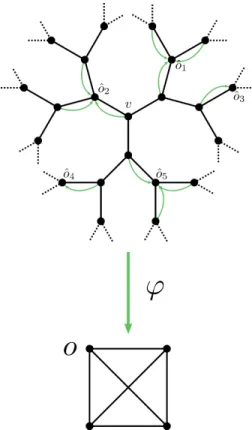
Letodenote a distinguished vertex ofG. Given a Td→Gcovering map ϕ, every vertex of
Figure 1. The case d= 3: ˆoi are the lifts of o∈V(K4); Xv is defined as Yoˆ2. Td is either a lift of o, or has a unique neighbor that is a lift of o (see Figure 1). Suppose that Y is an Aut(Td)-factor of IID on Td, and set
Xv ..=Yv0, wherev0 is the unique vertex such that ϕ(v0) =o and dist(v, v0)≤1.
It is easy to see that X = (Xv)v∈V(T
d) is a Γϕ-factor of IID and hence Corollary 2 can be applied to X. Given two neighboring vertices u and v in Td, the corresponding u0 and v0 either coincide (if ϕ(u) = o orϕ(v) =o), or they have distance 3. It follows that
H(µXe ) =
(H( ) if the edge e∈E(G) is incident to o, H( ) otherwise,
where represents two vertices of distance 3, and the notations H( ) and H( ) refer to entropies corresponding to the (Aut(Td)-factor of IID) process Y. Substituting these and H(µXv ) =H( ) into (4) we obtain, after cancellations, the following inequality for the process Y:
H( )≥
2− 2
d(d−1)
H( ).
This actually means that the normalized mutual information I(Yu;Yv)/H(Yv) is at most
2
d(d−1) for any verticesuand v of distance 3 inTd. The above argument can be generalized to obtain the following bounds for the normalized mutual information for arbitrary distance dist(u, v) =k. A different proof for this result can be found in an earlier paper [12] of the second and third author.
Theorem 3. [12, Theorem 1] Let d≥3 be an integer. For any u, v ∈V(Td) at distance k and for any Aut(Td)-factor of IID process Y on Td we have
(5) I(Yu;Yv)
H(Yv) ≤ ( 2
d(d−1)l if k = 2l+ 1 is odd,
1
(d−1)l if k = 2l is even.
Our general method is described in Section 3, it provides countless new entropy inequal- ities. We list a few examples in the rest of the introduction.
Let us fix an Aut(Td)-factor of IID process Y. Then for a finite set V ⊂ V(Td) the entropy of the joint distribution of Yv, v ∈ V, will be denoted by H(V). Because of the Aut(Td)-invariance of the process this joint distribution, and hence H(V), depends only on the “isomorphism type” of V in Td.
For instance, if V consists of the four vertices of a path of length three, then we do not need to specify where this path is in Td and we can simply write H( ) for H(V). The next theorem compares H( ) to H( ).
Theorem 4. The following path-edge inequality holds for any Aut(Td)-factor of IID pro- cess on Td:
H( )≥ 2d−3 d−1 H( ).
Another new inequality we obtain is
(6) H( d)≥(d−1)H( ).
The following two theorems generalize this inequality in different ways.
Theorem 5. Let Sk denote the set of vertices at distancek from a fixed vertex of Td. Then for any Aut(Td)-factor of IID process it holds that
(7) H(Sk)≥(d−1)kH( ).
Theorem 6. Let i denote the set ofi neighbors of a fixed vertex. Then for anyAut(Td)- factor of IID process and for any 1≤i < d it holds that
(d−i)H( i+ 1)≥(d−i−1)H( i) + (d−1)H( ), and hence by induction for any 1≤i≤d:
H( i)≥ id−2i+ 1
d−1 H( ), in particular, H( d)≥(d−1)H( ).
We will see in Section 4 that each of these inequalities is sharp in the sense that there are Aut(Td)-factors of IID processes for which the two sides of the inequality are asymptotically equal. We will also examine how strong our new inequalities are: it turns out that (6) and (7) are stronger than (1) and (2) for Markov chains indexed by Td.
Outline of the paper. The rest of the paper is structured as follows. In Section 2 we go through basic definitions and elaborate on the strength of Theorem 1 for different base graphs. In Section 3 we describe our general method for deriving new entropy inequalities from our general edge-vertex inequalities. In Section 4 we show that these new inequalities are sharp, and we compare them to previously-known ones. Finally, the proof of Theorem 1 is given in Section 5.
Acknowledgments. We are grateful to B´alint Vir´ag and M´at´e Vizer for fruitful discus- sions on the topic.
2. Preliminaries
2.1. Factors of IID. Suppose that a group Γ acts on a countable setS. Then Γ also acts on the spaceMS for a set M: for any functionf: S →M and for any γ ∈Γ let
(8) (γ·f)(s)..=f(γ−1·s) ∀s ∈S.
First we define the notion of factor maps.
Definition 2.1. LetM1, M2 be measurable spaces and S1, S2 countable sets with a group Γ acting on both. A measurable mapping F: M1S1 →M2S2 is said to be a Γ-factor if it is Γ-equivariant, that is, it commutes with the Γ-actions.
By aninvariant process onMS we mean an MS-valued random variable (or a collection of M-valued random variables) whose (joint) distribution is invariant under the Γ-action.
For example, ifZs, s∈S1, are independent and identically distributed M1-valued random variables, then we say that Z = (Zs)s∈S
1 is an IID process on M1S1. Given a Γ-factor F: M1S1 → M2S2, we say that X ..= F(Z) is a Γ-factor of the IID process Z. It can be regarded as a collection ofM2-valued random variables: X = (Xs)s∈S
2.
The results of this paper are concerned with factor of IID processes on infinite trees T: S1 andS2 are the vertex setV(T) and Γ is a subgroup of the automorphism group Aut(T).
The most important special case isT =Td and Γ = Aut(Td). When we say Γ-factor of IID process, we should also specify which IID process we have in mind (that is, specifyM1 and a probability distribution on it). By default we will work with the uniform distribution on [0,1]. In fact, as far as the class of Aut(Td)-factors is concerned, it does not really matter which IID process we consider. For example, for the uniform distribution on{0,1}we get the same class of factors as for the uniform distribution on [0,1]. This follows from the fact that these two IID processes are Aut(Td)-factors of each other [5].
The other important special case is when T is the universal cover of a finite connected simple graphGand Γ = Γϕ is the group of covering transformations for a coveringϕ: T → G. In this case it holds that for any ˆv1,vˆ2 ∈ V(T) with ϕ(ˆv1) = ϕ(ˆv2) there exists a unique γ ∈ Γϕ such that γ(ˆv1) = ˆv2. It follows that if we choose a fixed pre-image
¯
v ∈ ϕ−1(v) for every vertex v ∈V(G) of the base graph, then a Γϕ-factor F: [0,1]V(T) → MV(T) is determined by the functions f¯v ..= πv¯ ◦F: [0,1]V(T) → M, where πv¯ denotes the coordinate projection MV(T) → M corresponding to the vertex ¯v. Conversely, any collection of measurable functions fv¯: [0,1]V(T) → M, v ∈ V(G), gives rise to a Γϕ- factor mapping. (Note that an Aut(Td)-factor F is determined by a single function fo ..= πo◦F: [0,1]V(T) →M, but in that case fo needs to be invariant under all automorphisms of Td fixing the vertex o∈V(Td). See [1, Section 2.1] for details.)
2.2. Finite-radius factors. LetX be a Γ-factor of the IID processZ. We say thatX is a finite-radius factor (or ablock factor) if there exists a positive integerR such that for any vertexvthe value ofXv depends only on the valuesZufor verticesuin theR-neighborhood aroundv.
Can a factor of IID process be approximated by finite-radius factors? In many cases the answer is positive. This means that it suffices to prove certain statements for finite-radius factors. For instance, in the proof of Theorem 1 we will need the fact that an arbitrary Γϕ-factor of IID process is the weak limit of finite-radius Γϕ-factors. As we have seen, a Γϕ-factor F is determined by finitely many measurable [0,1]V(T) → M maps. The pre- image of an element m ∈ M under such a map is a measurable set in the product space [0,1]V(T), and, as such, it can be approximated by a finite union of measurable cylinder
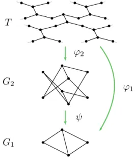
Figure 2. CoveringsT →G2 →G1
sets. Since M is finite in our case, it follows that any measurable [0,1]V(T)→M map can be approximated by maps for which all the pre-images are finite unions of cylinder sets, and consequently any Γϕ-factor can be approximated by finite-radius factors.
2.3. Finite coverings. Theorem 1 provides an inequality for any finite base graph G.
Next we elaborate on how these inequalities are related to each other.
Suppose thatG1 andG2 are finite connected (simple) graphs such that there is a covering map ψ: G2 → G1. Then the G2-version of Theorem 1 is stronger than the G1-version.
Indeed, let T denote their universal cover. Given a covering map ϕ2: T → G2, setting ϕ1 ..= ψ ◦ϕ2 yields a T → G1 covering map, see Figure 2. Clearly Γϕ2 ≤ Γϕ1. It follows that any Γϕ1-factor of IID process X onT is also Γϕ2-factor with the extra property that µXv (µXe ) depends only on the ψ-image of v ∈V(G2) (e ∈ E(G2)). Therefore it is easy to see that if we take theG2-version of the general edge-vertex inequality (3) and apply it to a Γϕ1-factor, we simply get back theG1-version of (3).
This means that one can get stronger and stronger versions of (3) by repeatedly lifting the finite base graph G.
2.4. Multiple edges and loops. A graph is calledsimple if it does not contain loops or multiple edges. For the sake of simplicity we stated (and we will prove) Theorem 1 for the case when the base graphG is simple. What can be said for base graphs that are not simple?
IfG has multiple edges (but no loops), then essentially the same result holds. The only difference is in the definition of a covering map T →G. In the case of simple graphs, one can simply say that a covering map is a mapping V(T)→ V(G) such that the neighbors of a vertex v are mapped bijectively to the neighbors of the image of v. When we have multiple edges, we also need to define the image of an edge: a covering map is a mapping V(T) → V(G) and a mapping E(T) → E(G) such that edges incident to a vertex v are mapped bijectively to edges incident to the image ofv. Once we know Theorem 1 for simple base graphs, it easily follows that it also holds when the base graphG has multiple edges:
simply take a finite simple graphG2 that covers G; then the G2-version of (3) implies the
G-version. (The proof of Theorem 1 presented in Section 5 would actually work for base graphs with multiple edges.)
As for loops the situation is a bit more complicated. In fact, one should distinguish between two kinds of loops. Loosely speaking: afull-loop can be travelled in two directions (contributing to the degree of the vertex by 2 and adding a free factorZto the fundamental group) while for a half-loop there is just one way of “going around” (contributing to the degree by only 1 and adding a free factorZ2 to the fundamental group). For our purposes the difference between them is how they behave under coverings. In short, an edge “double- covers” a half-loop while two parallel edges are needed to double-cover a full-loop. We should define covering maps rigorously for graphs containing full-loops, half-loops, multiple edges. Then this could lead to a version of (3) for arbitrary base graphs. The reason why we do not go into the details here is that, again, one can always take a finite simple lift of an arbitrary base graph and get a stronger version of the inequality.
If G has parallel edges (multiple edges between two vertices or more than one loops at one vertex), then we may choose not to “distinguish” some of those parallel edges but this would again lead to weaker inequalities. Note that in this terminology the original edge-vertex inequality (1) would correspond to the case when the base graph G consists of one vertex and d undistinguished half-loops, which is the weakest version of (4) in the d-regular case.
2.5. Connections to dynamical systems. These processes can be viewed in the context of ergodic theory. An invariant process (as defined in Section 2.1) gives rise to a dynamical system over Γ: the group Γ acts by measure-preserving transformations on the measurable spaceMS equipped with a probability measure (the distribution of the invariant process).
An IID process simply corresponds to a (generalized) Bernoulli shift. Therefore factor of IID processes are factors of Bernoulli shifts.
In fact, the general edge-vertex inequality (3) is related to a result of Lewis Bowen saying that the so-called f-invariant (for actions of the free group Fr) is non-negative for factors of the Bernoulli shift [8, Corollary 1.8]. This is essentially equivalent to Corollary 2 in the special case when the base graph G consists of one vertex andr =d/2 distinguished full-loops. See [12, Section 2.3] for details.
3. New inequalities for Aut(Td)-factors
In the introduction we already demonstrated on a simple example how Corollary 2 can be used to get new entropy inequalities for Aut(Td)-factors. In this section we describe our general method and present further examples.
Suppose thatY is an Aut(Td)-factor of IID process onMV(Td). Using the extra structure that a covering ϕ: Td → G gives, Y can be turned into a Γϕ-factor in many ways. For each v ∈ V(G) we fix a non-backtracking walk starting at v. Then for any lift ˆv ∈ V(Td) of v this walk can be lifted to get a path starting at ˆv. Let the endpoint of this path be assigned to ˆv. This assignment yields a mapping f: V(Td)→V(Td). It is easy to see that f is Γϕ-equivariant, and consequently Xu ..= Yf(u) defines a process X that is a Γϕ-factor of IID, and hence Corollary 2 can be applied to X. (The example in the introduction is the special case whenG=Kd+1, and for the distinguished vertexo ∈V(G) we choose the walk o of length 0, and for any other vertex v we choose the walk v →o of length 1.)
The general construction (where one can choose a finite collection of walks for each vertex) is described by the following lemma.
Lemma 3.1. Let G be a finite connected d-regular (simple) graph and ϕ: Td → G a covering map. Suppose that we have an Aut(Td)-factor of IID process Y on MV(Td). For any v ∈ V(G) let us choose a finite collection of (non-backtracking) walks on G (each starting at v): Wv,i, 1≤i≤kv.
For any liftvˆ∈V(Td)of v we lift eachWv,i starting atˆv. Then we consider the endpoints of these kv paths and Xˆv is defined to be the kv-tuple of theY-labels of these endpoints. It can be seen easily that the obtained processX is a Γϕ-factor of the IID process. (Note that the state space for X is M0 =M∪(M ×M)∪(M ×M ×M)∪. . .)
If we apply Corollary 2 to this process X, then we will get an inequality between the entropies of various finite subsets of V(Td) for the original Aut(Td)-factor of IID process Y. This works for any choice of a finite d-regular base graph G and walks Wv,i. In the remainder of this section we will show a few specific examples.
To keep our notations simple, in this section we will write µv and µe for µXv and µXe . Also,H( ) orH( ), and more generally H(V) for some V ⊂V(Td), will always refer to the entropy corresponding to the original Aut(Td)-factor process Y.
Two-vertex base graph, Theorem 4 and 6. As we discussed in Section 2.4 the general edge-vertex inequality is true even when the base graph G has multiple edges. So let G be the graph with two vertices (u and v) and d multiple edges e1, . . . , ed between them.
Given a positive integer i ≤ d−1 the following i walks (of length 1) are associated to u:
u−→e1 v;. . .;u−→ei v; while only the zero-length walk v is associated to v. Then H(µu) = H( i); H(µv) =H( ); H(µej) =
(H( i) if j ≤i, H( i+ 1) if j > i.
Substituting these into (4) we get the first inequality in Theorem 6. The second inequality follows easily by induction.
Next we consider the same base graph with different associated walks. Two walks starting at u, namely, uand u−→e1 v; and two walks starting atv, namely, v and v −→e1 u.
It is easy to see that H(µu) =H(µv) =H(µe1) =H( ), while for j ≥2 we have H(µej) = H( ), and consequently Theorem 4 follows from (4).
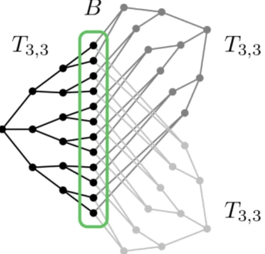
Sphere versus vertex, Theorem 5. For a setV ⊂V(Td) and a non-negative integerk letBk(V)..={u : dist(u, V)≤k}. Thek-ballBk({o}) around some rootowill be denoted byBk, whileSk ..=Bk\Bk−1 ={u : dist(o, u) = k} is the sphere of radiusk. Our goal is to get an inequality betweenH(Sk) and H( ).
We will need the following auxiliary graph to define our base graph: let Td,k denote a finite tree that is isomorphic to the subgraph of Td induced by the k-ball Bk. The vertex set ofTd,k can be partitioned into levels 0,1, . . . , k(based on the distance to the root), level i > 0 consisting ofd(d−1)i−1 vertices. All vertices have degree d except vertices at level k having degree 1. Any vertex at level 0< i < k is connected to one vertex at level i−1 and d−1 vertices at level i+ 1.
Now we take d copies of Td,k and “glue” them along their level-k vertices. This way we get a d-regular base graph G (essentially d balls of radius k with a shared boundary).
See Figure 3 for the case d = k = 3. The level-k vertices (that is, vertices on the shared boundary that we will denote by B) only get the zero-length walks. Any other vertex v belongs to exactly one copy ofTd,k. If we only use edges in this copy, then there is a unique
Figure 3. Three copies of T3,3 glued together along their boundary B path fromv to each vertex in B; let us associate these |B| paths tov. Then we have
H(µv) =
(H( ) if v ∈B,
H(Sk) if v /∈B; and H(µe) =H(Sk) for any e∈E(G).
Using (4) we get that
d|E(Td,k)|H(Sk)≥(d−1)|B|
| {z }
d(d−1)k
H( ) +d(d−1) (|V(Td,k)| − |B|)
| {z }
|E(Td,k)|−1
H(Sk),
and Theorem 5 follows.
Blow-ups. By a blow-up of an entropy inequality we mean the inequality we get if we replace each H(V) with H(Bk(V)) for a fixed positive integer k. It is not hard to show that if a linear entropy inequality is true for all Aut(Td)-factors of IID, then the blow-ups of this inequality are also true for all Aut(Td)-factors of IID.
For example, the blow-ups of the original edge-vertex inequality are:
(9) d
2H(Bk( )) ≥(d−1)H(Bk( )).
These blow-ups are closely related to Bowen’s definition of the f-invariant [7, 8]; in par- ticular, (9) follows from these papers.
There is a very short proof for (9) using our general method: one can take any base graph G and for each vertex take all non-backtracking random walks of length at most k. It is easy to see that every H(µv) equals H(Bk( )) and every H(µe) equals H(Bk( )), and hence we get (9). Moreover, if an inequality is attainable by our method, then so are its blow-ups: one needs to replace each associated walk in G with all walks obtained by concatenating this walk and any walk of length at most k.
We also mention that in [3] the blow-ups of the star-edge inequality (2) were proved for a broader class of invariant processes that were called typical processes. These blow-up inequalities played a central role in the proof of the main result of that paper. (Loosely speaking, a process is typical if it arises as a limit of labelings of randomd-regular graphs.
Their significance lies in the fact that many questions about random regular graphs can be studied through typical processes. It would be very interesting to know whether our new inequalities are also true for this broader class.)
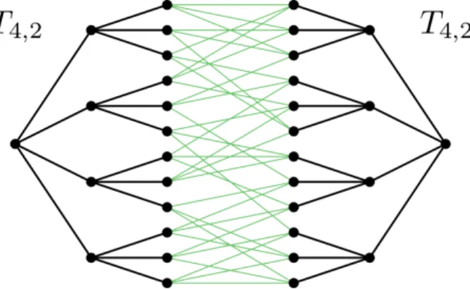
Figure 4. Two disjoint copies of T4,2 with additional edges between the boundaries Mutual information decay, Theorem 3. As we pointed out in the introduction, The- orem 3 was already proved in an earlier paper [12] of the second and third author. Next we show how this inequality follows easily from Corollary 2.
We need to define the base graphG slightly differently for odd and even k. For an odd distancek = 2l+ 1 let us take two copies of Td,l and add edges between their boundaries (that is, their level-l parts) in such a way that the obtained graph G is d-regular. Figure 4 shows the base graph for the case when d= 4;k = 5;l = 2.
As for the case whenk = 2l is even, one needs to connect the boundaries of a Td,l and a Td,l−1. Their boundaries are not of the same size, though, so we need to take d−1 copies of Td,l−1 and one copy of Td,l. Then we can add edges connecting the boundary vertices of Td,l to the boundary vertices of the copies of Td,l−1 in such a way that the obtained graph G isd-regular.
In both cases we have one walk associated to each vertex ofG: the unique path going to the root inside that copy. For allv ∈V(G) and for all original edgese(going inside a copy) we haveH(µv) =H(µe) =H( ). As for additional edgese (going between the boundaries of different copies), µe is the joint distribution of (Yu, Yv) for vertices u, v at distance k.
Substituting these into (4) leads to Theorem 3. The calculations are straightforward, we include the odd casek = 2l+ 1 here. Let B denote the boundary of Td,l; then
2|E(Td,l)|H( ) + (d−1)|B|H(Yu, Yv)≥2(d−1)|V(Td,l)|H( ).
Then for the mutual information I(Yu;Yv)..= 2H( )−H(Yu, Yv) we have (d−1)|B|
| {z }
d(d−1)l
I(Yu;Yv)
H( ) ≤2|E(Td,l)|+ 2(d−1)|B| −2(d−1)|V(Td,l)|= 2.
4. Sharpness, comparisons, applications
4.1. Sharpness. All the inequalities stated in this paper for Aut(Td)-factors (Theorem 3–6) are sharp in the following sense. Given a linear entropy inequality it is natural to normalize it by dividing both sides by the entropy of a vertex. We claim that there exist Aut(Td)-factor of IID processes for which the two sides of the inequality are arbitrarily close to each other (after normalization). In fact, for each inequality the same examples can be used to demonstrate the sharpness. These examples were already presented in [12]
to show that the upper bound for the normalized mutual information is sharp. For the sake of completeness we briefly recall these examples.
The idea is very simple: given IID labels at the vertices, let the factor process “list” all the labels within some large distanceR at any given vertex. One needs to be careful since listing the labels should be done in an Aut(Td)-invariant way. One possibility is to use the following lemma.
Lemma 4.1. [12, Lemma 5.2] For any positive integer L there exists a factor of IID coloring of the vertices of Td such that finitely many colors are used and vertices of the same color have distance greater than L.
Let us fix R and pick a very large L. Let C = (Cw)w∈V(T
d) be a factor of IID coloring provided by the lemma above. Given a positive integer N let Zw, w ∈ V(Td) be IID uniform labels from{1,2, . . . , N}. We set
Yv ={(Cw, Zw) | w∈BR(v)}.
Then Yv can be viewed as the list of variables (Cw, Zw), w ∈ BR(v), ordered by Cw (which are all different ifLis large enough). This is now an Aut(Td)-invariant description.
Furthermore, conditioned on the coloring process C the entropy corresponding to a finite subset V ⊂V(Td) is |BR(V)|log(N) provided that L is large enough. On the other hand, the contribution of the coloring to the entropies does not depend onN, so it gets negligible as N goes to infinity. One can easily check that if we replace H(V) by|BR(V)| in any of our inequalities, then the two sides will be asymptotically equal asR → ∞, and sharpness follows.
4.2. Hierarchy of entropy inequalities. We say that an entropy inequalityAisstronger than an inequality B (A⇒ B in notation) if the following is true: whenever an Aut(Td)- invariant processY (not necessarily factor of IID) satisfiesA, thenY also satisfiesB. There is a nested hierarchy between the blow-ups of the edge-vertex and star-edge inequalities:
· · · ⇒ d
2H(Bk+1( )) ≥(d−1)H(Bk+1( ))⇒H Bk( d)
≥ d
2H(Bk( ))
⇒ d
2H(Bk( ))≥(d−1)H(Bk( ))⇒ · · · In particular, the star-edge inequality (2) is stronger than the edge-vertex inequality (1), and, in turn, the blow-up (9) (fork = 1) of the edge-vertex inequality implies the star-edge inequality.
This can be seen using conditional entropies; we only include a sketch of the argument.
For finite sets U, W ⊂ V(Td) let H(W|U) denote the conditional entropy H(Yw, w ∈ W | Yu, u ∈ U). We will only use this in the special case when U ⊂ W, where we have H(W|U) = H(W)−H(U).
To see that (2) is stronger than (1): for any invariant processY satisfying (2) we have d
2H( )
(2)
≤ H( d) = H( ) +H( d| )≤H( ) + (d−1)H( | ) =dH( )−(d−1)H( ), and (1) follows.
A similar argument shows that for a process satisfying (9) (fork = 1) we have 2(d−1)
d H(B1( ))
| {z }
H( d) (9)
≤ H(B1( )) ≤H( d) +H( d| ) = 2H( d)−H( ),
and (2) follows.
Similar arguments were known by Bowen in the dynamical system context, see [7, Propo- sition 5.1].
4.3. Tree-indexed Markov chains. We have already seen that all our new entropy in- equalitites are sharp but the question remains: how strong are they compared to previously- known ones? Next we compare them for a specific class of processes.
An intriguing open problem about factor of IID processes is to determine the parameter regime where the Ising model on Td can be obtained as a factor of IID process. More generally, given a Markov chain indexed byTdwith some transition matrix, decide whether the corresponding invariant process is a factor of IID or not. (See [15, 2] and references therein.)
Here we focus on obtaining constraints for a Markov chain to be factor of IID. Two approaches have been used to show that a tree-indexed Markov chain cannot be factor of IID. The correlation bound given in [4] implies that the spectral radius of the transition matrix is at most 1/√
d−1 in the factor of IID case. The edge-vertex entropy inequality yields another constraint. For the Ising model the former gives a slightly better result.
There are examples, however, where the latter performs significantly better [2, Theorem 5].
One might think that the entropy approach can be improved by considering the stronger blow-up inequalities described above. However, for Markov chains all these blow-ups are equivalent to the edge-vertex inequality. This is due to the fact that for any connected subset V ⊂V(Td) we have
H(V) = H( ) + (|V| −1) H( | )
| {z }
H( )−H( )
= (|V| −1)H( )−(|V| −2)H( )
because of the Markov property. It follows that all known inequalities involving entropies of connected sets are equivalent to the edge-vertex inequality for tree-indexed Markov chains. In particular, H( d) ≥ (d−1)H( ), which follows by combining (1) and (2), is also equivalent to (1) for these processes.
We claim that our new entropy inequalities (7), proved in Theorem 5 for Aut(Td)-factors of IID, are stronger than (1) for tree-indexed Markov chains.
Proposition 4.2. For tree-indexed Markov chains the inequality H(Sk)≥(d−1)kH( ) is stronger than the edge-vertex inequality (1) and its blow-ups (9) for any given k.
Proof. The inequalityH(Sk)≥(d−1)kH( ) is clearly stronger than H(Bk)≥(d−1)kH( ).
The latter, however, is equivalent to (1) and (9) for tree-indexed Markov chains.
Therefore whenever the entropy approach performs better than the correlation bound, using Theorem 5 for any k≥1 instead of (1) will give an even better result.
As for which k we get the strongest inequality (for Markov chains), we do not have a complete answer. We can prove that fork = 2 the theorem is stronger than fork = 1, but we do not know if larger k always provides stronger inequality in Theorem 5.
5. Proof of the general edge-vertex inequality
To prove the original edge-vertex inequality (1) one needs to count colorings with given
“local statistics” on randomd-regular graphs [2, 16]. In order to obtain Theorem 1 we will generalize this argument for random lifts of a finite base graph G.
Let us fix a finite connected simple graph G and a covering map ϕ: T → G for the universal covering tree T. By Γ = Γϕ we denote the group of covering transformations of T. We will consider finite lifts ˆGof G and colorings of the vertices of ˆG.
Definition 5.1. Let ˆG be an N-fold lift of G. That is, we have a (deterministic) graph Gˆ and a covering ˆG→G such that every vertex/edge has exactly N lifts (i.e. pre-images under the covering map). Suppose that c: V( ˆG) → M is a (deterministic) coloring for some finite set M of colors.
By thelocal statisticsof the coloringcwe mean the following distributions: given a vertex v(or an edgee) ofG, letµcv (orµce) be the “empirical distribution” of the colors of theN lifts ofv (or e). More precisely, forv ∈V(G) let µcv be the distribution ofc(ˆv), where ˆv ∈V( ˆG) is chosen uniformly at random among the lifts ofv. Similarly, fore = (u, v)∈E(G) letµce denote the joint distribution of (c(ˆu), c(ˆv)), where ˆe = (ˆu,v)ˆ ∈ E( ˆG) is chosen uniformly at random among the lifts ofe.
Note that µce is a probability distribution on M ×M with the two marginals being µcu and µcv. Also, all the probabilities occuring in these distributions are multiples of 1/N.
From this point onε =ε(N) will denote a positive quantity that slowly converges to 0 asN → ∞. To be more specific, let ε =C/logN, whereC does not depend on N, but it might depend on the base graph G, the size of the state spaceM, and the radius R of the factor process. Note thatC might be different at each occurence ofε. The proof will have the following ingredients. (Some of the notions used here will be defined later.)
a) It holds with high probability that the random N-fold lift of a finite graphG has large essential girth, that is, the number of short cycles is small compared to the number of vertices.
b) Given any finite-radius Γ-factor of IID processX with finite state spaceM and a finite covering ˆG→Gthe following holds: there exists a deterministicM-coloring cof ˆGsuch that the local statistics µcv and µce are ε-close to µXv and µXe provided that the essential girth of ˆG is large enough.
c) Finally, we determine the expected number of M-colorings with given local statistics on a randomN-fold lift of G.
The general edge-vertex inequality (3) will follow easily by combining the above ingredients.
a) Random lifts. Given a finite simple base graph Gand a positive integerN, a random N-fold lift of G, denoted by ˆGN, is the following random graph: for each v ∈ V(G) we take N vertices Lv ..= {ˆv1, . . . ,ˆvN}, and for each e = (u, v) ∈ E(G) we take a uniform random perfect matching between Lu and Lv (independently for every edge e). Figure 5 shows such a random lift for a base graph with four vertices and five edges.
The above definition works for base graphs without loops. In this paper we do not need to use the notion of random lift for base graphs with loops. Let us note nevertheless that random d-regular graphs can be considered as random lifts of the graph with one vertex and d half-loops.
It is well known that a random N-fold lift has few short cycles. More precisely, [11, Lemma 2.1] shows that for any fixed positive integerl the expected number of l-cycles in a randomN-fold lift stays bounded as N → ∞. Using Markov’s inequality this immediately implies that with high probability the number of cycles of length at mostlis small compared to the number of vertices, which, in turn, implies that the random lift is locally a tree around most vertices. The exact statement we will use is the following.
Figure 5. The 4-fold random lift of a finite simple graph.
Lemma 5.2. Given any G and any positive integer R the random N-fold lift of Ghas the following property with probability 1−o(1) as N goes to infinity: the R-neighborhoods of all but at most εN edges are trees.
b) Projecting finite-radius factors onto large-girth graphs. The content of this section can be found in [16, Section 2.1] for the Aut(Td)-invariant case. The following is a straightforward adaptation for our setting.
Suppose that we have a finite-radius Γ-factor of IID process with radius R and let F: [0,1]V(T) → MV(T) be the corresponding Γ-factor mapping. (See Section 2.1 and 2.2 for definitions.) Next we explain how one can “project” such a process onto finite lifts of G.
Let ˆG be a fixed (deterministic) lift of G. We call a vertex/edge of ˆG R-nice if its R-neighborhood is a tree. By the type of a vertex ˆv ∈V( ˆG) we mean its image v ∈ V(G) under the covering map. Similarly, we can talk about the type of a vertex of the universal coverT.
Given an R-nice vertex ˆv ∈ V( ˆG) and an arbitrary vertex ¯v ∈ V(T) with the same typev ∈V(G), theirR-neighborhoods are clearly isomorphic. Moreover, there is a unique isomorphism between these neighborhoods that preserves the vertex types. In what follows we will use this unique isomorphism to identify these neighborhoods.
Now suppose that [0,1] labels are assigned to the vertices of ˆG. We will refer to these labels as input labels. Depending on these input labels we assign a state (i.e. an element fromM) to each vertex ˆv ∈V( ˆG), that is, we define a [0,1]V( ˆG)×V( ˆG)→M mapping. We pick an arbitrary fixed statem0 ∈M. If ˆv is notR-nice, we assignm0 to ˆv. If ˆv is R-nice, then we can “pretend” that we are at a vertex ¯v of the universal coverT: we copy the input labels onto the R-neighborhood of ¯v and apply the function f¯v ..=π¯v◦F: [0,1]V(T) →M; the value of fv¯ gets assigned to ˆv. (Recall that π¯v denotes the coordinate projection MV(T) →M corresponding to the vertex ¯v.)
For any Γ-factor process X with finite radius R and for any finite cover ˆG of G we described a mapping [0,1]V( ˆG)×V( ˆG)→M. If we choose the input labels randomly (IID and uniform [0,1]), then we get a random function c: V( ˆG) → M. We will think of c as a randomM-coloring of the vertices of ˆG that depends deterministically on the IID input labels. It is easy to see that this random coloring has the following properties.
• The distribution of the random color of anR-nice vertex of typev isµXv . Similarly, for an R-nice edge ˆe the joint distribution of the colors on the endpoints of ˆe is µXe for the corresponding e∈E(G). (See Theorem 1 for the definition ofµXv and µXe .)
• The color of a vertex depends only on the input labels in itsR-neighborhood. That is, if we change the labels outside its R-neighborhood, its color remains the same.
From now on we will assume that all but at most εN edges of ˆG are R-nice. Definition 5.1 defines the local statisticsµcv andµceof a deterministic coloringc: V( ˆG)→M. Here we have a random coloringc, thereforeµcvandµceare random measures depending on the input labels. Taking expectation (with respect to the input labels) we get the measuresEµcv and Eµce. We claim that Eµce is ε-close to µXe in total variation distance for each e ∈ E(G).
This follows from the fact that the color pair of anR-nice lift ofe has distributionµXe and that at mostεN edges are not R-nice among the N lifts of e.
Our goal is to show the existence of a deterministic coloring c: V( ˆG) → M with the property thatµceisε-close toµXe for eache∈E(G). At this point we have a random coloring for which this is true in expectation. We will use the following form of the Azuma–Hoeffding inequality to show that the local statistics of our random coloring are concentrated around their expectations.
Lemma 5.3. Let (Ωn, νn) be a product probability space. For a Lipschitz continuous func- tion f: Ωn →R with Lipschitz constant K (w.r.t. the Hamming distance on Ωn) we have (10) νn({ω∈Ωn : |f(ω)−Ef|> λ})≤2 exp
−λ2 2K2n
.
We use this in the following setting: Ω = [0,1], ν is the uniform measure on [0,1], and n = |V( ˆG)| = N|V(G)|. We will apply (10) to different functions f. Next we describe these functions.
Our random coloring c depends on the configuration ω ∈ Ωn ∼= [0,1]V( ˆG) of the input labels. For a given edge e = (v1, v2) ∈ E(G) and a given pair of colors m1, m2 ∈ M let f(ω) ..= N µce({(m1, m2)}), that is, f is the number of lifts of e = (v1, v2) with the first endpoint having color m1 and the second endpoint having color m2. Using the fact that the random color of a vertex depends only on the input labels in its R-neighborhood, it is easy to see that f is Lipschitz continuous with K = 2dR+1max, where dmax is the maximum degree of the base graph G.
Using (10) with λ = εN we get that the probability that µce({(m1, m2)}) is not ε-close to Eµce({(m1, m2)}) is very small: at most 2 exp(−ε2N). Recall that ε can denote any quantity C/logN whereC might depend on G, M, Rbut not on N.
Using union bound for alleand all pairs (m1, m2) we get that for large enoughN it holds with positive probability that µce is ε-close to Eµce for each e ∈ E(G). We have already seen that Eµce is ε-close toµXe , thus we have proved the following.
Lemma 5.4. Suppose that all but at most εN edges of Gˆ are R-nice and that N is large enough. Then there exists a deterministic coloring c: V( ˆG) → M such that µce is ε-close (say in total variation distance) to µXe for each edge e∈E(G).
c) The expected number of good colorings. Next we determine the expected number of colorings with prescribed local statistics on random lifts of a base graph. These local statistics need to be consistent in the following sense.
Definition 5.5. For a finite simple graph G and a finite color set M by a consistent collection of distributions we mean the following: a probability distribution µv on M for each v ∈ V(G) and a probability distribution µe on M ×M for each e ∈E(G) such that the marginals of µe for e= (u, v) are µu and µv.
Lemma 5.6. Let µv, v ∈ V(G), and µe, e ∈E(G), be a consistent collection of distribu- tions as in the definition above. Recall that GˆN denotes the random N-fold lift of G. Then the following formula holds for the expectation (w.r.t. GˆN) of the number of colorings on GˆN for which the edge-statistics coincide with µe:
(11) EGˆN
n
c: V( ˆGN)→M :µce =µe ∀e∈E(G) o
= exp
N
X
e∈E(G)
H(µe)− X
v∈V(G)
(degv−1)H(µv) +o(1)
as N → ∞
provided that the probabilities occuring in the discrete distributions µe are rational num- bers and N is a common multiple of all the denominators (otherwise the number of such colorings is clearly 0).
To prove the above lemma we will adapt the arguments in [2, Section 4] for our more general setting.
Given a discrete distributionµonM (set of colors) the multinomial coefficients describe the number of M-colorings of a finite set with color distribution µ. Using the Stirling formula it is easy to derive an asymptotic formula as the number of elements N goes to infinity: there are
exp (N(H(µ) +o(1)))
ways to choose the colors of N elements in a way that the number of elements with color m∈M isN µ({m}) (provided that these numbers are integers).
We will also need the following statement which is a slight variant of [2, Lemma 4.1].
Claim. Let Lu and Lv be disjoint sets of size N. Fix M-colorings of Lu and Lv with color distributions µu and µv, respectively. Let µe be any distribution on M×M with marginals µu and µv and with the property that all probabilities occuring in µe are multiples of 1/N. Then the probability that a uniform random perfect matching between Lu and Lv has color distribution µe is
(12) exp (N(H(µe)−H(µu)−H(µv) +o(1))).
(The color distribution of a matching is the distribution of the pair of colors on the end- points of the edges.)
Before proving this claim we show how Lemma 5.6 follows. First we take disjoint sets Lv of size N for each v ∈ V(G). Then we color each Lv with statistics µv. This can be done in
(13) exp
N
X
v∈V(G)
H(µv) +o(1)
different ways. Let us fix such a coloring c: ∪v∈V(G)Lv →M. To get a random lift of G we need to choose a uniform random perfect matching between Lu and Lv independently for each edge e = (u, v). The probability that this perfect matching has statistics µe (for any fixed coloring c) is given by the formula (12). These probabilities are independent and consequently the probability that a fixed coloring c is “good” for a random lift is the product of (12) with e running through E(G). To get the expected number of good colorings for a random lift we need to multiply this product by (13), and Lemma 5.6 follows.
Finally we prove the claim.
Proof of Claim. By a colored perfect matching between Lu and Lv we mean a coloring of the vertices inLu∪Lv and a perfect matching between Lu and Lv. There are two different ways to count the number of colored perfect matchings with color distributionµe:
(#all perfect matchings)·exp (N(H(µe) +o(1)))
= (#vertex colorings)
| {z }
exp(N(H(µu)+H(µv)+o(1)))
·(#good perfect matchings for any given vertex-coloring).
The claim immediately follows from this equality.
Putting the ingredients together. As we explained in Section 2.2, an arbitrary Γ-factor of IID processX is the weak limit of finite-radius factors. Since the entropies H(µXv ) and H(µXe ) are continuous under weak convergence, it suffices to prove Theorem 1 for finite- radius factors. So let us assume thatX is a Γ-factor of IID process with some finite radius R.
On a randomN-fold lift of Glet us consider the coloringscwith the property that µce is ε-close to µXe for all e∈E(G). We claim that the expected number of such colorings on a random lift is, on the one hand, at least 1−o(1), and, on the other hand, asymptotically equal to
(14) exp
N
X
e∈E(G)
H(µXe )− X
v∈V(G)
(degv−1)H(µXv ) +o(1)
as N → ∞.
Combining Lemma 5.2 and Lemma 5.4 implies that at least one such coloring exists for a random N-fold lift of G with probability 1−o(1). Therefore the expected number of such colorings is indeed at least 1−o(1).
To get (14) we need to apply Lemma 5.6 for all collections of distributionsµv andµewith the property that they areε-close toµXv andµXe , respectively, and that all the probabilities occuring are multiples of 1/N. It is easy to see that the total number of such collections is polynomial in N. We need to take the sum of (11) for all these collections. We can replace the entropiesH(µv) and H(µe) with H(µXv ) and H(µXe ) at the expense of ano(1) difference as N → ∞. We get (14) with an extra factor that is polynomial in N but that can be also incorporated in the N ·o(1) term in the exponent.
Therefore (14) is at least 1−o(1) asN → ∞ meaning that the term X
e∈E(G)
H(µXe )− X
v∈V(G)
(degv−1)H(µXv )
in the exponent cannot be negative, and this is exactly what we wanted to prove.
![arXiv:1707.05064v3 [math.PR] 21 Mar 2019](data:image/gif;base64,R0lGODlhAQABAIAAAP///wAAACH5BAEAAAAALAAAAAABAAEAAAICRAEAOw==)