Newmethodsincomputeraidedmodelingofcurvesandsurfaces MiklósHoffmann

Eszterházy Károly College

Institute of Mathematics and Computer Science

Miklós Hoffmann

New methods in computer aided modeling of curves and surfaces

Eger, 2014

1.3.1 B-spline curve passing through a point . . . 17

1.3.2 NURBS curve passing through a point . . . 19

1.3.3 Modification of two weights and a knot value of a NURBS curve . . . 20

1.3.4 Further constrained modification tools by knots . . . 20

1.4 Extension to surfaces . . . 29

2 New curve types in geometric modeling 31 2.1 Linear blending of curves - the quartic curve of Han . . . 31

2.1.1 Definition and linear blending description . . . 32

2.1.2 Linear blending on a common basis . . . 33

2.1.3 Shape parameter alteration . . . 35

2.1.4 Constrained shape modification . . . 38

2.2 C-curves . . . 38

2.2.1 Paths of C-Bézier curves and their extensions . . . 39

2.2.2 Paths of C-B-spline curves and their approximate lines . . . 41

2.3 FB-spline curves . . . 43

2.3.1 Control point based methods . . . 45

2.3.2 Shape parameter based methods . . . 47

2.4 A trigonometric curve with exponential shape parameters . . . 50

2.4.1 New basis functions . . . 51

2.4.2 Nonnegativity . . . 52

2.4.3 Linear independence . . . 55

2.4.4 The curve . . . 62

3 Non-control-point-based methods 65 3.1 Modeling unorganized points by artificial neural networks . . . 65

3.1.1 The Kohonen neural network and its application . . . 66

3.1.2 Numerical control of the training: the gain term and the neighborhood function . . . 70

3.1.3 Ruled surfaces from a set of rulings . . . 72

3.2 Sphere-based modeling . . . 73

3.2.1 Previous work . . . 76

3.2.2 Skinning of circles . . . 78

3.2.3 Extension to spheres . . . 83

3.2.4 Surfaces with multiple branches . . . 87

3.2.5 Results and comparison with other methods . . . 92

Bibliography 96

61]. The last chapter provides an overview on non-control-point-based methods, based on the results published in [2,32,33,36,38,69,110].

Here I would like to thank my distinguished colleagues and co-authors for the inspiring atmosphere of our scientific discussions. This dissertation would not have been possible without their help.

1 Knots of B-spline and NURBS curves and surfaces

1.1 Basic definitions

B-spline and NURBS curves are standard description methods and hence widely used in com- puter aided design today. There are several books and papers on these curves describing their properties, with the help of which one can apply them as powerful design tools. The basic definitions (as one can find e.g. in [90]) are the following:

Definition 1.1. The recursive functionN_j^k given by the equations

N_j¹(u) = (

1 ifu∈[u_j, u_j+1), 0 otherwise

N_j^k(u) = _u ^u−uj

j+k−1−ujN_j^k−1(u) +_u^uj+k−u

j+k−uj+1N_j+1^k−1(u)

is called normalized B-spline basis function of orderk(degreek−1). The numbersu_j ≤u_j+1∈R are called knot values or simply knots, where 0/0 ˙=0 by definition.

Definition 1.2. The curve s(u) defined by s(u) =

Xn

l=0

d_lN_l^k(u), u∈[u_k−1, u_n+1]

is called B-spline curve of order k (degree k−1), where N_l^k(u) is the l^th normalized B-spline basis function, for the evaluation of which the knots u₀, u₁, . . . , u_n+k are necessary. The points d_i are called control points or de Boor-points, while the polygon formed by these points is called control polygon. The arcs of this B-spline curve are called spans. The j^th span can be written as

s_j(u) = Xj

l=j−k+1

d_lN_l^k(u), u∈[u_j, u_j+1).

As one can observe from the definitions above, B-spline curve is uniquely defined by its degree, control points and knot values, while in terms of NURBS curves the weight vector has to be specified in addition. It is an obvious fact that the modification of each of these data will affect the shape of the curve and some of its geometric properties. The modification of a curve plays central role in CAD systems, hence numerous methods are presented to control the shape of a curve by modifying one of its data mentioned above. The most basic possibilities can be found in any book of the field. Further control point-based shape modification is discussed in [88] and [26], weight-based modification is described e.g. in [88] and [55], while others present shape control by simultaneous modification of control points and weights (see [1], [101]).

The effect of a change of the knot vector on the shape of the curve, however, has not been described yet. Even in one of the most comprehensive books ([90]) one can read the following:

"Although knot locations also affect shape, we know of no geometrically intuitive or mathemati- cally simple interpretation of this effect...". The aim of this section is to present the geometrical and mathematical representation of the effects of knot modification for B-spline curves and sur- faces, based on the contributions of Hoffmann and Juhász, presented in [35,37,40,57,58,59,60].

4. The modification of the knotu_i affects only the functionsN_i−k^k (u), . . . , N_i^k(u), hence only the shape of the spans s_i−k+1(u), . . . ,s_i(u), . . . ,s_i+k−2(u) of the curve will be changed.

1.2 Geometric effects of the modification of a knot

When modifying the knotu_i, the basis functions and spans described in Property 4will depend not only on u but onu_i as well. To emphasize this fact, they will be denoted by N_i^k(u, u_i)and s_i(u, u_i). Fixing the second one of the two variables (i.e. the knot valueu_i= ˜u_i) one can receive the original basis functions N_i^k(u,u˜_i) =N_i^k(u) and spans s_i(u,u˜_i) = s_i(u), but fixing the first variable (i.e. the parameter u= ˜u) the functions N_i^k(˜u, u_i) will not remain the standard basis functions any more, but some rational functions of u_i, while s_i(˜u, u_i) can be interpreted as a curve on which a point of the original B-spline moves. More precisely, when modifying the knot u_i the point of the spans_j(u)associated with the fixed parameter valueu˜∈[u_j, u_j+1)will move along the curve

s_j(˜u, u_i) = Xj

l=j−k+1

d_lN_l^k(˜u, u_i), u_i∈[u_i−1, u_i+1].

Hereafter, we refer to this curve as the path of the points_j(˜u). At the first part of this section these functions and paths will be examined, especially in terms of their degree.

Lemma 1.3. N_i−k^k (˜u, u_i),u˜∈[u_i−m, u_i−m+1),(m= 1, . . . , k−1),u_i ∈[u_i−1, u_i+1]is a rational function of degree k−m in u_i.

Proof. In the recursive Definition1.1 N_i−k^k (˜u, u_i) = u˜−u_i−k

u_i−1−u_i−kN_i−k^k−1(˜u, u_i) + u_i−u˜

u_i−u_i−k+1N_i−k+1^k−1 (˜u, u_i)

the first term is independent ofu_i because of Property 4, hence only the second term has to be considered. This fact is also valid for the further steps of the recursion:

...

N_i−m−1^m+1 (˜u, u_i) = u˜−u_i−m−1

u_i−1−u_i−m−1N_i−m−1^m (˜u, u_i) + u_i−u˜

u_i−u_i−mN_i−m^m (˜u, u_i) N_i−m^m (˜u, u_i) = u˜−u_i−m

u_i−1−u_i−mN_i−m^m−1(˜u, u_i) + u_i−u˜

u_i−u_i−m+1N_i−m+1^m−1 (˜u, u_i).

The first term of the right hand side of both equations above is constant because of Property4.

The second term of the last equation is equal to 0 due to Property1. Thus u_i appears only in k−m terms, at degree1 everywhere, consequently, the degree of the functionN_i−k^k (˜u, u_i) inu_i is k−m.

Theorem 1.4. The path s_i−m(˜u, u_i) = ^i−mP

l=i−m−k+1

N_l^k(˜u, u_i)d_l, u_i ∈ [u_i−1, u_i+1] is a rational curve of degree k−m with respect tou_i, ∀˜u∈[u_i−m, u_i−m+1),(m= 1, . . . , k−1).

Proof. The lower limit of the summation can be increased to i−k, since u_i has no effect on N_l^k(˜u, u_i) for l < i−k (see Property4). Hence only the functions

N_i−k+z^k (˜u, u_i), z= 0, . . . , k−m (1.1)

have to be considered. The functionN_i−k^k (˜u, u_i)is of degreek−mbecause of Lemma1.3. Thus it is sufficient to prove that the degree of the functions (1.1) is at most k−m, for z >0.

At ther^th step of the recursion those functions which have influence on the functions men- tioned above can be described in the following form (see Property2):

N_i−k+z+n^k−r (˜u, u_i) = u˜−u_i−k+z+n

u_{i+z+n−r−1}−u_i−k+z+nN_i−k+z+n^k−r−1 (˜u, u_i) + u_i+z+n−r−u˜

u_i+z+n−r−u_i−k+z+n+1N_i−k+z+n+1^k−r−1 (˜u, u_i) r = 0, . . . , k−1;n= 0, . . . , r.

In this form u_i can occur in the following cases:

1. i−k+z+n= i, i.e. z+n−k = 0, that is the function N_i^k−r−1(˜u, u_i) appears in the first term, but this function is equal to0 on the interval[u_i−m, u_i−m+1)for all permissible values ofm (see Property1).

2. i+z+n−r−1 =i, that isz+n=r+ 1, hence the normalized B-spline basis function in the first term is N_{i−(k−r−1)}^k−r−1 (˜u, u_i). According to Lemma 1.3, the degree of this function in u_i isk−m−r−1, hence the degree of the first term can at most bek−m−r ≤k−m.

3. i+z+n−r=i, that is z+n=r, which corresponds to case 2.

4. i−k+z+n+ 1 =i, which corresponds to case 1.

Corollary 1.5. For m = k−1, the resulted path is of degree 1, that is if u_i runs from u_i−1 to u_i+1, then the points of the span s_i−k+1(˜u, u_i) move along straight lines parallel to the side d_i−k,d_i−k+1 of the control polygon.

In this case the path has the following simple form:

s_i−k+1(˜u, u_i) =N_i−k^k (˜u, u_i)d_i−k+N_i−k+1^k (˜u, u_i)d_i−k+1,

s_i−k+1(˜u, u_i) = µ

C₁(˜u) +C₂(˜u) µ

1− u˜−u_i−k+1 u_i−u_i−k+1

¶¶

d_i−k+C₂(˜u) u˜−u_i−k+1

u_i−u_i−k+1d_i−k+1

= (C₁(˜u) +C₂(˜u))d_i−k+C₂(˜u) u˜−u_i−k+1

u_i−u_i−k+1 (d_i−k+1−d_i−k).

Until now the movement of those points and parts of the B-spline curve was clarified, the parameters of which are smaller than the knot value u_i subject to change. Similar statements hold for those parts of the B-spline curve, which correspond to the parameter values succeeding the knot u_i.

Lemma 1.6. The function N_i^k(˜u, u_i), u˜∈[u_i+m, u_i+m+1), (m= 0, . . . , k−2), u_i∈[u_i−1, u_i+1] is a rational function of degree k−m−1 in u_i.

Proof. The proof of this lemma is analogous to that of Lemma1.3.

Theorem 1.7. The path s_i+m(˜u, u_i) = ^i+mP

l=i+m−k+1

N_l^k(˜u, u_i)d_l, u_i ∈ [u_i−1, u_i+1] is a rational curve of degree k−m−1 with respect to u_i, ∀˜u∈[u_i+m, u_i+m+1), (m= 0, . . . , k−2).

Proof. The upper limit of the summation can be decreased to i, since u_i has no influence on N_l^k(˜u, u_i) for l > i (see Property 4). By using Lemma 1.6, the further part of the proof is analogous to that of Theorem 1.4.

Corollary 1.8. Form=k−2, the path is of degree 1, that is ifu_i runs from u_i−1 tou_i+1 then the points of the span s_i+k−2(˜u, u_i) move along straight lines parallel to the side d_i−1,d_i of the control polygon.

Now we can summarize our results based on Theorem 1.4 and 1.7 and their corollaries.

Modifying the knot value u_i the points of the spans of a k^th order B-spline curve move along rational curves, the degree of which decreases symmetrically from k−1 to 1 as the indices of the spans getting farther from i. Hence the points of the spanss_i−k+1(˜u, u_i) and s_i+k−2(˜u, u_i) move along straight lines parallel to the corresponding sides of the control polygon. Other parts of the curve remain unchanged (see Figure1.2).

Figure 1.1. Paths of the points of a cubic B-spline curve when ui runs from ui−1 to ui+1 and the two extreme positions of the curve: ui =ui−1 (solid line) and ui =

ui+1(dashed line)

1.2.1 The envelope of the family of B-spline curves

The modification of a knot value u_i results a one-parameter family of B-spline curves s(u, u_i) =

Xn

l=0

d_lN_l^k(u, u_i), u∈[u_k−1, u_n+1], u_i ∈[u_i−1, u_i+1). (1.2) In case of k = 3 the spans of the curves are parabolic arcs. It is well-known that the tangent lines of these arcs at the knot values coincide with the sides of the control polygon. Modifying a knot value u_i the tangent line remains the same, which can be interpreted as the side of the control polygon is the envelope of the family of these quadratic B-spline curves. In the following theorem the generalization of this property will be proved for arbitrary degree k.

Theorem 1.9. The family of the k^th order B-spline curves s(u, u_i) = Pⁿ

l=0

d_lN_l^k(u, u_i), u ∈ [u_k−1, u_n+1],u_i∈[u_i−1, u_i+1), k >2has an envelope. This envelope is a B-spline curve of order (k−1)and can be written in the form

b(v) = Xi−1

l=i−k+1

d_lN_l^k−1(v), v∈[v_i−1, v_i], (1.3)

l=i−k+1

the starting point of which is s(u_i, u_i)can be written in the form s_i(u, u_i) =

Xi

l=i−k+1

d_l

µ u−u_l

u_l+k−1−u_lN_l^k−1(u) + u_l+k−u

u_l+k−u_l+1N_l+1^k−1(u)

¶

. (1.5)

At the specific parameteru_i the value of this function is s_i(u_i, u_i) =

Xi−1

l=i−k+1

d_l

µ u_i−u_l

u_l+k−1−u_lN_l^k−1(u_i) + u_l+k−u_i

u_l+k−u_l+1N_l+1^k−1(u_i)

¶

(1.6)

(the upper limit of the summation can be decreased to i−1, since N_i^k−1(u_i) =N_i+1^k−1(u_i) = 0).

Now we insert the knot valueu_i between v_i−1 andv_i (v_i−1 =u_i−1 ≤u_i ≤u_i+1 =v_i) by the Böhm’s insertion algorithm (cf. [8]). The new knot vector is

ˆ v_j =







v_j =u_j if j < i

u_i if j =i

v_j−1 =u_j if j > i

(1.7)

For the normalized B-spline basis functionsN_l^k−1(v)andNˆ_l^k−1(v), defined over the knot vectors (v_j) and (ˆv_j) respectively, the following relation holds:

N_l^k−1(v) =

















Nˆ_l^k−1(v) if l < i−k+ 1;

ui−ˆvl

ˆ

vl+k−1−ˆvl

Nˆ_l^k−1(v) +_vˆ^vˆl+k−ui

l+k−ˆvl+1

Nˆ_l+1^k−1(v) if l=i−k+ 1, . . . , i−1;

Nˆ_l+1^k−1(v) if l > i−1.

Based on this fact the following form can be obtained b(v) = ⁱ⁻¹P

l=i−k+1

d_l

³ ui−ˆvl

ˆ

vl+k−1−ˆvl

Nˆ_l^k−1(v) +_ˆv^ˆvl+k−ui

l+k−ˆvl+1

Nˆ_l+1^k−1(v)

´

v ∈[ˆv_i−1,vˆ_i+1)

and using (1.7) this can be written in the form (sinceˆv_j =u_j,∀j) b(u) = ⁱ⁻¹P

l=i−k+1

d_l

³ ui−ul

ul+k−1−ulN_l^k−1(u) +_u^ul+k−ui

l+k−ul+1N_l+1^k−1(u)

´

u∈[u_i−1, u_i+1).

(1.8)

Comparing (1.6) and (1.8) one can see thatb(u_i) =s_i(u_i, u_i) holds.

The derivative of the curve (1.8) with respect tou is b˙(u) =

Xi−1

l=i−k+1

d_l

µ u_i−u_l

u_l+k−1−u_lN˙_l^k−1(u) + u_l+k−u_i

u_l+k−u_l+1N˙_l+1^k−1(u)

¶

. (1.9)

Based on (1.4), the derivative of the curves_i(u, u_i) with respect to u is

˙

s_i(u, u_i) = Xi

l=i−k+1

d_lN˙_l^k(u, u_i), (1.10) while on the other hand, using (1.5)

˙

s_i(u, u_i) =

Xi

l=i−k+1

d_l

³ 1

ul+k−1−ulN_l^k−1(u)−_u ¹

l+k−ul+1N_l+1^k−1(u) +

u−ul

ul+k−1−ul

N˙_l^k−1(u) +_u^ul+k−u

l+k−ul+1

N˙_l+1^k−1(u)

´

holds. Applying Property3, this can be written as s˙_i(u, u_i) = Pⁱ

l=i−k+1

d_l

³ u−ul

ul+k−1−ul

N˙_l^k−1(u) +_u^ul+k−u

l+k−ul+1

N˙_l+1^k−1(u) +

k−11 N˙_l^k(u)

´ .

(1.11)

Based on (1.10) and (1.11) one can write u−u_l

u_l+k−1−u_lN˙_l^k−1(u) + u_l+k−u

u_l+k−u_l+1N˙_l+1^k−1(u) = k−2

k−1N˙_l^k(u). Hence from (1.10) and (1.9) we obtain

b˙(u_i) = k−2

k−1s˙_i(u_i, u_i).

The envelope is illustrated by Figure 2.

1.2.2 The envelope of the paths of curve points

Two families of curves have been considered so far, the paths of the points and the family of B-spline curves themselves. These two families of curves can be considered as parameter lines of

Figure 1.2. Envelope of the family of cubic B-spline curves whenuiruns fromui−1 toui+1

the surface patch

s(u, u_i) = Xn

l=0

d_lN_l^k(u, u_i), u∈[u_k−1, u_n+1], u_i ∈[u_i−1, u_i+1).

The envelope mentioned above in Theorem1.9is a curve on this surface, but the parameter lines behave in a singular way at the points of that curve. We have seen that it is an envelope of the family of B-spline curves. In the next subsection, where we will restrict our consideration to the cubic case (k = 4) we will prove, that this curve is also the envelope of the paths and both families have the same osculating plane at every point of this envelope, which plane is also the plane of the envelope itself (c.f. [34]).

Theorem 1.10. If we consider the surface s_i(u, u_i), u∈ [u_k−1, u_n+1], u_i ∈[u_i−1, u_i+1) then the envelope of the family of B-spline curves s_i(u,u˜_i) is also the envelope of the family of paths s_i(˜u, u_i) at the points corresponding to u=u_i.

Proof. It is sufficient to prove, that the two families of curves have points and tangent lines on common at the points corresponding to the parameter value u = u_i. If we fix the parameters u = ˜u and u_i = ˜u_i then a member of both families of curves has been selected. Substituting these parameters to both of the curves the existence of the common point s_i(˜u,u˜_i) =s_i(˜u,u˜_i) immediately follows. For the proof of the common tangent lines the first derivatives of these curves will be used. Substituting the parameteru=u_ito the coefficients after some calculations

one can receive, that

∂N_i−3⁴

∂ui

¯¯

¯u=ui

= −¹₃^∂N_∂uⁱ⁻³⁴

¯¯

¯u=ui

= _ui+1−u¹ _i−2u^u_i+1ⁱ⁺¹_−u^−u_i−1ⁱ

∂N_i−2⁴

∂ui

¯¯

¯u=ui

= −¹₃^∂N_∂uⁱ⁻²⁴

¯¯

¯u=ui

= _u ¹

i+1−ui−1

³ ui−ui−2

ui+1−ui−2 −_u^ui+2−ui

i+2−ui−1

´

∂N_i−1⁴

∂ui

¯¯

¯u=ui

= −¹₃^∂N_∂uⁱ⁻¹⁴

¯¯

¯u=ui

= −_u ¹

i+1−ui−1

ui−ui−1

ui+2−ui−1

∂N_i⁴

∂ui

¯¯

¯u=ui

= ^∂N_∂uⁱ⁴

¯¯

¯u=ui

= 0

which yields, that

∂s_i(u, u_i)

∂u

¯¯

¯¯

u=ui

=−1 3

∂s_i(u, u_i)

∂u_i

¯¯

¯¯

u=ui

i.e. the curves have also tangent lines in common at the points of the envelope.

With the help of the second derivatives of the coefficient functions the osculating plane of these curves can also be examined.

Theorem 1.11. The osculating planes of the two families of curves s_i(u,u˜_i)ands_i(˜u, u_i) coin- cide at every point of the envelope and this plane is that of the three control pointsd_i−3,d_i−2,d_i−1 for every u_i.

Proof. The osculating plane is uniquely defined by the first and second derivatives of the curve.

Since Theorem 3. holds for the first derivatives it is sufficient to prove that the second derivatives of these curves are also parallel to each other. Using the second derivatives of the coefficient functions and substituting the parameter valueu=u_i the following result can be obtained:

∂²N_i−3⁴

∂ui2

¯¯

¯u=ui

= ¹₃^∂2_∂u^Ni−342

¯¯

¯u=ui

= 2_u ¹

i+1−ui−2

ui+1−u1 i−1

∂²N_i−2⁴

∂ui2

¯¯

¯u=ui

= ¹₃^∂2_∂u^Ni−242

¯¯

¯u=ui

= 2_(−u ^{−ui+1+ui−2−ui+2+ui−1}

i+2+ui−1)(ui+1−ui−1)(−ui+1+ui−2)

∂²N_i−1⁴

∂ui2

¯¯

¯u=ui

= ¹₃^∂2_∂u^Ni−142

¯¯

¯u=ui

= 2_(u ¹

i+1−ui−1)(ui+2−ui−1)

∂²N_i⁴

∂ui2

¯¯

¯u=ui

= ^∂_∂u^2N2ⁱ⁴

¯¯

¯u=ui

= 0

which immediately yields, that

∂²s_i(u, u_i)

∂u²

¯¯

¯¯

u=ui

= 1 3

∂²s_i(u, u_i)

∂u_i²

¯¯

¯¯

u=ui

.

Hence the osculating planes of the two families of curves coincide at the parameter valuesu=u_i. Moreover, the second derivatives do no depend on u_i, and using the notations

A:= ∂²N_i−3⁴

∂u_i² , B := ∂²N_i−1⁴

∂u_i² they can be written in the form

∂²si(u,ui)

∂ui2

¯¯

¯u=ui

= A(d_i−3−d_i−2) +B(d_i−2−d_i−1)

∂²si(u,ui)

∂u²

¯¯

¯u=ui

= ¹₃A(d_i−3−d_i−2) +¹₃B(d_i−2−d_i−1).

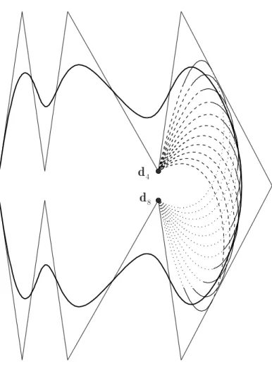
u_i−1 and larger than u_i+1. For these extended paths the following holds.

Theorem 1.12. Modifying the single multiplicity knot u_i of the B-spline curve s(u), points of the extended paths of the arcs s_i−1(u) and s_i(u) tend to the control points d_i and d_i−k as u_i tends to −∞and ∞, respectively, i.e.,

uilim→−∞s(u, u_i) =d_i, lim

ui→∞s(u, u_i) =d_i−k,∀u∈[u_i−1, u_i+1).

Proof. We prove the statement for the arcs_i(u), fors_i−1(u)it can be proved analogously. Denote the original knot values by u¯_j, (j = 0,1, . . . , n+k). For the description of extended paths we will use the knot values u_j = ¯u_j,(j = 0,1, . . . , n+k) which will differ from the original values only in u_i along the proof. Paths of the points s_i(u) can be written as

s_i(u, u_i) = Xi

l=i−k+1

d_lN_l^k(u, u_i), u_i∈[¯u_i−1,u¯_i+1), u∈[¯u_i,u¯_i+1]. (1.12)

Limits of this summation are modified when we extend these paths, since if u_i > u¯_i+1 (i.e., u_i → ∞) then N_i^k(u) ≡0, u∈[¯u_i,u¯_i+1] and N_i−k^k (u) 6= 0, u∈ [¯u_i,u¯_i+1], thus these arcs of the extended paths become

s_i(u, u_i) = Xi−1

l=i−k

d_lN_l^k(u, u_i), u_i >u¯_i+1, u∈[¯u_i,u¯_i+1]. It can easily be seen that

N_i−k^k (u, u_i) = (u_i−u)^k−1

k−1Q

j=1

(u_i−u_i−j)

where both the numerator and the denominator are polynomials of degree k−1 inu_i, and the main coefficient in both polynomials is 1. This yields lim

ui→∞N_i−k^k (u, u_i) = 1. Now we prove by induction onk that lim

ui→∞N_j^k(u, u_i) = 0,(j=i−k+ 1, . . . , i−1).

i) for k= 3

N_i−1³ (u, u_i) = (u−u_i−1)²

(u_i+1−u_i−1) (u_i−u_i−1),

N_i−2³ (u, u_i) = (u−u_i−2) (u_i−u)

(u_i−u_i−2) (u_i−u_i−1)+ (u_i+1−u) (u−u_i−1) (u_i+1−u_i−1) (u_i−u_i−1) for which the statement holds.

ii) k−1→k

By Definition1.1

N_i−1^k (u, u_i) = u−u_i−1

u_i+k−2−u_i−1N_i−1^k−1(u, u_i) + u_i+k−1−u

u_i+k−1−u_iN_i^k−1(u, u_i) N_i−2^k (u, u_i) = u−u_i−2

u_i+k−3−u_i−2N_i−2^k−1(u, u_i) + u_i+k−2−u

u_i+k−2−u_i−1N_i−1^k−1(u, u_i) ...

N_i−k+1^k (u, u_i) = u−u_i−k+1

u_i−u_i−k+1N_i−k+1^k−1 (u, u_i) + u_i+1−u

u_i+1−u_i−k+2N_i−k+2^k−1 (u, u_i)

Therefore, the k^th order functions are linear combinations of functions of orderk−1 where the numerator is independent of u_i and the denominator is linear at most in u_i, i.e., the order of the numerator can not be greater than that of the denominator. Thus, from the assumption for k−1, the case ofk results too.

Ifu_i <u¯_i−1 (u_i→ −∞) then the limits of the summation (1.12) are not modified. It is easy to show that in this case

N_i^k(u, u_i) = (u−u_i)^k−1

k−1Q

j=1

(u_i+j−u_i) which immediately yields lim

ui→−∞N_i^k(u, u_i) = 1.

Equalities lim

ui→−∞N_i−j^k (u, u_i) = 0,(j = 1,. . .,k−1)can be proved by induction on k.

This property of the extended paths is illustrated in Fig. 1.3.

It is easy to show that, by altering a knot of higher multiplicity, Theorem1.12will be of the following form.

Theorem 1.13. Altering the knotu_i of multiplicity m, points of the extended paths of the arcs s_i−1(u),. . ., s_i+m−1(u) satisfy the equalities

ui→−∞lim s_i+j(u, u_i) =d_i+m−1, lim

ui→∞s_i+j(u, u_i) =d_i−k, (j=−1,0, . . . , m−1),∀u∈[u_i+j, u_i+j+1).

1.2.4 The case of higher order contact and higher multiplicity of knots

Theorem1.9can be generalized in two ways. At first we prove that the family of B-spline curves (1.2) and the envelope curve (1.3) have higher derivatives in common. Then we will consider the case when the modified knot is of multiplicitym >1.

Figure 1.3. A cubic B-spline curve and its extended paths (n= 12, k= 4, i= 8).

Theorem 1.14. Let us consider the one-parameter family of B-spline curves of order k s(u, u_i) =

Xn

l=0

d_lN_l^k(u, u_i), u∈[u_k−1, u_n+1], u_i ∈[u_i−1, u_i+1), k >2

obtained by the modification of the knot u_i of single multiplicity between its neighboring knots.

Also consider the B-spline curve

b(v) = Xi−1

l=i−k+1

d_lN_l^k−1(v), v∈[v_i−1, v_i]

of order k−1 defined by the same control pointsd_l, and the knotsv_j =u_j ifj < iandv_j =u_j+1 otherwise, i.e., we leave out the knotu_i from the knot vector{u_j}. Then the relation between the derivatives of these two curves at u=v=u_i is

d^r dv^rb(v)

¯¯

¯v=ui

= k−1−r k−1

d^r

du^rs(u, u_i)

¯¯

¯u=ui

, r≥0.

Proof. The proof follows the basic idea of the proof of Theorem1.9where we proved the statement for the caser= 1. To make the two curves compatible, we insert the knotu_iinto the knot vector

{v_j}with Boehm’s insertion algorithm [8]. After the conversion of knots from{v_j} to{u_j}, this yields the new representation

b(u) = Xi−1

l=i−k+1

d_l

µ u_i−u_l

u_l+k−1−u_lN_l^k−1(u) + u_l+k−u_i

u_l+k−u_l+1N_l+1^k−1(u)

¶

, u∈[u_i−1, u_i+1) (1.13)

of curve (2.6). It is easy to show that b(u_i) =s(u_i, u_i),∀u_i ∈[u_i−1, u_i+1).

For ther >0case we consider the r^th derivative of the curve (1.13) d^r

du^rb(u) = Xi−1

l=i−k+1

d_l

µ u_i−u_l u_l+k−1−u_l

d^r

du^rN_l^k−1(u) + u_l+k−u_i u_l+k−u_l+1

d^r

du^rN_l+1^k−1(u)

¶

. (1.14)

The r^th derivative of a normalized B-spline basis functions of orderkis k−1−r

k−1 d^r

du^rN_l^k(u) = u−u_l u_l+k−1−u_l

d^r

du^rN_l^k−1(u) + u_l+k−u u_l+k−u_l+1

d^r

du^rN_l+1^k−1(u) k >1, r≥0,

cf. [13]. Thus the r^th derivative of the arcs_i(u, u_i),(u∈[u_i−1, u_i+1))with respect to uis k−1−r

k−1 d^r

du^rs_i(u, u_i) = Xi

l=i−k+1

d_l

µ u−u_l u_l+k−1−u_l

d^r

du^rN_l^k−1(u) + u_l+k−u u_l+k−u_l+1

d^r

du^rN_l+1^k−1(u)

¶ .

The evaluation of this and of equation (1.14) at u=u_i completes the proof.

Theorem 1.9can also be generalized to the case when the multiplicity of the modified knot is higher than 1.

Theorem 1.15. In the case when the modified knot is of multiplicity m > 1, the curve (1.3) becomes

b(v) = Xi−1

l=i−k+m

d_lN_l^k−m(v), v∈[v_i−1, v_i]

on the knots v_j =u_j if j < i and v_j =u_j+m otherwise, and the relation between the derivatives is

d^r dv^rb(v)

¯¯

¯v=ui

= d^r

du^rs(u, u_i)

¯¯

¯u=ui

Ym

j=1

k−j−r

k−j , r≥0.

Proof. For a proof of this statement we can show at first, by means of the considerations used in the previous proof, that

d^r

du^rNb_l^k−j(u)

¯¯

¯u=ui

= k−j−r k−j

d^r

du^rNe_l^k−j+1(u)

¯¯

¯u=ui

,(j= 1, . . . , m) (1.15) where Nb_l^k−j is defined on the knots{. . . , u_i−1, u_i =u_i+1=· · ·=u_i+m−j−1, . . .} and Ne_l^k−j+1 is

is

κ_b = (k−1) (k−m−2)

(k−2) (k−m−1)κ_s (1.16)

thus b(v) is a singular curve of the surface s(u, u_i).

Until now only non-rational B-spline curves have been examined, but similar results hold for the rational case. A rational B-spline curveR^dcan always be considered as a central projection of a non-rational B-spline curve in R^d+1. It is clear thatG¹ continuity contact and the coincidence of the osculating planes remain valid, since these are preserved during central projection. The degree of a curve cannot increase by a central projection, thus Theorem 1.9 and its corollaries hold for paths of the points of a NURBS curve, except the parallel paths will be concurrent, which will be discussed in the next section. Similarly Theorem 1.10holds for the rational case, but the envelope will also be a NURBS curve.

1.3 Shape control of B-spline and NURBS curves by knot modification Constrained based shape control possibilities are discussed in this section, modifying knot values of a non-rational B-spline curve, while the effect of simultaneous modification of knots and weights is presented in the rational case. For the sake of simplicity in some cases we restrict our consideration for the case of cubic curve (k = 4). Some of the algorithms discussed below can be generalized for arbitrary k, while others use the specific properties of cubic curves. Results about cubic curve modification are based on [59].

1.3.1 B-spline curve passing through a point

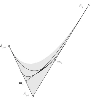
Let a non-rational cubic B-spline curves(u)with control pointsd_i,(i= 0, ..., n)and knot values u_k,(k= 0, ..., n+ 4) be given. Until now the only possibility for the modification of this curve has been the repositioning of its control points. Now we give an algorithm for changing this curve by modifying its knot values in such a way that the curve will pass through a given pointp at the given parameter valueu. This point, of course cannot be anywhere: the algorithm workse if this point is inside the region defined by the sides of the control polygon and the envelopes mentioned in Theorem 1.7, which are parabolic arcs in the cubic case.

Let point p be in the region defined by the control points d_j−2,d_j−1,d_j. Let a parameter value ue ∈ [u_j, u_j+2) be also given. Consider a quadratic B-spline curve b(v) with the same