https://doi.org/10.1007/s10479-020-03678-6 O R I G I N A L R E S E A R C H
Spectral risk measure of holding stocks in the long run
Zsolt Bihary1·Péter Csóka1,2 ·Dávid Zoltán Szabó3
Published online: 18 June 2020
© The Author(s) 2020
Abstract
We investigate how the spectral risk measure associated with holding stocks rather than a risk- free deposit, depends on the holding period. Previous papers have shown that within a limited class of spectral risk measures, and when the stock price follows specific processes, spectral risk becomes negative at long periods. We generalize this result for arbitrary exponential Lévy processes. We also prove the same behavior for all spectral risk measures (including the important special case of Expected Shortfall) when the stock price grows realistically fast and when it follows a geometric Brownian motion or a finite moment log stable process.
This result would suggest that holding stocks for long periods has a vanishing downside risk.
However, using realistic models, we find numerically that spectral risk initially increases for a significant amount of time and reaches zero level only after several decades. Therefore, we conclude that holding stocks has spectral risk for all practically relevant periods.
Keywords Coherent risk measures·Downside risk·Lévy processes·Finite moment log stable model·Time diversification
JEL Classification G11
We would like to thank Peter Farkas, Gabor Kondor, Adam Zawadowski, and participants of the 8th Annual Financial Market Liquidity Conference for helpful comments. Péter Csóka was supported by the
ÚNKP-17-4-III New National Excellence Program of the Ministry of Human Capacities and also thanks funding from National Research, Development and Innovation Office— NKFIH, K-120035.
B
Péter Csókapeter.csoka@uni-corvinus.hu Zsolt Bihary
zsolt.bihary2@uni-corvinus.hu Dávid Zoltán Szabó
szdavid89@gmail.com
1 Department of Finance, Corvinus University of Budapest, Budapest, Hungary
2 “Momentum” Game Theory Research Group, Centre for Economic and Regional Studies, Budapest, Hungary
3 Independent Researcher, Budapest, Hungary
1 Introduction
There has been tremendous interest both from practitioners and researchers on the question of how risky it is to hold stocks rather than a risk-free deposit in the long run. The existence of time diversification, meaning that the risk of holding stocks decreases with the time horizon, has profound effects on all long-term investments such as pension savings and target date funds. Industry practitioners hold the common wisdom that the longer the intended holding period for a portfolio, the more it should contain risky, rather than risk-free investments.
The academic literature on the topic is more controversial (Bennyhoff2009). Siegel (1998) showed that for investment horizons of at least 15 years, the risk of holding stocks (measured by realized variance) is lower than the risk of holding bonds or Treasury bills, and the risk of holding stocks is decreasing over time. However, Pástor and Stambaugh (2012) argue that stocks are more volatile in the long run from the perspective of an investor. The reason is that investors do not know the parameters of the stock price process (especially not the conditional expected return), and by making noisy predictions, at a 50-year horizon they face about 1.3 times higher return variance per year than at a 1-year horizon. Modeling the investors’ beliefs, Avramov et al. (2017) find that there could be investors who perceive that the mean reversion of stocks is weaker, and hence they consider stocks riskier in the long run.
One can consider the probability that at timetthe stock investment valueS(t)is smaller than the risk free deposit valueS0er t, whereS0is the initial investment andris a constant risk- free rate. This probability decreases witht, supporting the notion that the risk of the stock investment decreases with the holding period. However, as noted by Harlow (1991), this concept does not take into account the difference betweenS0er tandS(t), and this difference can, of course, be larger and larger astincreases.
Bodie (1995) approached the concept of risk differently by quantifying risk as the price of a put option that guarantees the risk-free payoutS0er tat timet. The price of the corresponding put option was found to be increasing ast increases, which can be interpreted as the risk of holding stocks increases over time. Wilkie (2001) criticized the methodology of Bodie (1995) by saying that if we wish to guarantee that we get at least the proceeds of a risk-free investment, then (since buying the option also has some costs) we have to invest everything in the risk-free investment, and pricing the option makes no sense. Moreover, Ferguson and Dean (1996) argued that the method of Bodie (1995) forces one to conclude that the risk of an asset relative to the risk of any other asset increases with the investment horizon, leading to a paradox.
Following Treussard (2006); Nguyen et al. (2012), we consider the risk of holding a stock rather than a risk-free deposit over time. More precisely, we analyze the spectral risk measure (Acerbi2002) of the loss variableY(t)= S0er t −S(t). IfY(t)is positive (negative), then the stock performs poorly (well), in comparison with the risk free money market account.
Spectral risk measures are coherent (Artzner et al.1999, 2007) and can be expressed as a weighted average of losses, with increasing weights for higher losses. Thus we can think of the spectral risk ofY(t)as a weighted average regret value associated with having bought the stock, rather than investing in a money market account.
As a special spectral risk, we consider Expected Shortfall (ES) (Acerbi and Tasche2002;
Rockafellar and Uryasev2002), which can be computed and estimated efficiently (Acerbi and Tasche2002) and is backtestable (Acerbi and Szekely2014). Moreover, in 2013 the Basel Committee of Banking Supervision took the decision (Basel Committee2013) of using ES
for capital adequacy internal models, underscoring the importance of ES as a practical risk measure.
To describe the possible evolution of stock prices, we consider different stochastic pro- cesses. Besides the standard geometric Brownian motion (GBM) model, we analyze the exponential Lévy model (see for instance Mandelbrot (1963), Bertoin (1996), McCulloch (1996), Cai and Kou (2011), Fu and Yang (2012), Egami and Oryu (2015), and Fusai and Kyriakou (2016)). The exponential Lévy process, of which GBM is a special case, offers more flexibility to model the jumps and the heavy tail behavior of stock prices. As an illustra- tion, we will investigate a particular exponential Lévy subclass called the Finite Moment Log Stable (FMLS) model (Carr and Wu2003). In the FMLS model, moments of the logarithmic return exist on the gain side, but are infinite on the loss side. However, all moments exist for the price process, as the name FMLS indicates. Thus the FMLS price process can capture heavier tails for losses, while free from complications due to infinite moments.
There are two distinct regimes where the long-time behavior of risk is different. Depending on the parameters of the stock price process (the driftμand the convexity adjustmentκ), we distinguish between a high growth regime (μ > r+κ) and a medium growth regime (r +κ ≥ μ > r). Our results extend those of Nguyen et al. (2012), since we treat the exponential Lévy model in general and the FMLS model in particular, and we have results for Expected Shortfall both in the GBM and in the FMLS models. We prove in case of a GBM stock process that in the high growth regime all spectral risk measures (including Expected Shortfall) will be negative at hight. We also investigate general exponential Lévy models and provide conditions under which in both at the high growth and at the medium growth regimes spectral risk will be negative at hight. For the FMLS model, we obtain the same results as for the GBM model, that is, in the high growth regime all spectral risk measures will be negative at hight.
This result would suggest that holding stocks for long periods has a vanishing downside risk. However, using realistic price process models, we find numerically that the spectral risk initially increases for a significant amount of time and reaches zero level only after several decades. This result indicates that holding stocks has spectral risk for all practically relevant periods. This conclusion is found to be insensitive to reasonable changes in parameters.
The structure of the paper is as follows. Spectral risk measures and their Choquet repre- sentation are given in Sect.2. Section3contains the investigated stochastic processes, Sect.4 provides the analytical results. Section5contains numerical results, Sect.6concludes.
2 Spectral risk measures
Consider the random variable X that represents the loss distribution of a portfolio at the future timet, as seen at the current time. Thus positive values ofXare representing losses, negative values ofXare representing profits. The set of the random loss variables is denoted byX.
Definition 2.1 The risk measureρ:X →Ris called acoherent risk measure(Artzner et al.
1999) if it satisfies the following properties:
• monotonicity:Y ≤X⇒ρ(Y)≤ρ(X),
• positive homogeneity:h>0⇒ρ(h X)=hρ(X),
• sub-additivity:ρ(X+Y)≤ρ(X)+ρ(Y),
• translation invariance:a∈R⇒ρ(X+a)=ρ(X)+e−r ta, wheree−r tis the discount factor at timet.
Throughout this paper we will assume a constant risk-free rater. The discount factore−r t is omitted in some papers, but it is especially important for us here, as we will investigate long horizons.
Coherent risk measures have a sound axiomatic foundation (Artzner et al.1999), can be related to Bellman’s principle, are supported by general equilibrium theory (Csóka et al.2007) and they can also capture liquidity risk (Acerbi and Scandolo2008). Moreover, coherent risk measures have also been used as an objective function in inventory problems (Ahmed et al.
2007; Philpott and De Matos2012) considered the incorporation of a time-consistent coherent risk measure into a multi-stage stochastic programming model.
As a prominent coherent risk measure, Expected Shortfall (ES) (Acerbi and Tasche2002;
Rockafellar and Uryasev2002) can be computed and estimated efficiently (Acerbi and Tasche 2002), and it is backtestable (Acerbi and Szekely2014). Moreover, in 2013 the Basel Com- mittee of Banking Supervision took the decision (Basel Committee2013) of using ES for capital adequacy internal models. Given a random loss variableX ∈X and a confidence levelα ∈ [0,1], ESα(X)is the average of the loss in the worst 100(1−α)% cases. As an example,α=90%, and ES90%is the average of the loss in the worst 10% of the cases.
To define ES formally in our setting, we need some more notation. Given a random loss variable X ∈X, letFX(x)= P[X ≤x]denote its distribution function. The generalized inverse of the loss distributionXis defined asFX−1(p)=inf{x|FX(x)≥p}.
Definition 2.2 Given a random loss variable X ∈X, forα ∈ [0,1), theExpected Shortfall of X atα, ESα(X)is defined as
ESα(X)=e−r t 1 1−α
1
α FX−1(p)dp. Forα=1, ES1, that is the (discounted) maximum loss, is defined as
ESα(X)=e−r tess. sup{X},
where ess. sup{X}represents the essential supremum of the random loss variableX.
Spectral risk measures (Acerbi2002) are also coherent and they are generalizing ES to get the weighted average of the losses with increasing weights as follows.
Definition 2.3 Given a random loss variableX ∈X, thespectral risk measure of X,ρφ(X) is defined as
ρφ(X)=e−r t 1
0
FX−1(p)φ(p)dp, whereφ∈L1([0,1]), and the following properties are true:
• φis positive;
• φis monotonically increasing;
• 1
0 |φ(p)|d p=1.
Note again that all the usual formulas are written for losses, not gains, and they are adjusted with thee−r tdiscount factor. As it is clear from its definition, ES is a spectral risk measure that we will use as a specific example in our numerical calculations. Interestingly, Miller and Ruszczy´nski (2008) considered a portfolio optimization problem with different risk measures including spectral risk measures.
We will work with spectral risk measures throughout this paper, but we will use an equiva- lent definition derived as a special case of Choquet integrals (Choquet1954). This formulation
also appears in decision theory to model uncertainty (see for instance Grabisch and Labreuche (2010) and Labreuche and Grabisch (2018)). Choquet integral risk measures (see for instance Sriboonchita et al. (2009)) are defined as follows.
Definition 2.4 Given a random loss variable X ∈X, theChoquet integral risk measure of X,ρh(X)is given by
ρh(X)=e−r t ∞
0
h(1−FX(x))dx+e−r t 0
−∞[h(1−FX(x))−1]dx,
whereh, the so-called distortion function (Wang1996) is non-decreasing and satisfiesh(0)= 0 andh(1)=1.
Nguyen et al. (2012) notes that for concave distortion functionshthere exists a connection between Choquet integral risk measures and spectral risk measures such that ifh(1−p)= φ(p), then ρh(X) = ρφ(X) for all X ∈ X. In this work, we will refer to spectral risk measures and Choquet integral risk measures interchangeably. A distortion functionh is non-degenerate, if there existsp>0 such thath(p) >0, or, equivalently, there existsq<1 such thatφ(q) >0.
Following Treussard (2006); Nguyen et al. (2012), we considerY(t)= S0er t −S(t)as the loss variable whose spectral risk we want to calculate using Definition2.4. IfY(t)is positive (negative), then the stock performs poorly (well), in comparison with the risk-free deposit. We can also think ofY(t)as a regret value associated with having bought the stock, rather than holding our investment in a risk-free deposit.
Throughout the paper, we will restrict our attention to non-degenerate distortion func- tions. This means that we preclude the degenerate maximum loss risk measure from further investigation.
3 Investigated models
Let{S(t)}t≥0 be a positive valued stochastic process which represents the stock price on the market. As usual, this stochastic process is assumed to be defined on a complete filtered probability space(,F,{Ft}t≥0,P).
In thegeometric Brownian motion model (GBM), the stock price follows the stochastic process
S(t)=S0e(μ−σ2/2)t+σWt, S(0)=S0, (1) whereμ >0 is the drift,σ >0 is the volatility, and{Wt}t≥0is a Wiener process.
The standardized log return of this process{S(t)}t≥0is distributed as ln(S(t)S0 )−(μ−σ2/2)t
σ√
t ∼[z], (2)
where[z]is the standard normal distribution function.
Exponential Lévyprocesses, of which GBM is a special example, offer more flexibility to model heavier tail behaviour. In the exponential Lévy model, the stock price follows the stochastic process
S(t)=S0e(μ−κX)t+Xt, S(0)=S0, (3)
whereXt is a Lévy process fully determined by its Lévy tripletT,μis the drift, andκXis the convexity adjustment term that can be calculated as
κX = 1
tlnEeXt. (4)
The convexity adjustmentκX plays the role of an exponential compensator in the sense that the process{e−κXt+Xt}t≥0is an({Ft}t≥0,P)-exponential-martingale. Note thatκXdoes not depend on time. We will denote the distribution function of the Lévy process at a given timetbyFt.
We will consider a specific exponential Lévy model, calledFinite Moment Log Stable (FMLS)model. In the FMLS model, the stock price movement follows the stochastic process (Carr and Wu2003)
S(t)=S0e(μ−κ)t+σLαt, S(0)=S0, (5) whereμis the drift,σ is the scale of volatility,Lαt is alpha stable distributed with shape parametersα ∈(1,2)andβ = −1, with scale parametertα1, and with zero mean, that is Lαt ∼S(α,−1,tα1,0)(see more details in Carr and Wu (2003)). Note that the only remaining free parameter for the distribution isα. Theα →2 limit corresponds to the GBM model.
Decreasingαresults in heavier tails for the losses. As before,κis the convexity adjustment term for the FMLS model, given as
κ= −σαsec(πα/2). (6)
Note thatκis positive due to the properties of thesecfunction, asα∈(1,2). Now the log return of theS(t)process becomes
ln S(t)
S0
=(μ−κ)t+σLαt, (7) therefore its distribution isS(α,−1, σt1α, (μ−κ)t)for a fixedt. Stable distributions have the following important property (see for example page 24 of Janicki and Weron (1994)).
Proposition 3.1 If X is an alpha stable distributed random variable X∼S(α, β,1,0)then γX+δ∼S(α, β, γ, δ)forδ >0andγ ∈R.
Using Proposition3.1we obtain
ln(S(t)S0 )−(μ−κ)t
σt1α ∼S(α,−1,1,0). (8)
We denote the distribution and density functions ofS(α,−1,1,0)atzbyα(z)andα(z), respectively.
4 Analytical results
The main question of this paper is the long horizon behavior of the risk curveρh(Y(t)). To give some insights, let us discuss some general qualitative features of the risk curve. Att=0, ρh(Y(0))=0, since initially the stock price is deterministic. Roughly speaking, there are two quantities affecting spectral risk, the mean and dispersion of the stock price distribution.
Greater mean leads to lower risk, while greater dispersion results in higher risk. For short times, the dispersion grows much faster than the mean, leading to initially increasing risk
curves. The question is whether risk starts to decrease at a certain time or keeps rising. If ρh(Y(t))becomes negative for a larget, it must have decreased from its positive maximum.
The above described qualitative features of the risk curve will be demonstrated with numerical examples in Sect.5.
As discussed in the literature (see Hull (2012) and Ross (2015)), we will work under the statistical (real-world) measure in this paper. There are two distinct regimes where the long-time behavior of risk is different. The case whenμ >r+κwe call thehigh growth regime. Whenr+κ ≥μ >r, we are in themedium growth regime. The caseμ≤r(low growth regime) is not realistic, as it would mean that the risky asset grows slower on average than the risk-free asset.
Nguyen et al. (2012) investigated two exponential Lévy Processes, GBM and exponential Poisson. They proved thath>c >0 is a sufficient condition in both regimes for the risk to be negative at hight. In the high growth regime, they also proved this behavior ifhis continuous. We reinvestigated the GBM model and proved the new result that in the high growth regime all spectral risk measures would be negative at hight. Moreover, for general exponential Lévy models, we proved that in both high growth and medium growth regimes ifh>c >0, then spectral risk will be negative at hight. We also investigated a specific exponential Lévy model, the FMLS model, and we obtained the same results as for the GBM model, that is in the high growth regime all spectral risk measures will be negative at hight.
4.1 GBM model
In this section, we assume that the stock processS(t)is a geometric Brownian motion.
The formula derived by Nguyen et al. (2012) for the spectral risk, adjusted to our definition that takes into account discounting, is:
ρh(Y(t))=S0[1−e(μ−r)t ∞
−∞h([z]) 1
√2πe−12(z−σ
√t)2dz]. (9)
We have the following own result.
Theorem 4.1 In the GBM stock price model,ρh(Y(t))is negative for a large t ifμ >r+σ22. Proof Sincehis a monotonically decreasing function in a closed interval, it can only have a countable number of jump points, so the function is almost surely continuous everywhere.
LetA= [0,d]. Since we only consider non-degenerate distortion functions,
h(x)≥c ∀ x ∈A, (10)
wherec>0. For the integral in (9), we obtain the following lower bound.
∞
−∞h([z]) 1
√2πe−12(z−σ
√t)2dz (11)
=
−1A
h([z]) 1
√2πe−12 (z−σ
√t)2dz+
R\−1A
h([z]) 1
√2πe−12(z−σ
√t)2dz
≥c
−1A
√1
2πe−12 (z−σ√t)2dz+
R\−1A
h([z]) 1
√2πe−12 (z−σ√t)2dz.
By definition,−1(A)= (−∞,b], whereb= −1(d). For every pointx on the interval (−∞,b]we haveh([x])≥c. Let us choose a subinterval[a,b]of the interval(−∞,b].
Sinceh≥0 everywhere, we can assess that ∞
−∞h([z]) 1
√2πe−12(z−σ√t)2dz (12)
≥c b
a
√1
2πe−12 (z−σ√t)2dz=c[(b−σ√
t)−(a−σ√ t)],
where the last equation follows from integrating the density function of a normally distributed random variable with meanσ√
tand standard deviation 1 on the interval[a,b]. Using the mean value theorem, for ad∈ [a,b]we assess that
c[(b−σ√
t)−(a−σ√
t)] ≥c(b−a)e−12 (d−σ√t)2.
Therefore, we can deduce that e(μ−r)t
∞
−∞h([z]) 1
√2πe−12(z−σ
√t)2dz (13)
≥e(μ−r)tc·(b−a)e−12(d−σ√t)2 =c·(b−a)e(μ−r−σ
2 2 )t+dσ√
t−12d2.
The last expression goes to infinity iftgoes to infinity, since we assumed thatμ−r−σ22 >0.
It follows thatρh(Y(t))in (9) goes to minus infinity and hence becomes negative for a large
t.
4.2 Arbitrary exponential Lévy models
In this section, we assume that the stock processS(t)is an exponential Lévy process. For a brief introduction, see Sect.3. First, we derive an own formula for the spectral risk in this model.
Theorem 4.2 In an arbitrary exponential Lévy model, the spectral risk of Y(t)is ρh(Y(t))=S0[1−e(μ−r)t
∞
−∞ez−κX(1)th(Ft(z))ft(z)dz], (14) where Ftis the distribution function of the Lévy process at a given time t, and ftis its density function.
Proof Using the Choquet representation in Definition2.4, we get that ρh(Y(t))=
∞
0
h(1−FY(t)(x))d x+ 0
−∞[h(1−FY(t)(x))−1]dx. (15) We conduct a substitution to express this formula with the distribution function of the Lévy process. To do so, we further shape 1−FY(t)(x). We know that the log return of the stock in this model can be written as
ln(S(t)
S0 )=μt+Xt−tκX. (16)
Using Eq. (16), we obtain the following
1−FY(t)(x)=P(S(t) <S0er t−x) (17)
=P
X(t) <ln
S0er t−x S0
−(μ−κX(1))t
=Ft
ln
S0er t−x S0
−(μ−κX(1))t . In Eq. (15), performing the substitution z = ln(er t − Sx
0) − (μ − κX)t ⇔ d x =
−S0ez+(μ−κX)td z, we get that ρh(Y(t))=
C
−∞h(Ft(z))S0ez+(μ−κX)tdz+ ∞
C
[h(Ft(z))−1]S0ez+(μ−κX)tdz, (18) whereC =(r−μ+κX)t. Integrating by parts, we obtain that
ρh(Y(t))= [h(Ft(z))S0ez+(μ−κX)t]C−∞− C
−∞h(Ft(z))ft(z)S0ez+(μ−κX)tdz (19) + [h(Ft(z)−1]S0ez+(μ−κX)t]∞C −
∞
C
h(Ft(z))ft(z)S0ez+(μ−κX)tdz.
Substituting the values on the boundary points usingh(0)=0,h(1)=1 we can assert that
ρh(Y(t))=S0er t[1−e(μ−r)t ∞
−∞ez−κXth(Ft(z))ft(z)dz].
Applying Theorem4.2, we prove the same long-time behavior for arbitrary Lévy models as was proven by Nguyen et al. (2012) in the case of GBM.
Theorem 4.3 In an arbitrary exponential Lévy modelρh(Y(t))is negative for a large t if h(·)is bounded below with a c>0constant, and ifμ >r .
Proof Due to the definition ofκXand by the assumption of the theorem ∞
−∞ez−κXth(Ft(z))ft(z)dz (20)
≥C· ∞
−∞ez−κXtft(z)dz=C·e−κXtE[eXt] =C. and therefore,
e(μ−r)t ∞
−∞ez−κX(1)th(Ft(z))ft(z)dz (21) goes to infinity astgoes to infinity, implying thatρh(Y(t))also goes to minus infinity and
ρh(Y(t))becomes negative for a larget.
4.3 FMLS model
In this section, we assume that the stock process S(t) is an FMLS process. For a brief introduction, see Sect.3.
Theorem 4.4 In the FMLS stock price model, the spectral risk of Y(t)is ρh(Y(t))=S0[1−e(μ−r)t
∞
−∞ezσt1/α−κth(α(z))α(z)dz]. (22) Proof The proof is similar to that of Theorem4.2. The main difference appears in the variable substitution. Due to the properties of the stable variables (Proposition3.1) we can express the risk without time dependency.
Performing the substitutionz = ln(er t−Sx0)−(μ−κ)t
σt1α ⇔d x = −S0σtα1ezσt
1α+(μ−κ)td z, integrating by parts and utilisingh(0)=0 andh(1)=1, we obtainρh(Y(t))as stated in the
theorem.
Theorem 4.5 In the FMLS stock price model,ρh(Y(t))is negative for a large t if h(·)is bounded below with a c>0constant, and ifμ >r .
Proof This is a special case of Theorem4.3, since the FMLS process is an exponential Lévy process.
Theorem 4.6 In the FMLS stock price model,ρh(Y(t))is negative for a large t ifμ >r+κ.
Proof Sincehis a monotonically decreasing function in a closed interval, it can only have a countable number of jump points, so the function is almost surely continuous everywhere.
LetA= [0,d]. Since we only consider non-degenerate distortion functions, h(x)≥c ∀ x ∈A,
wherec>0. As for the integral in (22), we obtain the following lower bound.
∞
−∞ezσt1/α−κth(α(z))α(z)dz (23)
=
−1α (A)ezσt1/α−κth(α(z))α(z)dz+
R\−1α (A)ezσt1/α−κth(α(z))α(z)dz
≥c
−1α (A)ezσt1/α−κtα(z)dz+
R\−1α (A)ezσt1/α−κth(α(z))α(z)dz.
By definition,−1α (A)= (−∞,b], whereb =−1α (a). For every pointx on the interval (−∞,b], it holds thath(α(x))≥c.
Next, we will show thatα(z)is positive on an appropriate subinterval[a,b]of[−∞,b]. We know thatα(z)is the density function of a stable distributed random variable with parameters(α,−1,1,0). Moreover, on[−∞,b]the cumulative distribution function of this random variable is not constant, hence the density function is surely positive at some points.
According to Proposition 3.12 on page 102 of Cont and Tankov (2004), if a Lévy process is infinitely active, then the density function of this process is continuous for everyt. Carr and Wu (2003) showed that the stable process is infinitely active in case 1< α < 2, meaning that it has an infinite number of jumps over any time interval. Hence we can assess that the processLα,−t 1 has continuous density function for everyt ≥ 0. In particular, it holds for t =1, that is forα(z). Thusα(z)is positive in at least one point on[−∞,b], implying thatα(z)is positive on an appropriate subinterval[a,b]of[−∞,b].
Denote the minimum value ofα(z)on[a,b]byc>0. Sinceh≥0 everywhere, we obtain that
e(μ−r)t ∞
−∞ezσt1/α−κth(α(z))α(z)dz (24)
≥c·e(μ−r)t b
a
ezσt1/α−κtα(z)dz= b
a
c·e(μ−r−κ)t+zσt1/αα(z)dz.
Sinceα(z)is positive on an appropriate subinterval[a,b]of[−∞,b], we obtain that e(μ−r)t
∞
−∞ezσt1/α−κth(α(z))α(z)dz (25)
≥c·c b
a
e(μ−r−κ)t+zσt1/αdz. By integrating, it follows that
b a
e(μ−r−κ)t+zσt1/αdz=e(μ−r−κ)t+zσt1/α σt1/α
b
a (26)
= e(μ−r−κ)t
σt1/α [ebσt1/α−aσt1/α] =e(μ−r−κ)t
σt1/α [e(b−a)σt1/α].
The last expression goes to infinity iftgoes to infinity, since we assumed thatμ >r+κ. It follows thatρh(Y(t))in (22) goes to minus infinity and hence becomes negative for a large t.
5 Numerical results
To illustrate the implications of our theoretical calculations, in this section we present numer- ical results performed with realistic model parameters. We obtained the daily closing prices on the dividend-adjusted SP500 index to represent the risky “stock” in our model. The cash deposit rate was estimated using data on the annualized returns on 3-month US treasury bills. Both time series were taken from 1960 to 2016. Calibrating the historical data to the GBM model yielded the following estimation for the parameters:r =0.048,μ= 0.089, σG B M=0.155.
To illustrate the effect of stronger tails in the loss distribution, and to offer some robust- ness test, we also calibrated a set of FMLS models with four different α parameters:
α= 1.8,1.85,1.9,1.95. We used the samer =0.048,μ=0.089 values as for the GBM model. At eachα, we setσα such that the difference between the first and the third yearly return quartiles are matched with that of the GBM model. This procedure ensures consistency between the different models in terms of short-term volatility. All five of these models rep- resent realistic test cases for long-term investments in a well-diversified US equity portfolio.
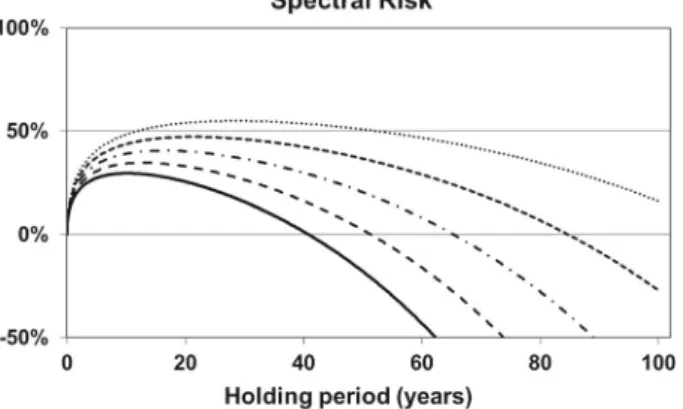
All the models are in the “high growth regime” as defined in Sect.4. Using our results from Sect.4, we computed the Expected Shortfall at the 90% level as an illustrative risk measure. We performed the calculation for all five calibrated models for different holding periods, up to one hundred years, with monthly steps. The value of the initial stock investment was set to unity. The distribution functions of the normal and stable distributions are readily available in MatLab, the necessary integrations were performed with numerical quadrature, also available in MatLab. The results are plotted in Fig.1. The risk curves start at zero,
increase up to a maximum value, then, in accordance with our analytical results, drop down to and below zero. At any given holding period, the GBM model produces the lowest risk levels, while the FMLS curves, especially the ones with relatively lowαparameters, show higher risk values. This is due to the heavier tails in the FMLS distribution on the loss side.
As discussed in the seminal paper of Artzner et al. (1999), coherent risk measures can be interpreted as the amount of reserve cash necessary to lower market exposure to a tolerable level. Although the numerical results shown underscore our analytic conclusion that the risk measure becomes zero at some holding time for all the investigated models, note the time scale on thexaxis. The necessary reserve cash becomes zero only at around, or beyond, one hundred years. The risk of holding stocks remains significant even after one hundred years, when the stock return distribution has heavy tails (see the curves with the smallest alpha values).
On the other hand, at long but realistic holding periods (a few decades), we need quite a sizable cushion to mitigate risk. According to Fig.1, the necessary cash reserve amounts to about half of the initial stock value.
Fig. 1 Expected Shortfall (90%) risk measure for holding a stock rather than a risk-free deposit, as a function of the holding period forr=0.048,μ=0.089, andσG B M=0.155. Risk curves are plotted for the GBM model, and for the FMLS model with differentαparameters
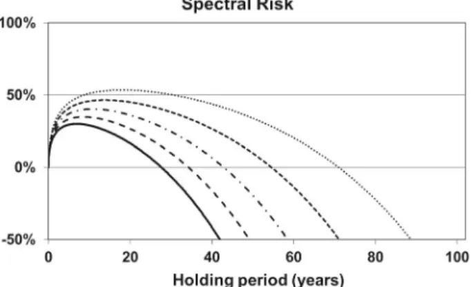
Fig. 2 Expected Shortfall (90%) risk measure for holding a stock rather than a risk-free deposit, as a function of the holding period forr=0.048,μ=0.089, andσG B M=0.125. Risk curves are plotted for the GBM model, and for the FMLS model with differentαparameters
Fig. 3 Expected Shortfall (90%) risk measure for holding a stock rather than a risk-free deposit, as a function of the holding period forr=0.048,μ=0.11, andσG B M =0.155. Risk curves are plotted for the GBM model, and for the FMLS model with differentαparameters
To perform some sensitivity tests, let us consider the effect of changing the parame- ters. In particular, we will explore parameter modifications that lower the risk measure. For most users, decreasing the 90% confidence level for the Expected Shortfall is not an option.
Increasing the confidence level would lead to higher risks, since then the average of even worse outcomes would be calculated. To decrease risk, volatility should be decreased or the difference betweenμandrshould be increased in our models. In Fig.2, we show risk curves with a reduced volatility ofσG B M = 0.125. In Fig.3, the curves are calculated with the increased drift ofμ=0.11. All other parameters are the same as in Fig.1. Our models with these modified parameters represent optimistic, but still realistic market views. Although the risk curves with the modified parameters shifted down as expected, our conclusions remain essentially the same: Risk remains significant for decades.
6 Conclusion
For long-run investors, it is crucial to know how to evaluate the risk associated with holding stocks rather than a risk-free deposit. We analyzed spectral risk, which can be interpreted as a weighted average regret value associated with having bought the stock, rather than investing in a money market account.
We show that for arbitrary exponential Lévy processes and when all possible outcomes have strictly positive weight, spectral risk becomes negative at long periods. We also prove the same behavior for all spectral risk measures (including the important special case of Expected Shortfall) when the stock price is in the high-growth regime and when it follows a GBM or an FMLS process.
We leave it as an open question whether Expected Shortfall becomes negative for arbitrary exponential Lévy processes in the high growth regime. Moreover, in a more realistic model, as well as in standard industry practice, for such long time horizons a stochastic interest rate model would be necessary. Since coherent measures of risk are extended to a dynamic setting with stochastic interest rates by Riedel (2004), it would be interesting to consider a model with a correlated joint distribution of the future stock price and the discount factor.
Our results show that in the long run, the steady growth of the expected stock price overrides its uncertainty in terms of the risk involved. However, how long is the long run in practice?
To answer this question, we calibrated the models to historical market data and performed numerical calculations. We find that the risk as defined in our paper indeed becomes negative, but it remains significantly positive for decades, even for optimistic market views. Increasing the tails in the FMLS process, or adding model or parameter uncertainty makes the situation even worse. Also supported by the sensitivity tests, our final conclusion is that holding stocks is risky for all relevant holding periods.
Acknowledgements Open access funding provided by Corvinus University of Budapest (BCE).
Open Access This article is licensed under a Creative Commons Attribution 4.0 International License, which permits use, sharing, adaptation, distribution and reproduction in any medium or format, as long as you give appropriate credit to the original author(s) and the source, provide a link to the Creative Commons licence, and indicate if changes were made. The images or other third party material in this article are included in the article’s Creative Commons licence, unless indicated otherwise in a credit line to the material. If material is not included in the article’s Creative Commons licence and your intended use is not permitted by statutory regulation or exceeds the permitted use, you will need to obtain permission directly from the copyright holder.
To view a copy of this licence, visithttp://creativecommons.org/licenses/by/4.0/.
References
Acerbi, C. (2002). Spectral measures of risk: A coherent representation of subjective risk aversion.Journal of Banking & Finance,26, 1505–1518.
Acerbi, C., & Scandolo, G. (2008). Liquidity risk theory and coherent measures of risk.Quantitative Finance, 8(7), 681–692.
Acerbi, C., & Szekely, B. (2014). Back-testing expected shortfall.Risk,27(11), 76–81.
Acerbi, C., & Tasche, D. (2002). Expected shortfall: A natural coherent alternative to value at risk.Economic Notes,31, 379–388.
Ahmed, S., Çakmak, U., & Shapiro, A. (2007). Coherent risk measures in inventory problems.European Journal of Operational Research,182(1), 226–238.
Artzner, P., Delbaen, F., Eber, J. M., & Heath, D. (1999). Coherent measures of risk.Mathematical Finance, 9, 203–228.
Artzner, P., Delbaen, F., Eber, J.-M., Heath, D., & Ku, H. (2007). Coherent multiperiod risk adjusted values and Bellman’s principle.Annals of Operations Research,152(1), 5–22.
Avramov, D., Cederburg, S., & Luˇcivjanská, K. (2017). Are stocks riskier over the long run? Taking cues from economic theory.The Review of Financial Studies,31(2), 556–594.
Basel Committee. (2013). Fundamental review of the trading book: A revised market risk framework. Con- sultative Document, October.
Bennyhoff, D. G. (2009). Time diversification and horizon-based asset allocations.The Journal of Investing, 18(1), 45–52.
Bertoin, J. (1996).Lévy processes. Cambridge: Cambridge University Press.
Bodie, Z. (1995). On the risk of stocks in the long run.Financial Analysts Journal,51, 18–22.
Cai, N., & Kou, S. G. (2011). Option pricing under a mixed-exponential jump diffusion model.Management Science,57(11), 2067–2081.
Carr, P., & Wu, L. (2003). The finite moment log stable process and option pricing.The Journal of Finance, 8(2), 753–778.
Choquet, G. (1954). Theory of capacities.Annales de l’institut Fourier,5, 131–295.
Cont, R., & Tankov, P. (2004).Financial modelling with jump processes. New York: Chapman and Hall/CRC.
Csóka, P., Herings, P. J.-J., & Kóczy, L. Á. (2007). Coherent measures of risk from a general equilibrium perspective.Journal of Banking & Finance,31(8), 2517–2534.
Egami, M., & Oryu, T. (2015). An excursion-theoretic approach to regulator’s bank reorganization problem.
Operations Research,63(3), 527–539.
Ferguson, R., & Dean, L. (1996). On the risk of stocks in the long run: A Comment.Financial Analysts Journal,52, 67–68.
Fu, J., & Yang, H. (2012). Equilibruim approach of asset pricing under Lévy process.European Journal of Operational Research,223(3), 701–708.
Fusai, G., & Kyriakou, I. (2016). General optimized lower and upper bounds for discrete and continuous arithmetic Asian options.Mathematics of Operations Research,41(2), 531–559.
Grabisch, M., & Labreuche, C. (2010). A decade of application of the Choquet and Sugeno integrals in multi-criteria decision aid.Annals of Operations Research,175(1), 247–286.
Harlow, W. V. (1991). Asset allocation in a downside-risk framework.Financial Analysts Journal,47(5), 28–40.
Hull, J. C. (2012).Risk management and financial institutions(Vol. 806). Hoboken: Wiley.
Janicki, A., & Weron, A. (1994).Simulation and Chaotic behavior of alpha-stable stochastic processes. New York: Marcel Dekker.
Labreuche, C., & Grabisch, M. (2018). Using multiple reference levels in multi-criteria decision aid: The generalized-additive independence model and the Choquet integral approaches.European Journal of Operational Research,267(2), 598–611.
Mandelbrot, B. (1963). New methods in statistical economics.Journal of Political Economy,71, 421–440.
McCulloch, J. H. (1996). Financial applications of stable distributions.Handbook of Statistics,14, 393–425.
Miller, N., & Ruszczy´nski, A. (2008). Risk-adjusted probability measures in portfolio optimization with coherent measures of risk.European Journal of Operational Research,191(1), 193–206.
Nguyen, H. T., Pham, U. H., & Tran, H. D. (2012). On some claims related to Choquet integral risk measures.
Annals of Operations Research,195, 5–31.
Pástor, L., & Stambaugh, R. F. (2012). Are stocks really less volatile in the long run?The Journal of Finance, 67(2), 431–478.
Philpott, A. B., & De Matos, V. L. (2012). Dynamic sampling algorithms for multi-stage stochastic programs with risk aversion.European Journal of Operational Research,218(2), 470–483.
Riedel, F. (2004). Dynamic coherent risk measures.Stochastic processes and their applications,112(2), 185–
200.
Rockafellar, R. T., & Uryasev, S. (2002). Conditional value-at-risk for general loss distributions.Journal of Banking & Finance,26(7), 1443–1471.
Ross, S. (2015). The recovery theorem.The Journal of Finance,70(2), 615–648.
Siegel, J. J. (1998).Stocks for the long run. New York: McGraw-Hill.
Sriboonchita, S., Wong, W.-K., Dhompongsa, S., & Nguyen, H. T. (2009).Stochastic dominance and appli- cations to finance, risk and economics. Boca Raton: CRC Press.
Treussard, J. (2006): The Non-Monotonicity of Value-at-Risk and the Validity of Risk Measures over Different Horizons.http://ssrn.com/abstract=776651.
Wang, S. (1996). Premium calculation by transforming the layer premium density.ASTIN Bulletin: The Journal of the IAA,26(1), 71–92.
Wilkie, D. (2001): On the Risk of Stocks in the Long Run: A response to Zvi Bodie. In: Proceedings of the 11th International AFIR Colloquium (pp. 741–762).
Publisher’s Note Springer Nature remains neutral with regard to jurisdictional claims in published maps and institutional affiliations.