10-07-15. TÁMOP – 4.1.2-08/2/A/KMR-2009-0006 1 Development of Complex Curricula for Molecular Bionics and Infobionics Programs within a consortial* framework**
Consortium leader
PETER PAZMANY CATHOLIC UNIVERSITY
Consortium members
SEMMELWEIS UNIVERSITY, DIALOG CAMPUS PUBLISHER
The Project has been realised with the support of the European Union and has been co-financed by the European Social Fund ***
**Molekuláris bionika és Infobionika Szakok tananyagának komplex fejlesztése konzorciumi keretben
***A projekt az Európai Unió támogatásával, az Európai Szociális Alap társfinanszírozásával valósul meg.
PETER PAZMANY CATHOLIC UNIVERSITY
SEMMELWEIS UNIVERSITY
10-07-15. TÁMOP – 4.1.2-08/2/A/KMR-2009-0006 1
2011.10.15. TÁMOP – 4.1.2-08/2/A/KMR-2009-0006 2
Peter Pazmany Catholic University Faculty of Information Technology
BEVEZETÉS A FUNKCIONÁLIS NEUROBIOLÓGIÁBA
INTRODUCTION TO
FUNCTIONAL NEUROBIOLOGY
www.itk.ppke.hu
By Imre Kalló
Contributed by: Tamás Freund, Zsolt Liposits, Zoltán Nusser, László Acsády, Szabolcs Káli, József Haller, Zsófia Maglóczky, Nórbert Hájos, Emilia Madarász, György Karmos, Miklós Palkovits, Anita Kamondi, Lóránd Erőss, Róbert
Gábriel, Kisvárdai Zoltán
2011.10.15. TÁMOP – 4.1.2-08/2/A/KMR-2009-0006 3
Introduction to functional neurobiology: Neuronal modelling
www.itk.ppke.hu
Neuronal modelling
Szabolcs Káli
Pázmány Péter Catholic University, Faculty of Information Technology
Infobionic and Neurobiological Plasticity Research Group, Hungarian Academy of Sciences – Pázmány Péter Catholic University – Semmelweis University
10-07-15. TÁMOP – 4.1.2-08/2/A/KMR-2009-0006 4
Neural modeling
Types of models:
•Descriptive – What is it like?
•Mechanistic – How does it function?
•Explanatory – Why is it like that?
10-07-15. TÁMOP – 4.1.2-08/2/A/KMR-2009-0006 5
How is information encoded by action potential trains?
Neurons respond to input typically by producing complex spike sequences that reflect both the intrinsic dynamics of the neuron and the temporal characteristics of the stimulus.
Simple way: Count the action potentials fired during stimulus, repeat the stimulus and average the results:
Some fundamental questions
Picture: Recordings from the visual cortex of a monkey. A bar of light was
moved through the receptive field of the cell at different angles (figure A). The highest firing rate was observed for input oriented at 0 degrees (figure B).
10-07-15. TÁMOP – 4.1.2-08/2/A/KMR-2009-0006 6
How to decode information encoded by action potential trains?
Example: Arm movement position decoding: If we take the average of the preferred directions of the neurons weighted by their firing rates, we get the arm movement direction vector.
Some fundamental questions
Picture: Comparison of arm position and arm position-sensitive neurons. The population activity was recorded in 8 directions. Arrows indicate vector sums of preferred directions, which is approximately the arm movement direction.
10-07-15. TÁMOP – 4.1.2-08/2/A/KMR-2009-0006 7
Why does a specific part of the brain use a specific type of
coding?
Example: Visual input noise filtering in ganglion cells: The structure of the receptive field changes according to the input signal-to noise ratio.Some fundamental questions
Solid curves are for low noise input (bright image), dashed lines are high noise input. Left: The amplitude of the predicted Fourier-transformed linear filters.
Right: The linear kernel as a function of the distance from the center of the receptive field
10-07-15. TÁMOP – 4.1.2-08/2/A/KMR-2009-0006 8
How do neurons as information processing units function; specifically, what is the relation between the temporal and spatial pattern of the input and the spatial and temporal pattern of the output?
Example:
Some fundamental questions
Picture: the effects of constant sustained dendritic current injection in a hippocampal pyramidal cell. The cell responds with a burst of spikes, then sustained spiking. In distal regions only a slow, large-amplitude initial response is visible, corresponding to a dendritic calcium spike.
10-07-15. TÁMOP – 4.1.2-08/2/A/KMR-2009-0006 9
How do neurons communicate, and what collective behaviors emerge in networks? Example: Orientation selectivity and contrast invariance in the primary visual cortex
Some fundamental questions
Left picture: schematics of a recurrent network with feedforward inputs.
Middle picture: The effect of contrast on orientation tuning. Figure A: orientation-tuned feedforward input curves for 80%,40%,20%,10% contrast ratios.
Right picture: The output firing rates for response to input in figure A.
Due to network amplification, the response of the network is much more
strongly tuned to orientation as a result of selective amplification by the recurrent network, and tuning width is insensitive to contrast.
10-07-15. TÁMOP – 4.1.2-08/2/A/KMR-2009-0006 10
How does cellular-level (synaptic) plasticity function? How can we understand behavioral-level learning? What is the connection
between the two? Example: The development of ocular stripes in the primary visual cortex
Left picture: schematics of the model network where right- and left- eye inputs from a single retinal location drive an array of cortical neurons.
Right picture: Ocular dominance maps, the light and dark areas along the cortical regions at the top and bottom indicate alternating right- and left-eye innervation. Top: In vitro measurements. Bottom: The pattern of innervation for the model after Hebbian development.
Some fundamental questions
10-07-15. TÁMOP – 4.1.2-08/2/A/KMR-2009-0006 11
Passive, isopotential (single compartment) neuron model
V : Membrane potential [V].
Ie : Current injected into the cell, with an electrode for example [A].
Q : Excess internal charge [C].
Rm : Membrane resistance, treated as a constant in the equations (specific membrane resistance, rm) [Ohm].
Cm : Membrane capacitance, treated as a constant in the equations (specific membrane capacitance, cm) [F].
The cell membrane is represented by a resistance and a battery in parallel with a capacitance.
10-07-15. TÁMOP – 4.1.2-08/2/A/KMR-2009-0006 12
Because of the principle of conservation of charge:
The time derivative of the charge dQ/dt is equal to the current passing into the cell, so the amount of current needed to change the membrane potential of a neuron with a total capacitance Cm at a rate dV/dt is CmdV/dt.
This is equal to:
Where Er is the resting potential of the cell. In most equations membrane conductance (gm) is used instead of resistance ( gm=1/rm ), because it is correlated with biophysical properties of the neuron:
Calculating the membrane current 1
10-07-15. TÁMOP – 4.1.2-08/2/A/KMR-2009-0006 13
The product of the membrane capacitance and the membrane resistance is a quantity in units of time, called the membrane time constant, denoted by tau:
The membrane time constant sets the basic time scale for changes in the membrane potential and typically falls in the range between 10 and 100 milliseconds.
Calculating the membrane current 2 : The membrane time constant
The total membrane conductance can change dynamically, causing the membrane time constant to change, too.
10-07-15. TÁMOP – 4.1.2-08/2/A/KMR-2009-0006 14
Response to current step at t=0
(ΔV = 100 mV, tau = 20msec, V0 = -70 mV)
The passive membrane behaves as a low-pass filter.
Example:
10-07-15. TÁMOP – 4.1.2-08/2/A/KMR-2009-0006 15
If there are multiple conductances (ion channels):
Equivalent electric circuit:
Where gi(V-Ei) is the current flowing through ion channel i.
Total current flowing through the membrane
Ion channels and synaptic channels can be represented as variable conductances.
Voltage-dependent conductances
Single ion channels are either in an open or a closed state. The probability of the states can depend on the membrane potential and on the binding of various substances (e.g. neurotransmitters) to the cell membrane.
10/15/2011 TÁMOP – 4.1.2-08/2/A/KMR-2009-0006 16
Figure: The currents passing through a single ion channel. In the open state, the channel passes -6.6pA at the holding potential of -140mV. This is equivalent to more than 107 charges per second passing through the channel.
10/15/2011 TÁMOP – 4.1.2-08/2/A/KMR-2009-0006 17
This means for the K+ ions to pass, 4 gates need to be open.
Example: In the case of the "delayed rectifier" K+ current:
Conductance per unit area of membrane for channel type i:
Where
Pi is the probability of a single channel being in the open state. This is approximately equal to the fraction of open channels (if the number of channels is large).
is the maximal conductance per unit area of membrane.
Structurally, ion channel pores have several gates, which all need to be open for current to flow through the channel.
The Hodgkin-Huxley model
Gating equation
10/15/2011 TÁMOP – 4.1.2-08/2/A/KMR-2009-0006 18
The transition of each gate is described by a kinetic scheme in which the gating transition closed-to-open occurs at voltage-dependent rate and the reverse transition occurs at rate
n is the probability that we find a gate open.
Left: example transition functions plotted as a function of the membrane potential
10/15/2011 TÁMOP – 4.1.2-08/2/A/KMR-2009-0006 19
Gating equation (other form)
The same equation in a useful form:
where
is called the time constant and
is the steady-state activation function.
Phenomenological models of synaptic conductances
• Exponential (for example AMPA type glutamate receptor)
• Difference of exponentials (for example GABAA). This method uses two time constants, thus both rise and decay can be described
• Alpha function
10/15/2011 TÁMOP – 4.1.2-08/2/A/KMR-2009-0006 20
This equation describes an isolated presynaptic release that occurs at t=0, reaches its maximum at the time constant, and decays with the time
constant.
Figure: Example alpha function with Pmax=200 and tau=30.
10/15/2011 TÁMOP – 4.1.2-08/2/A/KMR-2009-0006 21
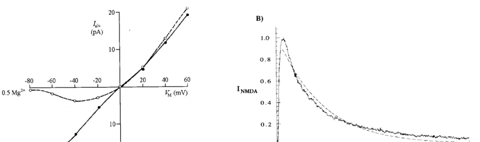
The NMDA-type glutamate synaptic receptor
Figure A: Current-voltage relations of the NMDA channel in the absence and in the presence of magnesium.
Figure B:
Jagged line: Experimentally recorded NMDA current.
Dotted line: computed NMDA current, with a double exponential time course.
The NMDA conductance depends not only on the binding of glutamate, but also on postsynaptic voltage (and the extracellular Mg2+ concentration).
The NMDA-type glutamate synaptic receptor
To describe the Mg2+ dependence of the NMDA channel an additional factor is introduced, which depends on the postsynaptic potential:
10/15/2011 TÁMOP – 4.1.2-08/2/A/KMR-2009-0006 22
Where P(t) is the open probability factor, and GNMDA(V) describes an extra voltage dependence due to the fact that near the resting potential NMDA receptors are blocked by Mg2+ ions, so to activate the conductance the postsynaptic neuron needs to be depolarized. This dependence can be approximated by a sigmoid function:
(typical fitted parameters: 1/η = 3.57 mM, 1/γ = 16.13 mV)
10/15/2011 TÁMOP – 4.1.2-08/2/A/KMR-2009-0006 23
The NMDA channel also conducts Ca2+ ions, which is important in plasticity.
The NMDA-type glutamate synaptic receptor
Figure: Dependence of the NMDA conductance on the membrane potential at different Mg2+ concentrations.
10-07-15. TÁMOP – 4.1.2-08/2/A/KMR-2009-0006 24
• Lots of different types of ion channels
• Complicated and cell-type dependent morphology
• The temporal and spatial pattern of synaptic input
• Neuromodulators, intracellular messenger molecules,...
Causes of more complex behavior in real neurons
Biophysically detailed multicompartmental models
Figure: The electrical circuit representation of three compartments in a multicompartmental model. Circles with V represent voltage-gated
conductances.
10-07-15.
Biophysically detailed multicompartmental models
The current flowing through compartment
where
is the total injected electrode current.
is the total surface area of the compartment.
are the resistive couplings to the neighboring compartments.
, with neighbors and
is the membrane potential of the compartment.
is the transmembrane current.
is the membrane capacitance of the compartment.
10-07-15. TÁMOP – 4.1.2-08/2/A/KMR-2009-0006 27
If the membrane potential reaches a threshold, the cell fires an action potential, and the membrane potential is set to a „reset potential”.
Simplest firing model: passive „integrate-and-fire”
Integrate-and-fire model
Or:
Picture: Membrane potential trace of an integrate-and-fire model (Ie is the injected current).
10-07-15. TÁMOP – 4.1.2-08/2/A/KMR-2009-0006 28
In the case of constant current injection, the analytic solution:
Integrate-and-fire model
Picture: integrate-and fire models compared to in vitro recordings.
Left: Firing rate as a function of the injected current. Continuous line:
model results; filled circles: Results for the first two spikes fired, in vivo recordings; open circles: steady-state firing frequency, in vivo recordings.
Middle: In vivo recording from pyramidal cell.
Right: voltage trace of the adaptive integrate-and-fire model.
The adaptation of the firing rate and refractory states are relatively easy to implement.
Firing-rate-based models
10/15/2011 TÁMOP – 4.1.2-08/2/A/KMR-2009-0006 29
Picture: Synaptic inputs to a single neuron.
u: Input rate vector. Denotes firing rate, not the membrane potential.
w: Synaptic (input) weight vector. For excitatory synapses w(i)>0, for inhibitory w(i)<0
v: Output rate vector. In the case of a single neuron, it has only one element.
10/15/2011 TÁMOP – 4.1.2-08/2/A/KMR-2009-0006 30
Ks(t) is the synaptic kernel function, which describes the time course of the synaptic current in response to a presynaptic spike arriving at time t=0.
Properties:
Synaptic kernel
Example:
If an action potential arrives at t=0 at input b, the synaptic current
generated at the postsynaptic neuron at time t is wbKs(t), where Ks(t) is the synaptic kernel.
10/15/2011 TÁMOP – 4.1.2-08/2/A/KMR-2009-0006 31
1. Calculating the total (somatically measured) synaptic current
where
is the neural response function, which describes the sequence of spikes fired by presynaptic
neuron b.
is the Dirac-delta function.
Nu is the number of input neurons.
tb,i is the time when a presynaptic spike occurs at input b.
The total synaptic current at time t:
10/15/2011 TÁMOP – 4.1.2-08/2/A/KMR-2009-0006 32
If the synaptic kernel is exponential:
Then differentiating (1) gives:
If the neuron response function is replaced by the firing rate of neuron b, denoted by
(1)
1. Calculating the total (somatically measured) synaptic current
2. Calculating the firing rate: activation function
To complete the firing rate model we must determine the postsynaptic firing rate v from Is.
For a constant input v=F(IS), where F is the activation function. It can be a sigmoid function, or - most frequently - linear function with a threshold:
10/15/2011 TÁMOP – 4.1.2-08/2/A/KMR-2009-0006 33
where
is the threshold (measured in Hz), and
is the half wave rectification operator: For any x
For convenience we assume that Is is multiplied by a constant which converts nA to Hz.
10/15/2011 TÁMOP – 4.1.2-08/2/A/KMR-2009-0006 34
Steady-state output fire rate
If all the inputs are time-independent (or in steady-state), the total current is:
Is=wu.
As a consequence the steady-state output firing rate is:
Where w is the synaptic weight vector and u is the synaptic input vector.
This equation describes how the neuron responds to constant (time- independent) current.
10/15/2011 TÁMOP – 4.1.2-08/2/A/KMR-2009-0006 35
If IS(t) is time-dependent:
and
In this case it is assumed that the firing rates follow the time-varying currents instantaneously.
Other model:
The time-dependent firing rate is modeled as a low-pass filtered version of the steady-state firing rate:
Firing-rate model with time-dependent dynamics
Where
is a time constant that determines how rapidly the firing rate approaches its steady-state value for constant Is.
10/15/2011 TÁMOP – 4.1.2-08/2/A/KMR-2009-0006 36
If
meaning that the firing rate time constant is much larger than the
synaptic rate time constant, then we can replace the time-dependent synaptic current function ( Is(t) ) with the total steady-state current (wu):
In other words, it is assumed that the firing rate is a low-pass filtered version of the input current.
Firing-rate model with time-dependent dynamics
Feedforward and recurrent networks
10/15/2011 TÁMOP – 4.1.2-08/2/A/KMR-2009-0006 37
Picture A: Feedforward network.
Picture B: Recurrent network with feedforward inputs.
W: Feedforward synaptic weight matrix, where Wab is the strength of the synapse from input unit b to output unit a.
M: Synaptic weight matrix for the recurrent layer.
Feedforward and recurrent networks
Output firing rates in feedforward networks (fig. A):
or
Adding the recurrent connections (fig. B):
10/15/2011 TÁMOP – 4.1.2-08/2/A/KMR-2009-0006 38
If we distinguish excitatory and inhibitory populations:
(h=Wu)
Another frequent abstraction:
(symmetric recurrent connections) —> simpler dynamics These two assumptions are seemingly contradictory, but can be reconciled if we assume that inhibition is much faster than excitation.
Then steady-state inhibitory activity can be substituted into the first equation, and the effective interaction between excitatory neurons can be symmetric with appropriate weight matrices.
10/15/2011 TÁMOP – 4.1.2-08/2/A/KMR-2009-0006 39
Coordinate transformation in feedforward networks
Reaching for a visible object requires a transformation from (retinal) sensory coordinates to body-centered motor coordinates.
10/15/2011 TÁMOP – 4.1.2-08/2/A/KMR-2009-0006 40
s is the location of the target in retinal coordinates.
g is the gaze angle, indicating the direction of gaze relative from the axis of the body.
s+g is the direction of the target relative to the body.
10/15/2011 TÁMOP – 4.1.2-08/2/A/KMR-2009-0006 41
In the premotor area of the frontal lobes
Neural coordinate transformations
Picture:
Firing rates of a visually responsive neuron in the premotor cortex of a monkey. Visual stimuli were incoming objects at various angles.
A: The response tuning curve does not change with eye position.
B: If the monkey’s head is turned 15 degrees to the right, the tuning curves shift by 15 degrees too.
C: Model turning curves at -20,0,10 degrees. (dotted, solid, heavy dotted)
Possible intermediate representation (in area 7a of the parietal lobe)
Question: Can we combine the activity of such neurons in a feedforward network to create output neurons firing in body-centered coordinates?
Can be modeled by the product of a Gaussian function of s and a sigmoid function of g; the activity of various neurons of the population is
is the center of the sigmoid.
is the mean of the Gaussian and where
10/15/2011 TÁMOP – 4.1.2-08/2/A/KMR-2009-0006 42
Linear recurrent networks
Multiplying by the eigenvector
Let us assume that M is symmetric —> real eigenvalues
and orthogonal eigenvectors forming a basis, so we may write
and substituting into (1),
10/15/2011 TÁMOP – 4.1.2-08/2/A/KMR-2009-0006 43
(1)
This transformation could also be implemented by a purely feedforward network!
For time-independent inputs the solution is:
If for any ν, the network is unstable.
If exponentially approaches the stationary value with the time constant
10/15/2011 TÁMOP – 4.1.2-08/2/A/KMR-2009-0006 44
Linear recurrent networks
The steady-state value for v(t) is:
Applications of linear recurrent networks
1. Selective amplification
Assume that is very close to 1, and all other eigenvalues are signif- icantly smaller. Then the steady state is
10/15/2011 TÁMOP – 4.1.2-08/2/A/KMR-2009-0006 45
The response of the network is dominated by the projection of the input vector along the axis defined by e1, in other words it encodes an amplified version of the input onto e1.
Strength of amplification:
Continuously parametrized neuronal populations
Picture: In primary visual cortex, a neuron may be characterized by the orientation of its preferred stimulus (θ). These neurons tend to fire at the highest frequencies if the stimulus is at a specified angle in their receptive field.
To model such networks, it is more efficient to index neurons by their (continuously varying) preferred parameters.
We can replace the discrete population with a continuous population:
firing rates, synaptic weights.
Then the equation describing the dynamics becomes:
10/27/2010 TÁMOP – 4.1.2-08/2/A/KMR-2009-0006 46
10-07-15. TÁMOP – 4.1.2-08/2/A/KMR-2009-0006 47
Applications of linear recurrent networks: Selective amplification
If the neurons are described by a preferred value of a periodic variable (θ), and M(θ,θ’)~cos(θ-θ’), the network selectively amplifies the first Fourier component of the input:
Picture A: The input as a function of the preferred angle
B: The activity of the network as a function of the preferred angle. Input stimulus was the same as in picture A.
C: The Fourier transform amplitudes of the input.
D: The Fourier transform amplitudes of the output.
10/15/2011 TÁMOP – 4.1.2-08/2/A/KMR-2009-0006 48
For
h=0, the network sustains its activity, which acts as a memory of the integral of previous inputs. In other words the network
"remembers" the previous state.
2. Input integration
(h=Wu)
Example: network for storing eye position, which integrates the output of brainstem ocular motor neurons
Picture: Integrator neuron activity that is involved in horizontal eye positioning.
Problem: the eigenvalue must be really close to 1
10/15/2011 TÁMOP – 4.1.2-08/2/A/KMR-2009-0006 49
2. Input integration
Nonlinear recurrent networks
In biological neural networks firing rates must be positive.
Taking this into account:
where
The previous continuous model now becomes
10/15/2011 TÁMOP – 4.1.2-08/2/A/KMR-2009-0006 50
is the half wave rectification operator.
Selective amplification in the nonlinear case:
10/15/2011 TÁMOP – 4.1.2-08/2/A/KMR-2009-0006 51
Picture: Selective amplification in a linear network with A: The noisy input as a function of the preferred angle
B: The steady-state output as a function of the preferred angle. Input stimulus was the same as in picture A.
C: The Fourier transform amplitudes of the input.
D: The Fourier transform amplitudes of the output.
10/15/2011 TÁMOP – 4.1.2-08/2/A/KMR-2009-0006 52
Orientation selectivity and contrast invariance in V1
Selective amplification in the nonlinear case: Recurrent model of simple cells in the primary visual cortex.
Picture: The effect of contrast on orientation tuning
A: The feedforward input as a function of preferred orientation. Contrast ratios are (from top to bottom): 80%, 40%, 20%, 10%
B: The output firing rates in response to the inputs in figure A.
C: Tuning curves measured experimentally.
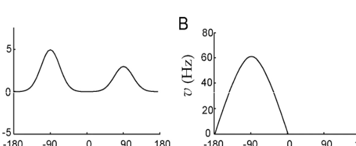
Input selection in nonlinear networks: Winner-takes-all input selection.
10/15/2011 TÁMOP – 4.1.2-08/2/A/KMR-2009-0006 53
Figure A: The input to the network consisting of two peaks.
Figure B: Network response. The output has a single peak at the location of the higher of the two peaks of the input.
10/15/2011 TÁMOP – 4.1.2-08/2/A/KMR-2009-0006 54
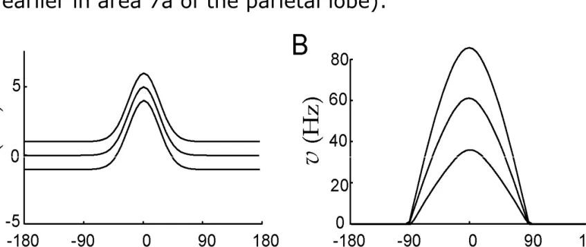
(as seen earlier in area 7a of the parietal lobe):
Input selection in nonlinear networks: Gain modulation
Picture: Effect of adding a constant to the input.
Figure A: The input to the network with one peak, with different amounts of added gain input.
Figure B: Network response. The higher gain yields a higher output.
Application: short-term (working) memory; the network "remembers"
the preceding stimulus even in the absence of external input.
10/15/2011 TÁMOP – 4.1.2-08/2/A/KMR-2009-0006 55
Input selection in nonlinear networks
Picture: response to varying input.
A,B: Input and output, with constant background and localized excitation.
C,D: After switching to a constant input, the response characteristics are the same
Maximum likelihood estimation
The above computations can also be interpreted as (nonlinear) regression, and may be used to approximate the "maximum likelihood" estimate of the value encoded by a noisy input.
The standard deviation of the estimate is
•4.5o for a simple "vector decoder"
•1.7o for recurrent network "cleanup" followed by vector decoding
•0.88o for the optimal (real maximum likelihood) decoder (Cramer-Rao lower bound)
10/15/2011 TÁMOP – 4.1.2-08/2/A/KMR-2009-0006 56
Associative (long-term) memory
As we have seen, recurrent networks often have activity patterns which behave as fixed point attractors. These may also be considered as stored memory traces, provided that we can specify the fixed points (preferably via a plausible activity-based learning rule).
Autoassociative function: the dynamics of the network reconstructs the original pattern based on a fragment or a noisy version.
10/15/2011 TÁMOP – 4.1.2-08/2/A/KMR-2009-0006 57