2 3 ENTROPY (f) FOR SIMPLE COOLING, \ FOR PRIOR EXPANSION, Τ FOR PRIOR COMPRESSION Fig. IB. Ideal Secondar

THE E F F E C T OF S E C O N D A R Y W A S T E H E A T O N S P A C E V E H I C L E R A D I A T O R A R E A

Calvin C. Silverstein

Cornell Aeronautical Laboratory, Inc. * Buffalo, Ν. Y .

Abstract

Equations are developed in dimensionless form for the specific radiator area (area per unit of generated power) of a space power plant when secondary waste heat is present in addition to waste heat from inefficient conversion of thermal power. Temperature ratios are obtained which minimize the

specific radiator area, and minimum areas corresponding to the optimum temperature ratios are calculated. The specific radiator area for an ideal fluid and the Carnot cycle, modified to allow for inefficient compression or expansion, is com­

pared with that for real fluids and the Rankine cycle. Oper­

ating conditions for which the idealized analysis is a good ap­

proximation to the performance of real fluids are determined.

Introduction

In any device which converts thermal energy to shaft work, a fraction of the thermal energy introduced to the device r e ­ mains unconverted, and hence must be removed to maintain temperature equilibrium. Such energy will be termed primary waste heat. If the energy conversion device is mounted in a spacecraft, radiation is the only feasible means for waste heat removal.

A significant fraction of generated power ultimately will be converted back to thermal form as the result of mechanical friction and electrical resistance. In a spacecraft, additional heat may result from the leakage of thermal energy from the energy conversion device prior to conversion, from metabolic processes in living things, and from absorption of thermal radiation emitted by other bodies in space.t Heat arising from

* P r e s ent Addr e s s : Atomics International, C a n o g a P a r k , Calif.

tThe effect on radiator area of thermal radiation from other bodies in space is generally small for radiator temperatures of interest, and will not be considered further ( I ) .

157

References 5 and 6 consider the problem in which a specified temperature level within a space vehicle is to be maintained by removal of secondary waste heat which leaks into the inte­

rior from a hot external skin, or is generated within the space­

craft cabin.

In this paper a general analysis of the problem of heat rejection from space power plants is presented, with the ob­

ject of determining the extent to which secondary waste heat influences radiator area.

Definition of P r o b l e m

It is assumed that the energy conversion device in a space­

craft power plant consists of a thermal energy source, a vapor turbine for the production of shaft power, a radiator-condenser for the rejection of p r i m a r y waste heat, and a liquid pump.

Both the Car not and Rankine power cycles, modified to allow for inefficient expansion, are used. Separate radiators are provided for the rejection of p r i m a r y and secondary waste heat.

Three methods for the removal of secondary waste heat are considered. In simple cooling, an appropriate coolant is circulated through components where secondary heat appears and then passes directly to the secondary radiator.

In the second method, the coolant temperature is raised by compression prior to entering the radiator. The increased coolant temperature in the radiator reduces the size of the radiator area needed to reject a unit of thermal power at the expense of shaft power used in the compression process. In the third method, the coolant temperature is lowered by ex­

pansion through a turbine prior to entering the radiator. While the radiator area needed to reject a unit of thermal power in­

creases in this case because of the lower coolant temperature, additional shaft power is produced. As will be shown, each cooling mode is optimum for a specified range of operating conditions.

F o r simple cooling, it is assumed that the coolant evapo­

rates at constant temperature, is condensed at constant tem­

perature in the radiator, and then is returned to the secondary heat source. Coolant pui.iping requirements are considered negligible.

158

When the coolant is compressed prior to entering the radiator, the various processes involved are represented by the reversed Carnot or Rankine cycles, modified to allow for inefficient compression. The reversed Rankine cycle is fur­

ther modified in that heat is rejected from the coolant only until the coolant becomes a saturated liquid. The coolant is then expanded via a throttling process to a temperature at which secondary waste heat can be absorbed.

When the coolant is expanded prior to entering the radi­

ator, the processes involved are identical to those occurring in the p r i m a r y power cycle.

The temperature of the coolant after removing secondary waste heat is assumed to be equal to the (constant) tempera­

ture of the secondary heat source. The temperature of the coolant while rejecting heat in the secondary radiator is as­

sumed to be equal to the (constant) radiator temperature.

The Carnot and r e v e r s e d Carnot cycles, with provision for inefficient expansion and compression, are called ideal cycles. The working fluid used is called an ideal fluid, and is characterized by zero specific heat while in the liquid state.

The Rankine and reversed Rankine cycles, with provision for inefficient expansion and compression, are termed real cycles and employ a real working fluid. As has been pointed out by Mackey Q.), as the specific heat of the real working fluid in liquid form approaches zero, the real fluid approaches the characteristics of the ideal fluid and the real cycles become identical to the ideal cycles.

The analysis is c a r r i e d out in terms of the specific radi­

ator area, defined as the total radiator area per unit of net generated power. Net generated power is defined as the dif­

ference between heat addition and rejection rates in the power cycle plus the difference between heat addition and rejection rates in the secondary coolant cycle. According to this defin­

ition, losses arising from friction and electrical resistance are not involved in the determination of net power, but instead are included in the secondary waste heat load. Also, second­

ary coolant power consumption or production is assumed to be taken directly off or added to the shaft of the power cycle turbine.

Ideal Cycle Analysis

Fig. 1A shows how the ideal power cycle appears on the temperature-entropy diagram. Saturated vapor at point a and temperature Tj expands through a turbine with efficiency 7 7 ^ , generating W units of power. After expansion the temperature of the working fluid has dropped to T^ at point b ' . Wet vapor then enters the primary radiator, where heat is rejected at

159

-r LU §2 ENTROPY (S) Fig. 1A. Ideal Power Cycle,

β

2 3

ι4ο

constant temperature until the working fluid becomes a satu­

rated liquid at point c. The saturated liquid is compressed to the subcooled state at c with negligible expenditure of energy.

The temperature of the subcooled liquid is increased to T\ at point d, where the saturated liquid state is reached. Energy is not required to change the temperature of the liquid, since its specific heat is postulated to be zero. Heat from the power plant energy source is then added at constant temperature to the working fluid, increasing its entropy until point a is reached and the cycle has been completed.

The possible secondary coolant cycles are illustrated in Fig. I B . Simple cooling followed by heat rejection in the sec­

ondary radiator is represented by the cycle: e-f-e. Cooling followed by expansion of the secondary coolant prior to enter­

ing the radiator is represented by the cycle: e - f - g ' - h - e . Cool­

ing followed by compression of the secondary coolant prior to entering the radiator is represented by the cycle: e - f - j ' - k - e . Between points h and k, the secondary coolant is assumed to be a subcooled liquid with zero specific heat; therefore, energy is not required to change the coolant temperature between these points. The expansion and compression efficiencies are denoted by 7 7S.

The specific radiator area can be expressed as: ( A + £a^)/

(W + 2^wi ) ? where A is the primary radiator area needed to i

reject power cycle waste heat, W is the power generated in the power cycle, a^ is the secondary radiator area needed to reject waste heat from the ith secondary waste heat source, and wi is the power consumption (negative) or power output (positive) of the i^ⁿ secondary coolant cycle.

The dimensionless specific radiator area φ is obtained by dividing the specific radiator area by the radiator area which would be needed to reject one unit of power at the maximum power cycle temperature. The latter area is just (€ σ T ^ ) ~ , where € is the radiator emissivity, C is the Stefan-Βoltzmann constant, and Tj is the maximum power cycle temperature.

Therefore,

Α +

Σ^

φ = ( 6 σ^Τ, ) 1 (1)

w +

Σ

i

When secondary waste heat is not present, the corresponding form for φ = φ0 is:

4\ A

141

Simple cooling:

P r i o r expansion:

Φ = Φ. = Φ + \

Φ

, δ =

7 7 3 ( 1

"

3

Μ ° 1 _{ι +}

— „ — „ , δ< ι

_- s)

P r i o r compression: φ (β*)

ι + ( 8 - ΐ)

(δ - ΐ) δ >

In the above equations, d is the ratio of the secondary waste heat production rate to power generated in the power cycle, β is the ratio of the temperature of the secondary waste heat source to the maximum power cycle temperature, ο is the ratio of the secondary radiator temperature to the temperature of the secondary waste heat source, *η ^s is the expansion or compression efficiency in the secondary coolant cycle, and Φο is the dimensionless specific radiator area when second­

ary waste heat is negligible ( α = 0). Note that as δ—*·1?

Eqs. (3) and (4) become equal to Eq. (2).

It can be shown that

1 - η (1 - r )

Φο= - - 4 <5)

V

-

where τ is the ratio of minimum power cycle temperature to maximum power cycle temperature and 77^. is the expansion efficiency in the power cycle.

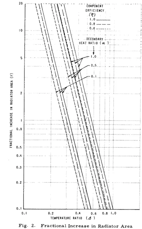
The fractional increase in radiator area F for simple cooling is:

Φ ι -

Φ.

Φο β⁴φ⁰

142

F is shown as a function of β in F i g . 2. The value of φ ^Q used in calculating F was φοπι> ^^{n e} minimum dimensionless specific a r e a when α = 0 (see Table 1). The large increase in radiator area as β decreases is evident.

If φ is divided by φ⁰ , the result is the ratio of radiator areas with and without secondary heat for the same net power output. The radiator a r e a ratio φΙφ⁰ will be called R, and is readily obtained f r o m E q s . (2), (3). and (4).

The value of τ for which R is minimized is found to be:

8η - 5 + 7 25 - I 6 77^t

m (7)

Both R and φ⁰ are minimized by the same value of τ . r ^m and corresponding values of φοχη, the minimum qb⁰, are given in Table 1 for several values of 7j^t.

Table 1. Optimum Values of r and φ

Vt Φοιη

1.0 0.750 9.50

0.8 0.765 12.63

0.6 0.775 17.80

The temperature ratio r ^m varies only slightly with Tjt, while the dimensionless specific radiator area φ^{ο τ η} increases substantially as rj^t is reduced.

Next, minimization of R with respect to the temperature ratio δ will be considered. The derivatives of E q s . (3) and (4) will be zero if the following relationships are satisfied:

0¹

ι

δ ⁴ ώ ι

"4(1 + a i 7^g) ( l

4 α η δ 's m

a( 5 - 877 ) + 3 8 m < 1 (8) m

a ( 8 - 5 i 7 ) + 377 - 4 αδ

4 's 's m

4 ( 7 7^s + o ) ( l - 77^g) m

, S ^m> l( 9 )

145

O . I 0 . 2 0 Λ 0 . 6 0 . 8 1 . 0 TEMPERATURE RATIO (so )

Fig. 2. Fractional Increase in Radiator A r e a for Simple Cooling.

where S^m is the value of δ for which R is a minimum.

A s Sm approaches unity in E q s . (8) and (9), β approaches the limits /3U and β^ , expressions for which are given below.

lirr^ ^

= 0 o

|

lim β \ = % \ = ⁴V " (1 + «> , S ^m > l (11) δ **

ι

m

In general. /3^U > β% . In the special case when 77 = 1,

£u = £ l .

When δ^{η ι} < 1, β > /3^U, as may be shown by comparing /3⁴ in Eq. (8) with β^u^ in Eq. (10). Determination of the relative magnitude of β when ô m — 1 is more involved. It can be shown that β < /3i when ô ^m > 1, and βι ^ β β^η when B^m = 1.

provided that 77 > 0.4. The situation when 77 < 0.4. of less practical interest, is modified from that described above.

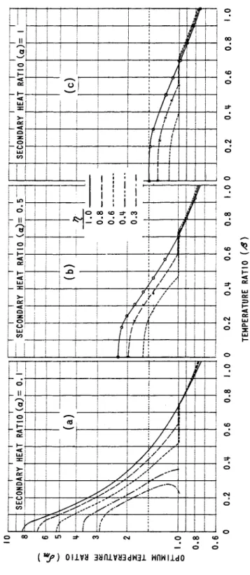
In Fig. 3, the optimum temperature ratio ô ^m is shown as a function of β, α, and 77. (It is assumed that 7 7t = r)s = T). ) F o r small values of β and a, the optimum secondary radiator temperature may be a factor of several greater than the tem­

perature of the secondary waste heat source. F r o m Fig. 3 one can obtain the range of β within which prior coolant compres­

sion, prior expansion, or simple cooling is the p r e f e r r e d mode of operation, as well as the optimum value of δ. For exam­

ple, observe the curve for α = 0.5 and 7 7 = 0.8. When β is less than 0 . 6 ( ^ ) , δ^{Γ Λ} is greater than one, indicating that the specific radiator area is minimized by prior compression of the coolant. Similarly, when β exceeds 0 . 7 2 ( βα) , ô m is less than one, and the specific radiator area is minimized by ex­

pansion of the coolant before entering the radiator. When β lies in the range 0.6 β ^ 0.72, equals one, and simple cooling yields minimum radiator area.

The unusual behavior of the ô ^m yj3 β curves which oc­

curs when 77 < 0.4 is shown in Fig. 3A only. The curve for 77 = 0.4 divides the family of curves for which a single value of &m exists (to the right) from the family for which two val­

ues of ô ^m exist over a limited range of /5(to the left). For the curve for which 77 = 0.3, two values of δηι exist over the range 0.226 < β < 0.276.

The values of ô m obtained from Fig. 3, along with φο τ η

from Table 1, can be substituted in E q s . (2), (3), and (4) to

145

Fig. 3. Optimum Ratio of Secondary Radiator Temperature to Secondary Waste Heat Source Temperature.

obtain the minimum dimensionless specific radiator area

<ji>

.

Division of φτη by

Φοτη

ondary waste heat becomes a significant and eventually a dom­

inant factor in determining the specific radiator area.

Although the minimum radiator area is of principal im­

portance in design calculations, it is also of interest to note how the minimum area compares with the radiator area when the simple cooling mode is used for the removal of secondary waste heat. If the difference is not great, the additional equip­

ment required for compressing or expanding the coolant to minimize the radiator area may not be warranted. In Fig. 5,

φχη/φΐ, the ratio of the minimum radiator area to that r e ­ quired for simple cooling, is shown as a function of β for various values of α and 77.

It can be seen that if β exceeds 0.52, the area ratio is larger than 0.90. That is, the minimum radiator area is at most only 10% less than that for simple cooling. This improv- ment would not seem to be warranted unless area restrictions are extremely critical. Therefore, simple cooling appears to be the preferred mode of secondary waste heat removal when

β}L 0.5. The fractional increase in radiator area for this case is readily obtained from F i g . 2 or Eq. (6). When β < 0.5,either prior compression or simple cooling should be employed, the choice being aided by examination of Fig. 5.

F r o m Fig. 5, it is evident that optimization of the temper­

ature ratio 8 is generally most effective in reducing radiator area when 77 is large and β and Ot are small.

The results of the dimensionless radiator analysis can be used to obtain dimensional values of specific radiator area for secondary waste heat source temperatures and maximum cycle temperatures of interest. Fig. 6 shows how the minimum spe­

cific radiator area varies with the maximum cycle tempera­

ture T\ for specified values of the secondary waste heat source temperature T3 , component efficiency 77, and secondary heat ratio CL. The curves were obtained by first specifying T 3 and 77, and then selecting a β and its corresponding R ^m from Fig. 4. < £^m is found by multiplying R ^m by φ^{ο γ η} from Table 1.

T i is found by dividing T 3 by β. The corresponding specific area is obtained by dividing <£m by €θ"Τ^, in accordance with Eq. (1). In Fig. 6 it is assumed that € = 1. The specific area for other values of € can be obtained by dividing € into the ordinate.

*The dashed lines refer to real fluid cycles, to be discussed shortly.

1*7

TEMPERATURE RATIO {JÔ ) Fig. 4. Ratio of Minimum Radiator Areas With and Without Secondary Waste Heat.

148

TEMPERATURE RATIO (β ) Fig. 5. Ratio of Minimum Radiator Area to Radiator Area for Simple Cooling.

ο ο

/'φ \ ι = j> Ν3ΗΜ V3dv a o i v i a v a

149

150

MAXIMUM POWER CYCLE TEMPERATURE (T,) - °R Fig. 6. Minimum Specific Radiator Area.

In Fig. 6, the curves for α = Ο decrease continuously and approach zero as Τχ approaches infinity. The curves for α φ 0 also decrease continuously, but approach a nonzero as­

ymptote as T^ approaches infinity. This difference in behav­

ior results from the fact that when α φ 0 and Τ3 is specified, the temperature and hence area of the secondary radiator ap­

proach a finite limit as the area of the p r i m a r y radiator ap­

proaches zero.

It can be seen that, for a given T^, the specific area in­

creases as α becomes larger and T 3 grows smaller. All the curves undergo a general displacement upward as rj decreases.

Fig. 6 clearly shows that the presence of secondary waste heat significantly increases the specific radiator area, and in fact becomes a principal consideration when the secondary heat ratio α is relatively large and/or the temperature ratio T3/T1 = β is relatively small.

Two important conclusions can be drawn from the above observations. F i r s t , the goal of the designer who seeks to reduce specific radiator area is not solely ever higher m a x i ­ mum power cycle temperatures, as appears to be the case when secondary waste heat is neglected ( a = 0). Reducing the magnitude and increasing the temperature of secondary waste heat sources can be equally important, and in some instances dominant, design objectives.

Secondly, when the secondary radiator area becomes the dominant component of the specific radiator area, it may be possible to select a thermodynamic power cycle on the basis of considerations other than minimization of the primary radi­

ator area. In such an instance, for example, the minimum Rankine cycle temperature could be reduced in order to in­

crease cycle efficiency without unduly increasing the total r a d i ­ ator area.

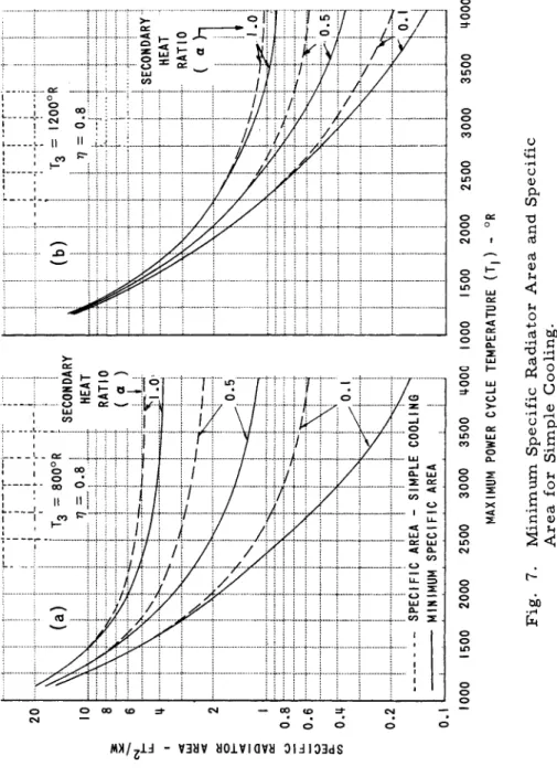
In Fig. 7, the minimum specific radiator area and the spe­

cific area required for simple cooling are plotted against max­

imum power cycle temperature for the indicated values of 7) and T3. When T 3 = 800°R, the minimum specific area is not noticeably less than that for simple cooling until Tj exceeds

1600°R. When T 3 = 1200°R, the minimum specific area is not noticeably less than that for simple cooling until Tj ex­

ceeds 2400°R. These observations confirm an earlier conclu­

sion that simple cooling is the p r e f e r r e d mode when β(Τ$/T\) >

0.5.

Real Cycle Analysis

The analysis of specific radiator area previously described has been carried out using ideal working fluids in the Carnot and reversed Carnot cycles, modified to allow for inefficiencies

151

Fig. 7. Minimum Specific Radiator Area and Specific Area for Simple Cooling.

152

in the expansion and compression processes. Now the anal­

ysis will be repeated using the Rankine vapor cycle and real fluids.

Fig. 8 shows Rankine thermodynamic cycles for the power plant working fluid and the secondary coolant, modified to al­

low for inefficiencies in the expansion and compression proc­

esses. A single secondary waste source is assumed. Only compression of the coolant prior to waste heat rejection in the secondary radiator is considered, since the analysis thus far presented has shown that expansion of the secondary coolant prior to entering the secondary radiator produces a relatively

small reduction in radiator area.

In Fig. 8A, saturated vapor at a expands through a tur­

bine with efficiency 7]^ to b ' . The vapor condenses while flowing through the p r i m a r y radiator, moving from b' to c.

The saturated liquid at c is pumped to higher p r e s s u r e at c, becoming subcooled prior to entering the heat source. (Pump­

ing power is assumed to be negligible.) The subcooled liquid is then heated at constant p r e s s u r e , and moves successively to points d and a, completing the cycle. It is assumed that the working fluid temperature remains constant at T 2 as the state point of expanded vapor passes from b! to c, even if b should lie to the right of the saturated vapor line.*

In Fig. 8 B , the secondary coolant at point f is compressed with an efficiency rj^s to point j ' . The coolant then enters the secondary radiator, via path j ' - j - k , giving up its accumulated heat. Upon leaving the radiator, the coolant expands in a throt­

tling (constant enthalpy) process to point e', and then moves to point f as heat is accumulated from the secondary heat source, completing the cycle. The fluid undergoes the throttling proc­

ess between k and e¹ because relatively little work is obtain­

able under even the most ideal expansion process k-e". It is assumed that as the coolant loses heat in the radiator its tem­

perature remains constant at T4, although the temperature at j^! is greater than T4.1

*If point b' lies to the right of the saturated vapor line, the mean temperature of the working fluid in the radiator will ex­

ceed T2, and the specific radiator area will be less than if the working fluid temperature w e r e always T£. However, the difference in specific area will be relatively small, since generally only a small fraction of the total heat content of the working fluid will be associated with the superheated state.

fThe influence of this assumption on specific a r e a will be r e l a ­ tively small for the same reasons as advanced in the previous footnote.

155

1⁵4

Fig. 8A. Real Power Cycle . Fig. 8B. Real Secondary Coolan

A s was done for the ideal cycle analysis, expressions can be obtained for the p r i m a r y radiator area A , the secondary radiator a, and the secondary coolant cycle work w in terms of the generated power W in the power cycle. If these ex­

pressions are substituted into Eq. (1), the dimensionless spe­

cific radiator area φ* for real fluid s is found to be:

Ψ -

(8*-D

, (8*

's

8

Eq. (12) is identical in form to Eq. (4) for φ, the dimensionless specific area for an ideal working fluid.

φ⁰* and 8* have the same physical significance as φ⁰ and 8 in the ideal cycle analysis, but are expressed in terms of enthalpy rather than temperature. φ0* and φ0 represent the dimensionless specific radiator area when secondary waste heat is not present. 8* and 8 are the ratios of heat rejected from the secondary radiator, following isentropic compression of the secondary coolant, to heat added to the secondary cool­

ant.

It can be shown that

* 1 - *7^t<l - pr)

Φ⁰ = - - τ <¹³>

where

R - I N R

Ρ = Ρ , + 1 - τ (1 4>

and Pi is Mackey's fluid parameter h f g i /C \ T \ · hfgi is the heat of vaporization at Ti, and C l is the mean specific heat of the liquid working fluid between the maximum power cycle temperature T\ and the heat rejection temperature Τ;*.

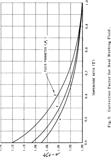
A plot of ρ as a function of Pi and τ is given in Fig. 9.

When P[ > 2 and 0.7 < τ < 1.0, 1.00 £ ρ < 1.02. A s Pi ap­

proaches infinity, ρ approaches unity, and the real cycle b e ­ comes identical with the ideal cycle.

To find , the value of τ for which φ⁰* is a minimum, Eq. (13) must be differentiated with respect to r. The differ­

entiation is simplified if ρ is assumed to be constant. As in­

dicated above, the assumption will not introduce serious error if 0.7 < r^m^ 1 . 0 and Pi ^- 2. The latter condition is charac­

teristic of liquid metal working fluids.

155

156

Fig. 9. Correction Factor for Real Working Fluid.

Upon performing the differentiation on the assumption that ρ is constant and solving for , it is found that

m (15)

where T ^{M ?} defined by Eq. (7), is the optimum temperature ratio for an ideal fluid. F o r the same maximum power cycle temperature T j , it is evident from Eq. (15) that ρ is the ratio of optimum heat rejection temperatures in the ideal and real cycles. If is substituted for τ in Eq. (13), it can be shown that

om ρ < f t ο m (16) where <£om ^^s the mjnimum dimensionless specific area for an ideal fluid, and < £ ô^m represents the same quantity for a real (liquid metal) working fluid. The ratio of minimum p r i - mary radiator areas for real and ideal fluids is thus equal to

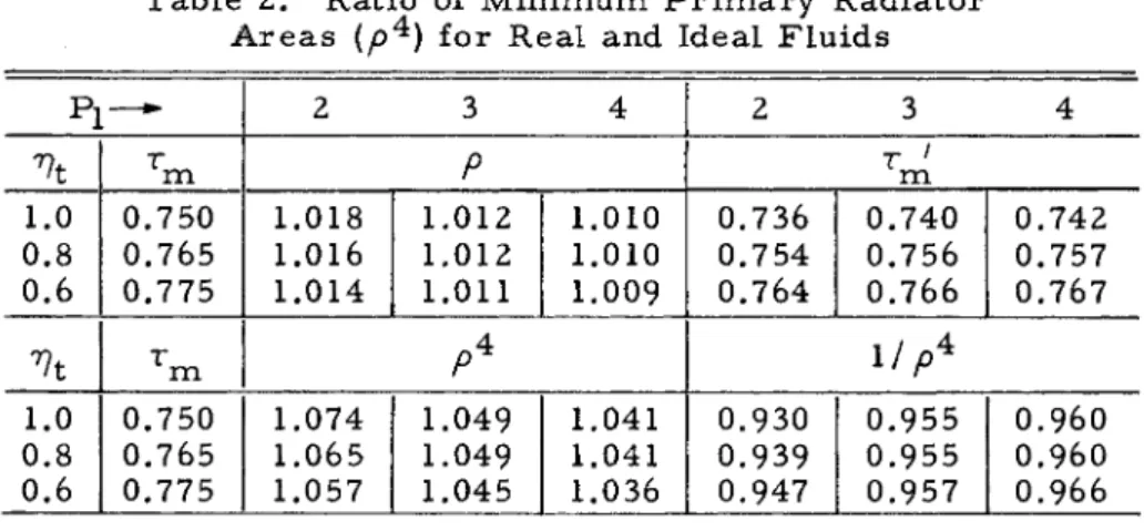
Table 2 shows how p^ varies with the fluid parameter Pi and the temperature ratio

Table 2. Ratio of Minimum P r i m a r y Radiator A r e a s (p^) for Real and Ideal Fluids

P i — 2 3 4 2 3 4

v^t Tm Ρ Trri

1.0 m 0.8 0.6

0.750 0.765 0.775

1.018 1.016 1.014

1.012 1.012 1.011

1.010 1.010 1.009

0.736 0.754 0.764

0.740 0.756 0.766

0.742 0.757 0.767

Vt ^Tm Ρ⁴ H P 4

0.8 1.0 0.6

0.750 0.765 0.775

1.074 1.065 1.057

1.049 1.049 1.045

1.041 1.041 1.036

0.930 0.939 0.947

0.955 0.955 0.957

0.960 0.960 0.966 F r o m the values of Y O⁴ in Table 2, it can be seen that the minimum radiator area is greater for the real cycle, but by a relatively small percentage. Also, 0.7 < TM' < 1.0, validating the assumption made above about p. F o r the range of v a r i ­ ables shown in Table 2, use of the ideal cycle underestimates the area of the p r i m a r y radiator by between 3 and 7%. F u r ­ ther, this range of e r r o r is valid for real fluids, such as liquid metals, with a value of the fluid parameter P^ as low as two.

157

n =

P

+

+ InS

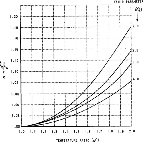
and P4 is the fluid parameter h£ 4/ C4T4.

For the same rate of secondary waste heat production, η is just the ratio of heat rejection rates in the reversed Rankine and reversed Carnot cycles. Eq. (18) is plotted in Fig. 10.

The heat rejection ratio η is seen to increase with δ and de­

crease with P4. As P4 approaches infinity, η approaches unity, and the reversed real cycle becomes identical with the reversed ideal cycle.

The results obtained above for real fluids readily apply to the case of secondary waste heat removal by simple cooling if δ is given the value of one. In this instance η also is ecniai to one, as is evident from Eq. (18). Then Eq. (12) for φ b e ­ comes:

The ratio of radiator areas for real and ideal fluids with simple cooling is φι Iφ\.

Using E q s . (2) and (19),

Φ* _{sl. + α}

Φι ' 1

(20)

If the minimum values of </>^Q* and φ⁰ are used, then E q s . (6) and (16) may be employed to show that

Φι ^{= 1 + (21)}

158

F L U I D PARAMETER

1 . 0 I . I 1 . 2 1 . 3 I Λ 1 . 5 1 . 6 1 . 7 1 . 8 1 . 9 2 . 0

T E M P E R A T U R E R A T I O ((f)

Fig. 10. Correction Factor for Real Secondary Coolant.

159

om Using Eq. (19) with φ⁰* = φ

ôm a n (^ Eq. (16) and (6), it may be shown that

* F

F (23) Thus, for simple cooling the fractional increase in radiator

area for real fluids is equal to that for an ideal fluid divided by p^. Values of 1/p^ are given in Table 2.

Comparison of Real and Ideal Cycles

Using the expressions obtained for p^ = and η = δ * / δ , the dimensionless specific area for real fluids φ*

may be calculated f r o m Eq. (12) and the results compared with the results of the ideal fluid analysis. In order to find the value of δ which minimizes φ*, Eq. (12) can be differentiated with respect to δ and then set equal to zero, or alternatively, φ* can be plotted against δ for various values of the p a r a m ­ eters a , p^y and Tj. Because of the complexity of the differ­

entiated equation, the latter course was followed.

Curves were constructed for values of β varying from 0,2 to 0.6, which is the range of greatest practical interest.

A value of 2.0 was chosen for both and P 4 . This value is less than that for liquid metals in the temperature range of interest.Î Since, as Ρ increases, the discrepancy between real and ideal fluids grows smaller, calculations with Ρ = 2.0 should give an upper limit on the difference in radiator char­

acteristics between a system employing an ideal fluid and one employing liquid metals.

F r o m the curves of φ* vs δ , the optimum temperature ratio δ ^ and the minimum radiator area ratio R ^ -φ^/φοτη for real fluids can be obtained. Minimum area ratios obtained in this manner are shown as dashed lines in Fig. 4 .

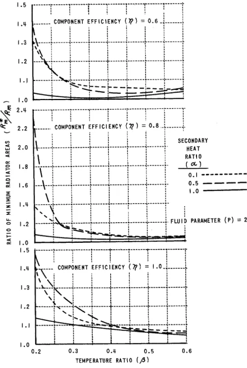
In Fig. 11, the ratio of the minimum radiator areas for real and ideal fluids, RI* / Rm =

Ψηι^πυ

tion of the temperature ratio /3, the secondary heat ratio a , tSee Fig. 3, Ref. 2.

160

I . 5

I Λ

1.3

1 . 2

I.J

I . 0

2Λ

2 . 2

2 . 0

1 . 8

1 . 6

I Λ

I . 2

COMPONENT E F F I C I E N C Y ( T? ) = [ ' ! ! ! ! !

» ! ! !

Λ [ ! . i J . ! !

0 . 6 _.

T " \ ^!

v

\ 1

Η ' _i ' i_ '

\ I I

• V . L j L !

Γ jHrzrbrL-

1

|r

I

1 1

COMPO NENT Ε F F I C I ENCY ( 9 ? ) = 0.8.„L

ι

. . .

\

\

. . .

\

S E C O N D A R Y H E A T R A T I O

( 0 . 1 0 . 5 1 . 0

F L U I D P A R A M E T E R ( P )

0 . 2 0 . 3 OA ^{0 . 5}

T E M P E R A T U R E R A T I O (β)

0 . 6

Fig. 1 1 . Ratio of Minimum Radiator A r e a s for Real and Ideal Fluids.

161

ideal fluids occurs when 0.1 < Ct < 1,0,

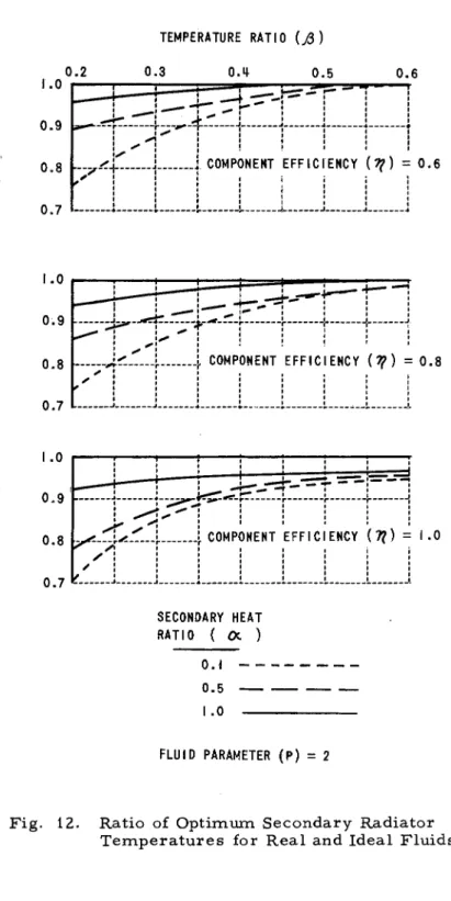
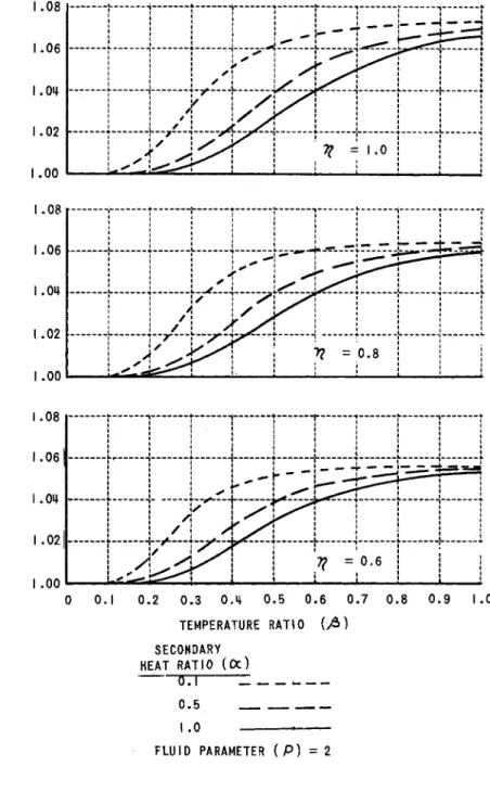
The dependence of the ratio 8^m7 S ^m on /3, a , and Ύ) is shown in Fig. 12. For the same secondary waste heat temper­

ature, SrnV O ^m is the ratio of secondary radiator tempera­

tures for real and ideal fluids. It can be seen that the opti­

mum secondary radiator temperature for a real fluid is less than for the ideal fluid, and becomes increasingly so as β and Ct grow smaller and rj grows l a r g e r .

When β > 0. 5 , as has been pointed out in describing the ideal fluid analysis, the radiator area required for an ideal fluid in the simple cooling mode (8 = 1 ), is at most 10% greater than the minimum radiator a r e a , which is attained when δ < 1.

Therefore, the simple cooling mode can be used for an approx­

imate determination of radiator a r e a when β > 0.6. The ratio of radiator area for real fluids ( P = 2.0) to that for an ideal fluid is shown in Fig. 13 for the simple cooling mode, i. e. , when 8 = 1. It can be seen that the radiator area is l a r g e r for the real fluid, increasing as β grows l a r g e r and α grows

smaller. The maximum difference is 7.3%, which occurs when η = 1.0, α = 0.1, and β = 1.0.

F r o m the above discussion, it may be concluded that when β > 0.3, the radiator a r e a calculated f r o m the ideal fluid anal­

ysis is a reasonable first approximation to the radiator a r e a for liquid metal working fluids and secondary coolants. When 0.3 < /3.< 0.6, the ideal fluid analysis predicts radiator areas which are too low by 20% or less. When 0.6 < β < 1.0 and the simple cooling mode for secondary waste heat removal is a s ­ sumed, the radiator area predicted by the ideal fluid analysis is too low by about 7% or less. The radiator area calculated from the ideal fluid analysis will in general differ from the radiator a r e a for real fluids by less than the maximum p e r ­ centages indicated above.

ΐφιη/φοηι is the ratio of the minimum radiator area for real fluids for a specified α to the minimum radiator a r e a for an an ideal fluid when α = 0.

<£m7<£

162

TEMPERATURE RATIO (β)

0 . 2 0 . 3 0Λ 0 . 5 0 . 6

SECONDARY HEAT RATIQ ( α )

0 . 1

I . 0

FLUID PARAMETER ( P ) = 2

Fig. 12. Ratio of Optimum Secondary Radiator Temperatures for Real and Ideal Fluids.

16?

1 . 0 0 I :

J T ,

< : I ; S

— — 1 — — - - • { 1

! 1 ! Ι , ι

~ ~

•

i - " Γ L — —

Ό^ Ι Ί

~ ' ϊ

S J { Ι Ι ! Ι !

• !

„ .L . 1

y / 1 7? = 0 . 6

r ι i ^I

" Ι — *

\ ! ι ; I ;

Ο 0 . 1 0 . 2 0 . 3 Ο Λ 0 . 5 0 . 6 0 . 7 0 . 8 0 . 9 1.0 T E M P E R A T U R E R A T I O ( A )

SECONDARY HEAT R A T I O ( A )

— ~ ϋ π ^{Ζ .}

1.0 · —

F L U I D PARAMETER ( P ) = 2

Fig. 13. Ratio of Radiator A r e a s for Real and Ideal Fluids When Simple Cooling is Used.

164

Illustrative Example

To illustrate how the information developed in this paper can be used to estimate the radiator area of space power plants, the following example is presented.

Consider a space power plant using rubidium* as the work­

ing fluid in the Rankine thermodynamic cycle and as the cool­

ant for the removal of secondary waste heat. The maximum temperature of the power cycle is 2000°R. Fifty percent of the shaft power generated is dissipated as secondary waste heat in the electrical load. The maximum permissible tem­

perature of components comprising the electrical load is 1000eR.

The efficiency of expansion or compression of rubidium vapor is 80%. The emissivity of the radiator surface is 0.8.

Assuming that rubidium is an ideal fluid, find

1) The minimum specific radiator area for rejection of waste heat f r o m the power cycle alone.

2) Optimum mode for secondary waste heat removal.

3) The minimum specific radiator area for rejection of both power cycle heat and secondary waste heat, and the temperature of the secondary radiator.

4) Specific radiator area when secondary waste heat is removed by simple cooling.

5) Adequacy of ideal fluid assumption.

Solution: F r o m information given in the statement of the problem, the basic input is:

Τι = 2000*R T³ = 1000^eR

η = 0.8

€ = 0.8 a = 0.5

1. F r o m E q . ( l A ) , A / W = φ0/€ σ"Τ14· F r o m Table 1, < £^{o m} = 12.63.

Using the value of 1713 χ 10-12 B t u / h r - f t²-^eR⁴ for the Stefan-Boltzmann constant cr^? crT]4 = 8.0 kw/ft^. Thus, A / W = 12.63/0.8(8.0) = 1.97 f t²/ k w .

2. By definition, β = T3/Τχ = 0.5.

F r o m Fig. 3, $i = 0.60.

Since β < , compression of the secondary coolantprior to entering the radiator is the optimum mode for removal of

secondary waste heat.

3. F r o m E q . ( l ) , ( A + a ) / ( W + w ) = φ/^σ-Τχ⁴.

F r o m Fig. 4B, R ^m = 1.58. Also, </>^m = < / >^{o m}R^m

= 12.63 (1.58) = 20.0.

Thus,(A + a ) / ( W + w ) = 20.0/0.8(8.0) = 3.12 f t²/ k w . F r o m Fig. 3B, 8^m = T 4 / T 3 = 1.16.

# Rubidium is considered as a possible working fluid for space power plants in Réf. 1.

I65

than that for simple cooling.

5. F r o m Fig. 3 of Ref. 2, Ρχ is about 2 and P 4 is about 3.6.

If it is assumed that both Ρχ and P 4 are equal to 2, the maxi­

mum deviation of the ideal fluid analysis from that of real fluids will be obtained, since the deviation increases as Ρ de­

creases. F r o m Fig. 11, < £^m/φ^{τ η} = 1.05. Thus, the radiator area for the real working fluid is at most 5% greater than that for the ideal fluid.

Conclusions

The production of secondary waste heat aboard spacecraft (waste heat from processes other than the inefficient conver­

sion of thermal energy to some other form) can result in a significant increase in radiator area when (1) the secondary waste heat production rate is a significant fraction of gener­

ated power, and (2) the temperature of the component in which secondary waste heat appears is small compared to the maxi­

mum power cycle temperature.

Secondary waste heat may be rejected by simple cooling followed by direct transfer of the coolant to a secondary radi­

ator, or by expansion or compression of the coolant prior to entering the radiator. The optimum cooling mode is deter­

mined primarily by β, the ratio of the secondary heat source temperature to the maximum power cycle temperature. When

β exceeds 0.5, simple cooling is preferred. When β is less than 0.5, either simple cooling or prior compression of the coolant is preferred, depending on the magnitude of rj , the compressor or turbine efficiency, and a , the ratio of second­

ary waste heat production to generated power.

Within the range of operating conditions for which sec­

ondary waste heat significantly influences radiator area, an increase in the permissible temperature of components in which secondary heat is produced and/or a reduction of the secondary heat production rate may be more effective in r e ­ ducing radiator area than an increase in the maximum power cycle temperature.

Within the range of operating conditions for which most of the radiator area is determined principally by the rejection of

secondary heat, optimization of the p r i m a r y radiator area has 166

relatively little effect on total radiator area. F o r these con­

ditions, other considerations may become dominant, such as efficiency of thermal energy conversion or design of the ther­

mal energy source.

Use of an ideal fluid rather than a real cycle working fluid results in an underestimate of radiator area. When β^

0.3, the ideal fluid analysis results in a radiator area which is 20% or less below that required for liquid metal fluids.

When β > 0.4, the er ror resulting from use of the ideal fluid analysis is 10% or less.

Nomenclatur e

= maximum absolute temperature of power cycle

= absolute temperature of p r i m a r y radiator = min­

imum absolute temperature of power cycle

= absolute temperature of secondary waste heat source

= absolute temperature of secondary radiator W = power generated in power cycle

A = p r i m a r y radiator area needed to generate W units of power

w = power to compress secondary coolant or power produced by secondary coolant

a = secondary radiator area needed to generate W units of power

a = secondary heat ratio = ratio of secondary waste heat production rate to generated power W S = entropy

7f^ = expansion efficiency in power cycle

r) = expansion or compression efficiency in second­

ary coolant cycle

7} = component efficiency = rj^ = rj^

(T = Stefan-Boltzmann constant

€ = radiator emissivity C = specific heat of liquid h^g = heat of vaporization

Ρ = fluid parameter = h^{f r Y}/ CT

167

τ = ratio of heat rejected to heat added in ideal power cycle

δ = ratio of heat rejected to heat added in ideal sec­

ondary coolant cycle

φ = dimensionless specific radiator area for ideal fluid

φ^ = φ when secondary waste heat is negligible R = for ideal fluid, ratio of radiator areas with and

without secondary waste heat = φ/φ^ or φ / Φ^{ο τ η} F = for ideal fluid, ratio of increase in radiator area

with secondary waste heat and simple cooling to radiator area without waste heat

ρ = τ / τ ' = ratio of heat rejection rates in Rankine and Carnot cycles

η = δ * / δ = ratio of heat rejection rates in reversed Rankine and reversed Carnot cycles

Subscript "m" — denotes minimum value or optimum value Subscript "1" — denotes secondary waste heat removal by

simple cooling Superscript "1" — denotes real fluid

Superscript "*" — denotes real fluid or Rankine cycle References

1. Mackey, D. Β. , "Powerplant Heat Cycles for Space Vehi­

cles," IAS Paper No. 59-104. Presented at IAS National Summer Meeting, June 16-19, 1959, Los Angeles, Calif.

2. Mackey, D. Β. , "Secondary Power Systems for Space Vehi­

cles," for presentation at the Society of Automotive Engi­

neers, National Aeronautic Meeting, October 10-14, I960, Los Angeles, Calif.

3. English, R. Ε. , jet al, " A 20,000 Kilowatt Nuclear Turbo- electric Power Supply for Manned Space Vehicles," Memo 2-20-59E, National Aeronautics and Space Administration, Washington, March 1959.

168

I69

Moffitt, T . P . , and Klag, F. W . , "Analytical Investigation of Cycle Characteristics for Advanced Turboelectric Space Power Systems," N A S A T N D-472, National Aeronautics and Space Administration, Washington, October I960.

Fisher, J . H . , and Stéphane, C. W . , "Basic Energy Con­

version in Space Vehicles," presented at American Rocket Society 14th Annual Meeting, November 16-20, 1959, Washington, D. C.

Macklin, Μ . , "Space Cooling P r o c e d u r e s , " IAS Paper 61- 18, presented at the IAS 29th Annual Meeting, New York, January 23, 1961.