1 The interplay of landscape composition and configuration: new pathways to manage 1
functional biodiversity and agro-ecosystem services across Europe 2
3
Emily A. Martin1*, Matteo Dainese2, Yann Clough3, András Báldi4, Riccardo Bommarco5, 4
Vesna Gagic6, Michael Garratt7, Andrea Holzschuh1, David Kleijn8, Anikó Kovács- 5
Hostyánszki4, Lorenzo Marini9, Simon G. Potts7, Henrik Smith3, Diab Al Hassan10, Matthias 6
Albrecht11, Georg K.S. Andersson3, Josep D. Asís12, Stéphanie Aviron13, Mario Balzan14, 7
Laura Baños-Picón12, Ignasi Bartomeus15, Péter Batáry16, Francoise Burel10, Berta Caballero- 8
López17, Elena D. Concepción18, Valérie Coudrain19, Juliana Dänhardt3, Mario Diaz18, Tim 9
Diekötter20, Carsten F. Dormann21, Rémi Duflot22, Martin H. Entling23, Nina Farwig24, 10
Christina Fischer25, Thomas Frank26, Lucas A. Garibaldi27, John Hermann20, Felix Herzog11, 11
Diego Inclán28, Katja Jacot11, Frank Jauker29, Philippe Jeanneret11, Marina Kaiser30, Jochen 12
Krauss1, Violette Le Féon31, Jon Marshall32, Anna-Camilla Moonen33, Gerardo Moreno34, 13
Verena Riedinger1, Maj Rundlöf35, Adrien Rusch36, Jeroen Scheper37, Gudrun Schneider1, 14
Christof Schüepp38, Sonja Stutz39, Louis Sutter11, Giovanni Tamburini5, Carsten Thies40, José 15
Tormos12, Teja Tscharntke41, Matthias Tschumi11, Deniz Uzman42, Christian Wagner43, 16
Muhammad Zubair-Anjum44, Ingolf Steffan-Dewenter1 17
18
1 Animal Ecology and Tropical Biology, Biocenter, University of Würzburg, Am Hubland, 19
97074 Würzburg, Germany 20
2 Institute for Alpine Environment, EURAC Research, Viale Druso 1, 39100 Bolzano, Italy 21
3 Centre for Environmental and Climate Research, Lund University, 22362, Lund, Sweden 22
4 MTA Centre for Ecological Research, Institute for Ecology and Botany, Lendület Ecosystem 23
Services Research Group, Alkotmány u. 2-4, 2163 Vácrátót, Hungary 24
5 Department of Ecology, Swedish University of Agricultural Sciences, SE-750 07 Uppsala, 25
Sweden 26
6 Commonwealth Scientific and Industrial Research Organisation, Dutton Park, Queensland, 27
Australia 28
7 Centre for Agri-Environmental Research, School of Agriculture, Policy and Development, 29
Reading University, RG6 6AR, UK 30
8 Plant Ecology and Nature Conservation Group, Wageningen University, Droevendaalsesteeg 31
3, 6708PB Wageningen, The Netherlands 32
2
9 DAFNAE, University of Padova, Viale dell’Università 16, 35020 Legnaro (Padova), Italy 33
10 UMR 6553 Ecobio, CNRS, Université de Rennes 1, Campus de Beaulieu, 35042 Rennes 34
Cedex, France 35
11 Agroecology and Environment, Agroscope, Reckenholzstrasse 191, 8046 Zurich, 36
Switzerland 37
12 Departamento de Biología Animal (Área de Zoología), Facultad de Biología, Universidad 38
de Salamanca, Campus Miguel de Unamuno s/n, 37007 Salamanca, Spain 39
13 UMR BAGAP - INRA, Agrocampus Ouest, ESA, 49000 Angers, France 40
14 Institute of Applied Sciences, Malta College of Arts, Science and Technology (MCAST), 41
Paola, Malta 42
15 Estación Biológica de Doñana (EBD-CSIC). E-41092 Sevilla, Spain 43
16 MTA ÖK Lendület Landscape and Conservation Ecology Research Group, Alkotmány u. 2- 44
4, 2163 Vácrátót, Hungary 45
17 Department of Arthropods, Natural Sciences Museum of Barcelona, Castell dels Tres 46
Dragons, Picasso Av, 08003 Barcelona, Spain 47
18 Department of Biogeography and Global Change, National Museum of Natural Sciences, 48
Spanish National Research Council (BGC-MNCN-CSIC), C/ Serrano 115 bis, E-28006 49
Madrid, Spain 50
19 Mediterranean Institute of Marine and Terrestrial Biodiversity and Ecology (IMBE), Aix- 51
Marseille University, CNRS, IRD, Univ. Avignon, 13545 Aix-en-Provence, France 52
20 Department of Landscape Ecology, Kiel University, Olshausenstrasse 75, 24118 Kiel, 53
Germany 54
21 Biometry & Environmental System Analysis, University of Freiburg, Germany 55
22 Department of Biological and Environmental Sciences, University of Jyväskylä, Finland 56
23 Institute for Environmental Sciences, University of Koblenz-Landau, Fortstr. 7, 76829 57
Landau, Germany 58
24 Department of Conservation Ecology, Faculty of Biology, Philipps-University Marburg, 59
Karl-von-Frisch Str. 8, 35043 Marburg, Germany 60
25 Restoration Ecology, Department of Ecology and Ecosystem Management, Technische 61
Universität München, 85354 Freising, Germany 62
26 University of Natural Resources and Life Sciences, Department of Integrative Biology and 63
Biodiversity Research, Institute of Zoology, Gregor Mendel Straße 33, A-1180 Vienna, 64
Austria 65
3
27 Instituto de Investigaciones en Recursos Naturales, Agroecología y Desarrollo Rural 66
(IRNAD), Sede Andina, Universidad Nacional de Río Negro (UNRN) and Consejo Nacional 67
de Investigaciones Científicas y Técnicas (CONICET), Mitre 630, CP 8400, San Carlos de 68
Bariloche, Río Negro, Argentina 69
28 Instituto Nacional de Biodiversidad, INABIO – Facultad de Ciencias Agícolas, Universidad 70
Central del Ecuador, Quito 170129, Ecuador 71
29 Department of Animal Ecology, Justus Liebig University, Heinrich-Buff-Ring 26-32, D- 72
35392 Giessen, Germany 73
30 Faculty of Biology, Institute of Zoology, University of Belgrade, Studentski trg 16, 74
Belgrade 11 000, Serbia 75
31 INRA, UR 406 Abeilles et Environnement, Site Agroparc, 84914 Avignon, France 76
32 Marshall Agroecology Ltd, Winscombe, UK 77
33 Institute of Life Sciences, Scuola Superiore Sant’Anna, Piazza Martiri della Libertà 33, I- 78
56127 Pisa, Italy 79
34 INDEHESA, Forestry School, Universidad de Extremadura, Plasencia 10600, Spain 80
35 Department of Biology, Lund University, 223 62 Lund, Sweden 81
36 INRA, UMR 1065 SAVE, ISVV, Université de Bordeaux, Bordeaux Sciences Agro, F- 82
33883 Villenave d’Ornon, France 83
37 Animal Ecology Team, Wageningen Environmental Research, Droevendaalsesteeg 3, 6708 84
PB Wageningen, The Netherlands 85
38 Institute of Ecology and Evolution, University of Bern, CH-3012 Bern, Switzerland 86
39 CABI, Rue des Grillons 1, 2800 Delémont, Switzerland 87
40 Natural Resources Research Laboratory, Bremer Str. 15, 29308 Winsen, Germany 88
41 Agroecology, University of Göttingen, Grisebachstrasse 6, 37077 Göttingen, Germany 89
42 Department of Crop Protection, Geisenheim University, Von-Lade-Str. 1, 65366 90
Geisenheim, Germany 91
43 LfL, Bayerische Landesanstalt für Landwirtschaft, Institut für Ökologischen Landbau, 92
Bodenkultur und Ressourcenschutz, Lange Point 12, 85354 Freising, Germany 93
44 Department of Zoology & Biology, Faculty of Sciences, Pir Mehr Ali Shah Arid 94
Agriculture University Rawalpindi, Pakistan 95
96
* Corresponding author: email: emily.martin@uni-wuerzburg.de, phone: +499313183876.
97 98
4 Article type: Letter
99 100
Author contributions: EAM, ISD, MD, YC, AB, RB, VG, MG, AH, DK, AK, LM, SP, HS 101
designed the study. DAH, SA, MA, GKSA, MAZ, JDA, AB, MB, LBP, IB, PB, RB, FB, 102
BCL, YC, EDC, VC, MD, JD, MDíaz, TD, CFD, RD, MHE, NF, CF, TF, VG, LAG, MG, JH, 103
FH, AH, DI, KJ, FJ, PJ, MK, DK, AKH, JK, VLF, LM, JM, ACM, GM, SP, VR, MR, AR, 104
JS, GS, CS, HS, ISD, SS, LS, GT, CT, JT, TT, MT, DU, CW performed the research. EAM 105
analyzed the data. EAM, ISD, MD, YC interpreted results. EAM wrote the paper and all 106
authors contributed substantially to revisions.
107 108
Data accessibility: Should the manuscript be accepted, the data supporting the results will be 109
archived in an appropriate public repository such as Dryad or Figshare and the data DOI will 110
be included at the end of the article 111
112
Word count: Abstract 150 words, main text 5,000 words, 67 references, 4 figures, 1 table.
113 114
Keywords: Agroecology, arthropod community, biological control, edge density, pest control, 115
pollination, response trait, semi-natural habitat, trait syndrome, yield.
116 117 118 119 120 121 122 123
5 Abstract
124
Managing agricultural landscapes to support biodiversity and ecosystem services are key aims 125
of a sustainable agriculture. However, how the spatial arrangement of crop fields and other 126
habitats in landscapes impacts arthropods and their functions is poorly known. Synthesizing 127
data from 49 studies (1,515 landscapes) across Europe, we examined effects of landscape 128
composition (% habitats) and configuration (edge density) on arthropods in fields and their 129
margins, pest control, pollination and yields. Configuration effects interacted with proportions 130
of crop and non-crop habitats, and species’ dietary, dispersal and overwintering traits led to 131
contrasting responses to landscape variables. Overall, however, in landscapes with high edge 132
density, 70% of pollinator and 44% of natural enemy species reached highest abundances and 133
pollination and pest control improved 1.7 and 1.4-fold, respectively. Arable-dominated 134
landscapes with high edge densities achieved high yields. This suggests that enhancing edge 135
density in European agroecosystems can promote functional biodiversity and yield-enhancing 136
ecosystem services.
137 138 139 140 141 142 143 144 145
6 INTRODUCTION
146
Worldwide, intensive agriculture threatens biodiversity and biodiversity-related ecosystem 147
services (Foley et al. 2005). At a local field scale, monocultures and pesticides restrict many 148
arthropods and plants to non-cropped areas (Geiger et al. 2010). Thus, the majority of 149
organisms that provide key regulating services to agriculture, such as pollination and natural 150
pest control, must colonize fields from non-cropped, semi-natural areas (e.g. road verges, 151
grass margins, hedgerows, fallows), neighboring fields or in the wider landscape (Blitzer et 152
al. 2012). Semi-natural habitats, however, are often removed to facilitate the use of modern 153
machinery or converted to crops to increase production (Naylor & Ehrlich 1997), resulting in 154
reduced populations of service providing organisms (Holland et al. 2016). Consequently, the 155
sustainability of modern food production is increasingly questioned (Garnett et al. 2013).
156
‘Ecological intensification’ has the potential to enhance the sustainability of agricultural 157
production by increasing the benefits agriculture derives from ecosystem services (Bommarco 158
et al. 2013). Supporting populations of ecosystem service providers is a key component of 159
ecological intensification (Bommarco et al. 2013). However, we currently lack detailed 160
knowledge on the landscape-scale management choices needed to achieve ecological 161
intensification with a high degree of certainty (Kleijn et al. 2019). For example, semi-natural 162
habitats are prerequisite for many organisms, but effects are often taxon-specific. In addition, 163
the presence or abundance of functional groups of organisms in a landscape does not always 164
correlate with the services they provide to crops (Tscharntke et al. 2016; Karp et al. 2018).
165
The configuration of landscapes (size, shape and spatial arrangement of land-use patches), in 166
addition to their composition (proportion of land-use types), is increasingly suggested as a key 167
factor in determining biodiversity and associated ecosystem services in agricultural 168
landscapes (Fahrig 2013). However, studies have only begun to disentangle the relative roles 169
7 of the composition vs. the configuration of habitats and fields within landscapes (Fig. 1;
170
Fahrig 2013; Haddad et al. 2017). Landscape configuration can be measured as the density of 171
edges between crop fields and their surroundings, including neighboring crops and non-crop 172
areas. Complex landscapes where small and/or irregularly shaped fields and habitat patches 173
prevail have a high density of edges. Due to increased opportunities for exchange, these 174
landscapes are likely to support spillover of dispersal-limited populations between patches 175
(Smith et al. 2014; Fahrig 2017). This may enhance populations’ survival in the face of 176
disturbance and their potential to provide services in crops (Boetzl et al. 2019). Further, if 177
landscapes with high edge density are also spatially and temporally diverse in their 178
composition, organisms in these landscapes may benefit from landscape-scale resource 179
complementation and supplementation (Dunning et al. 1992). In this context, areas offering 180
refuges or complementary food resources may encompass uncropped (semi-natural) areas, but 181
also neighboring crops with asynchronous phenology, different host species and/or variable 182
timing and intensity of management interventions (Vasseur et al. 2013; Schellhorn et al.
183
2015). However, previous studies have found contrasting effects of increasing configurational 184
complexity for different taxa (Concepción et al. 2012; Plećaš et al. 2014; Duflot et al. 2015;
185
Fahrig et al. 2015; Gámez-Virués et al. 2015; Perović et al. 2015; Martin et al. 2016; Bosem 186
Baillod et al. 2017; Hass et al. 2018). Thus, there is currently no consensus on the importance 187
of landscape configuration for arthropods and the services they provide in crops (Seppelt et 188
al. 2016; Perović et al. 2018). Further, interactions between landscape composition and 189
configuration might explain seemingly contradictory results, but have rarely been tested in 190
part due to a lack of independent landscape gradients (but see Coudrain et al. 2014; Bosem 191
Baillod et al. 2017).
192
Species’ responses to environmental filters depend on sets of biological traits (‘response 193
traits’), such as diet breadth and dispersal ability, that constrain species’ reactions to 194
8 environmental predictors (Lavorel & Garnier 2002). The resulting filtering of ecological 195
communities determines the presence or abundance of arthropods able to provide ecosystem 196
services (Gámez-Virués et al. 2015). Organisms with similar responses to environmental 197
filters may share specific combinations of response traits, known as trait syndromes.
198
Characterizing these syndromes and their responses to landscape gradients is critical to 199
predict the consequences of land-use change for biological communities (Mouillot et al.
200
2013) and the services they provide. However, trait-based responses of arthropods in cropland 201
to landscape gradients have only recently been investigated (Bartomeus et al. 2018; Perović et 202
al. 2018) and cross-taxonomic approaches in agroecosystems are lacking (but see Gámez- 203
Virués et al. 2015). For pollinators, natural enemies and pests in agricultural landscapes, a 204
high diversity of responses due to trait variation within and between groups (‘response 205
diversity’) is likely to underlie observed abundance patterns. In turn, this may affect our 206
ability to manage landscapes for maximum abundance and/or effectiveness of crop ecosystem 207
service-providers, and for minimum impacts of pests.
208
Here, using data from 49 studies covering 1,515 European agricultural landscapes and more 209
than 15 crops, we aim to disentangle arthropod responses to landscape gradients and their 210
consequences for agricultural production by performing the first empirical quantitative 211
synthesis of the effects of landscape configuration (edge density) and composition (amount of 212
crop and semi-natural habitats) on arthropods and their services in cropland. We include 213
observations of the abundance of pollinators, pests and pests’ natural enemies (predators and 214
parasitoids) sampled in fields and their margins, and measures of natural pest control, 215
pollination, and crop yields. We use landscape predictors calculated similarly for all studies 216
from high resolution maps with standard land use-land cover classification. We test the 217
following predictions:
218
9 1. Within functional groups of pollinators, pests and natural enemies, responses to landscape 219
predictors differ among trait syndromes. Thus, considering key trait syndromes of arthropods 220
should increase our ability to predict the effects of landscape variables on functional groups.
221
On one hand, species that use specific crop or non-crop resources should benefit from 222
increased proportions of these resources (habitats) in the landscape (Tscharntke et al. 2012).
223
On the other hand, species with medium to low dispersal ability and diet or habitat needs 224
outside crops should be most abundant in fields and margins of landscapes with high edge 225
density, due to shorter travel distances and/or greater resource complementation between 226
habitats and crops (Smith et al. 2014).
227
2. Effects of landscape composition and configuration interact. Increasing resources in 228
surrounding arable and semi-natural areas should support arthropods and arthropod-driven 229
services in crops most effectively when travel distances are short (edge density high), 230
promoting spillover between surrounding areas and crops. Further, short travel distances 231
promoting spillover may compensate for scarce arable or semi-natural resources.
232
Consequently, positive effects of edge density on abundance and services in crops may be 233
strongest at low amounts of non-crop habitat (Fig. 1; Holland et al. 2016).
234
3. Effects of landscape variables on arthropods and services are hump-shaped across Europe 235
(Fig. 1d; Concepción et al. 2012). Indeed, resource complementation may be optimal at 236
intermediate habitat amount, but insufficient at high amounts of crop or non-crop habitat 237
(Tscharntke et al. 2012). Similarly, edges may facilitate spillover at low to medium density, 238
but hinder dispersal at high edge density due to barrier effects (e.g. in the presence of hedges;
239
Wratten et al. 2003) or high spatiotemporal heterogeneity of the agricultural mosaic (Díaz &
240
Concepción 2016). Due to interactions (prediction 2), decreases in abundance or services at 241
extreme values of habitat amount may be lifted under conditions of high edge density, and 242
vice versa (shaded grey areas in Fig. 1d).
243
10 To date, interactive and non-linear effects of landscape variables on arthropods have rarely 244
been explored, and to our knowledge never in the context of trait-based responses to 245
landscape gradients. We test these predictions for a broad range of taxa and three production- 246
related ecosystem services. We show that the diversity of responses to landscape variables is 247
high among pollinators, enemies and pests, and effects of landscape composition and 248
configuration depend on each other. But overall, high landscape edge density benefitted a 249
large proportion of service-providing arthropods. It was also positive for service provision 250
and harmful for pests, indicating a landscape-scale solution for ecological intensification that 251
does not require setting-aside large amounts of arable land and comes with strong benefits for 252
arthropod functional diversity.
253 254
MATERIAL AND METHODS 255
Data collection and collation 256
Data holders were approached through networks of researchers with the aim of collecting raw 257
data from a representative sample of studies performed in European crops. After initial 258
collection, data were screened for missing countries or crops systems, and requests were 259
targeted at researchers having published in these areas. Of 77 proposed studies, 58 provided 260
data with sufficient site replication and high resolution land-use maps (Table S1, Appendices 261
S1, S2 in Supporting Information). Requested data were arthropod abundance per unit area 262
and time (species richness when available) and measures of pollination, pest control and 263
yields, sampled along gradients of landscape composition and configuration in ≥8 sites. Sites 264
included annual and perennial crop fields, managed grasslands, field margins and orchards.
265
Farms were conventional, low-input conventional or organic. Data were collated and 266
standardized as described in Appendix S1. After preliminary analyses, we excluded organic 267
11 sites because few studies compared conventional and organic farms in similar landscapes.
268
This led to a total of 49 studies and 1,637 site replicates from 1,515 distinct landscapes 269
(circular map sectors; Appendix S1, Fig. S1), some sites having been sampled in multiple 270
studies.
271
Landscape variables 272
We used land-use maps provided by data holders to calculate landscape variables for all 273
studies. First, we standardized map classification to five land-use classes (arable, forest, semi- 274
natural habitat, urban and water). Semi-natural habitat included hedges, grassy margins, 275
unmanaged grasslands, shrubs, fallows (Appendix S1). We then calculated variables in six 276
circular sectors of 0.1 to 3 km radius around sites (Appendix S1, Fig. S1). Several indices can 277
be used to describe landscape composition, including % arable land and % semi-natural 278
habitat (SNH) (e.g. Chaplin-Kramer et al. 2011). To test the importance of these land-use 279
classes, we selected % SNH and % arable land as measures of landscape composition and 280
used them in parallel sets of models to avoid collinearity (see Statistical analyses).
281
Similarly, several measures of landscape configuration exist. Among them, the density of 282
edges available for exchange between landscape patches theoretically underpins mechanisms 283
of spillover and resource complementarity for biodiversity and services (see Introduction), 284
and has been frequently used in other studies (e.g. Holzschuh et al. 2010; Concepción et al.
285
2012). We thus measured landscape configuration as the total length of edges per area of each 286
landscape sector (edge density ED, in km/ha) between crop fields and their surroundings.
287
Hereby, we consider the combined effects of crop / crop (between fields) and crop / non-crop 288
edges (Fig. 1). Both interfaces may enhance arthropod movements in and out of fields 289
(Schellhorn et al. 2015). At radii up to 0.5 km, ED is negatively related to mean field size and 290
positively to the density of edges per area of arable land (Fig. S2). Importantly, ED reflects 291
12 the grain of whole landscapes including non-crop elements and crops. Thus landscapes with 292
high ED have comparatively small fields and non-crop patches. A decrease in ED is related to 293
an increase in size of both field and/or non-crop patches, and reflects a lower total density of 294
edges available for exchange in the whole landscape.
295
Functional groups and arthropod traits 296
We classified above-ground arthropods into functional groups of pollinators, pests and natural 297
enemies of pests (Appendix S1, Table S2). Organisms that are predators or herbivores as 298
larvae, but pollinators as adults were classified according to the life stage sampled.
299
Arthropods that could not be classified into these groups (Appendix S1) were included in 300
analyses of total arthropod abundance, as they contribute to overall farmland biodiversity, but 301
not in separate analyses of pollinators, pests and natural enemies (see Statistical analyses).
302
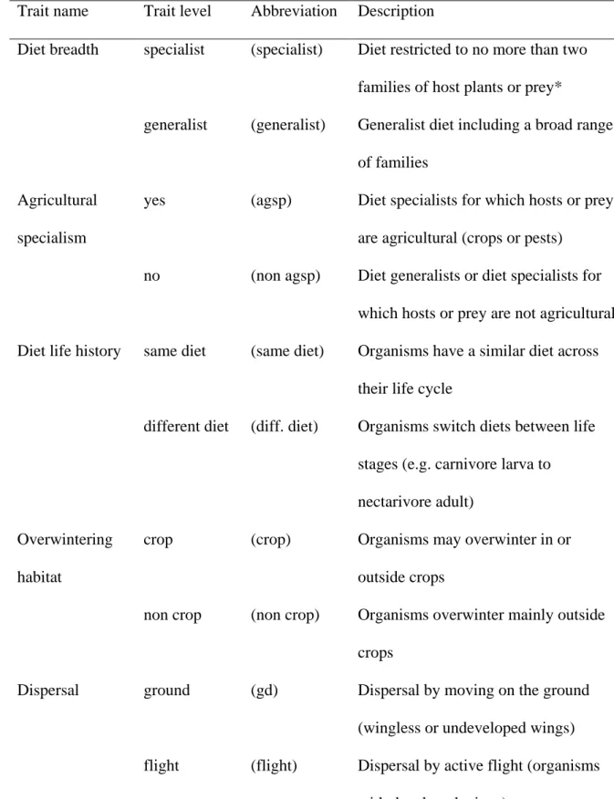
Six categorical traits associated with dispersal mode, overwintering behavior and diet were 303
hypothesized to influence the response of arthropods to landscape variables, as they relate to 304
the need and/or ability to move or disperse between habitat types to access food, hosts, 305
nesting or overwintering resources (Table 1). We defined traits for all arthropod species or 306
families according to the availability of information on separate taxa and to dataset resolution 307
(Appendix S1, Table S2; 36 out of 58 datasets provided species-level identification). We used 308
hierarchical cluster regression to identify parsimonious combinations of shared traits for 309
organisms with shared responses to landscape filters (Appendix S1; Kleyer et al. 2012). These 310
combinations are defined as trait syndromes characterizing different responses of species 311
groups to the environment (see Introduction). As trait syndromes may vary according to the 312
functional group (Lavorel & Garnier 2002), we identified them separately for pollinators, 313
natural enemies and pests (Figs. S3, S4). Trait syndromes are defined parsimoniously based 314
13 on one or a few trait combinations. However, all traits contribute to whole syndrome
315
definition and are described in Figs. S3, S4.
316
Statistical analyses 317
We calculated arthropod abundance in each site at three nested levels of community structure 318
(all arthropods; pollinators, enemies and pests; trait syndromes within functional groups;
319
Appendix S1). Pest control, pollination and yields were available from a subset of studies 320
(Table S3). For this subset, we calculated an ecosystem service index representing the amount 321
of service provided (Appendix S1). We analyzed effects of landscape predictors on arthropod 322
abundance and services using linear mixed effects models in R package lme4 v.1.1-15 (Bates 323
et al. 2015). We focused on abundance because it has been found to drive ecosystem service 324
provision (Winfree et al. 2015). However, abundance and species richness were positively 325
related across groups (estimates of linear mixed models relating richness to abundance using 326
ln(x+1)-transformed data, with random intercept for study and year: 0.4±0.01, p<0.001 for all 327
arthropods, pollinators and enemies). We ln(x+1)-transformed abundance and services to 328
meet assumptions of normality and homoscedasticity. Predictors were % SNH and % arable 329
land as measures of landscape composition, and edge density as measure of configuration. We 330
expected changes at low values of predictors to have more impact than at high values, thus we 331
ln(x+1)-transformed the predictors. This transformation improved model fits (R2, see below) 332
and was maintained for all analyses.
333
To account for collinearity of composition variables (Fig. S2), we performed two sets of 334
models including either % SNH or % arable. Correlations between edge density and 335
composition variables were low within and across studies (Fig. S2; mean within-study 336
Spearman rho 0.05, SD 0.2, mean variance inflation factor of models with all arthropods 2.7, 337
SD 1.8), but some studies showed high correlation in specific years and scales (Table S4). We 338
14 thus ran analyses including and excluding these studies. As no differences were found in 339
overall results, we present analyses including all studies (Appendix S1).
340
Full models took into account hypotheses of a) interactions between landscape variables, and 341
b) non-linearity by including quadratic model terms (Appendix S1). To reflect the ranges 342
covered by European landscape gradients, we did not standardize landscape predictors within 343
studies. In this way we were able to capture non-linear effects across full gradients, i.e. that 344
responses to landscape change within studies may differ across full European gradients in 345
landscape composition and configuration (Van de Pol & Wright 2009). For comparison, we 346
evaluate effects using i) landscape variables mean-centered within studies and ii) standardized 347
response variables in Appendix S3.
348
We accounted for the data’s hierarchical structure by including random effects for study and 349
year, sampling method and block (Appendix S1), and scaled predictors across studies by 350
mean-centering and dividing them by two standard deviations (R package arm v.1.9-3, 351
Gelman & Su 2016). We ran separate models at successive scales of 0.1, 0.25, 0.5, 1, 2 and 3 352
km radius around fields. Results at all scales (estimates and boot-strapped 95% confidence 353
intervals [CI] of full models) are presented Figs. S5-7. Figs. 2-4 illustrate results at 1 km 354
radius. We calculated R2 of the models as the variance explained by fixed (marginal R2, R2m), 355
and by fixed and random terms (conditional R2, R2c), respectively (Nakagawa & Schielzeth 356
2013). Successive spatial scales are inherently correlated, and results at one scale are likely to 357
be reflected at other scales (Martin et al. 2016). In results, we focus interpretation on effects 358
that were significant (CI do not overlap zero) at more than one scale, as these indicate 359
robustness across scales and have the broadest implications for landscape management 360
(Pascual-Hortal & Saura 2007).
361
15 Few studies sampled all taxa and services in the same sites. To avoid lack of common support 362
for contrasts (e.g. a functional group sampled only in a portion of the overall gradient;
363
Hainmueller et al. 2018), we performed separate models for each functional group and 364
service. Replicate numbers for all responses and sites are provided in Tables S5, S6. Residual 365
normality and homoscedasticity were validated graphically. We verified the absence of 366
residual spatial autocorrelation using spline correlograms across studies (Zuur et al. 2009).
367
Statistical analyses were performed in R Statistical Software v. 3.4.1 (R Core Team 2017).
368 369
RESULTS 370
Abundance of arthropods and functional groups 371
We synthesized effects of landscape predictors on the abundance of 132 arthropod families, 372
encompassing over 494,120 individuals and 1,711 identified species or morphospecies. Of 373
these individuals, 50%, 10% and 37% were classified as natural enemies, pollinators and 374
pests, respectively (44%, 33% and 1% of species; Table S2). Effects of % SNH on arthropod 375
abundance were convex at high edge density (Figs. 2, S5). Effects of edge density depended 376
on % SNH, and led to a 2-fold increase at high (>20%) and 1.6-fold increase at low (<2%) 377
SNH. However, in landscapes with low edge density, increasing % SNH had no effect on 378
arthropod abundance.
379
Pollinators, natural enemies and pests showed distinct patterns when considered separately 380
(Fig. 2). Pollinators showed a similar convex effect of % SNH and a negative effect of % 381
arable land (Fig. S5), but effects were scarce on all natural enemies or all pests. The 382
conditional R2 of these models was high (mean maximal R2c across scales 0.80, SD 0.06), but 383
the variance explained by landscape predictors was low (mean maximal R2m across scales 384
16 0.04, SD 0.03). However, breaking up these groups into trait syndromes led to further
385
differentiation and a clearer picture.
386
Trait syndromes of enemies, pollinators and pests 387
Trait syndromes obtained by cluster regression varied between enemies, pollinators and pests, 388
with the most clusters identified among natural enemies (Figs. S3-4). Though scarce overall, 389
effects of landscape predictors on enemies were significant across scales and highly 390
contrasted between trait syndromes (Fig. 3a, S6). Three main patterns emerged: 1) Enemies 391
overwintering outside crops, including flight and ground-dispersers (327 species, 44% of 392
enemies), benefited from high edge density. This was especially true in landscapes with <10%
393
SNH for flyers, and <60% arable land for ground-dispersers (Fig. 3a, S6). These groups 394
increased with increasing % SNH and decreasing % arable land, but effects depended on edge 395
density: they occurred at low (flight) or high edge density (ground-dispersers). 2) In contrast, 396
enemies able to overwinter in crops were most abundant in landscapes with few edges (Fig.
397
3a, S6). Among these, ground-dispersers benefited from high % arable land, but flyers 398
benefited from high % SNH. 3) Effects of landscape predictors on wind-dispersers, mainly 399
ballooning spiders and parasitoid wasps (flight/wind), were scarce.
400
Different responses also emerged among pollinators. Similarly to all arthropods, non- 401
agricultural specialist pollinators increased with high edge density at high or low % SNH 402
(Fig. 3b, S6; 393 species, 70% of pollinators). In contrast, agricultural specialists (e.g.
403
aphidophagous syrphids) were most abundant in landscapes with few edges and high % arable 404
land.
405
Pests able to overwinter in crops showed few effects of landscape variables across scales. But 406
pests considered to leave crops over winter were six times less abundant in landscapes with 407
high edge density (0.2-0.4 km/ha), regardless of their composition (Fig 3c, S6). Due to an 408
17 increase beyond this range at intermediate % SNH, 0.2-0.4 km/ha of edges represented an 409
area of minimum pest density along the observed gradients.
410
Marginal R2 of models including trait syndromes averaged 0.11, SD 0.07 (mean maximal R2m 411
across scales). Thereby, landscape predictors had significantly higher explanatory power 412
when applied to trait syndromes within functional groups, than to whole groups of natural 413
enemies, pollinators and pests (Wilcoxon rank sum test, W=1289, p<0.001).
414
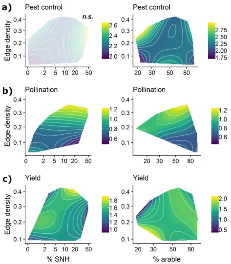
Pest control, pollination and yields 415
Pest control, pollination and yields are given for a subset of studies (Tables S3, S6; Figs. 4, 416
S7). Pest control by natural enemies was highest in landscapes with low % arable land 417
(<40%) and high edge density, where it increased 1.4-fold compared to landscapes with low 418
edge density. It was lowest in coarse-grained landscapes (low edge density) with either low or 419
high % arable land (Fig. 4a). Pollination increased with edge density: it was 1.7 times higher 420
in fine-grained compared to coarse-grained landscapes regardless of % SNH or % arable land.
421
Low pollination was observed in landscapes with >70% arable land and at edge densities <0.1 422
km/ha (Fig. 4b right panel). Yields showed a variable pattern (Fig. 4c, S7). They were highest 423
in landscapes with 10-20% SNH at high edge density (Fig. 4c left panel). Lowest yields were 424
achieved in landscapes with <40% arable land and high edge density (Fig. 4c right panel). In a 425
range of landscapes including a large range of edge density and % arable land, intermediate to 426
high yields were maintained. The variance explained by landscape predictors in models of 427
pest control, pollination and yields averaged 0.14, SD 0.08 (mean maximal R2m across scales;
428
mean maximal R2c 0.60, SD 0. 09).
429
Additional analyses show that effects occurred mainly across full gradients instead of within 430
standardized landscape ranges and were robust to standardization of response variables 431
(Appendix S3), as well as to the analytical method chosen (Appendix S4).
432
18 433
DISCUSSION 434
This synthesis shows that the response of arthropod abundance and services to landscape 435
predictors is non-linear across Europe and depends on interactions between landscape 436
composition and configuration, and on the response traits of arthropods. Overall, arthropods 437
were most abundant in landscapes that combine high edge density with high proportions of 438
semi-natural habitat. Functional groups of pollinators, enemies and pests did not strongly 439
reflect this pattern. Rather, trait syndromes within groups showed contrasting trends.
440
Pollinators that do not feed on pests or crops as larvae (non-pest butterflies, non- 441
aphidophagous syrphids, bees), and flying and ground-dwelling enemies considered to 442
overwinter mainly outside crops, benefited from high edge density at low or high habitat 443
amount and may require a high density of ecotones as exchange interfaces in order to 444
spillover between and into crops (Concepción et al. 2012; Tscharntke et al. 2012; Hass et al.
445
2018). For organisms with limited dispersal ability, this requirement is likely due to the need 446
to recolonize crops in spring. However, the same driver affected strong aerial dispersers such 447
as wasps and butterflies, for which it may be more related to a high sensitivity to disturbance 448
within fields, and/or to the need for resource complementation through a high diversity of 449
available plants and prey (Sutter et al. 2017) or nesting sites. Such diverse resources can be 450
found in neighboring semi-natural habitats (e.g. nest sites; Holland et al. 2016), but also in 451
adjoining crops (pollen and nectar from crops and weeds, host plants or prey for herbivores 452
and predators). Indeed, a high number of separate field units is the first requirement to support 453
a high diversity of arable crops at organism-relevant scales. Landscapes with high vs. low 454
edge density may also differ in their crop composition and/or diversity, with associated 455
impacts on the arthropod community.
456
19 In contrast, ground-dispersing enemies with generalist overwintering needs, and pollinators 457
whose larvae feed on crops or pests, were most abundant in landscapes with few edges and 458
high % arable land. These groups benefit from agricultural resources and were able to 459
maintain populations in coarse-grained landscapes with high % arable land that other 460
organisms avoided. They thus represent important insurance organisms contributing to 461
arthropod response diversity (Cariveau et al. 2013), and may continue to provide services in 462
coarse-grained landscapes with little non-crop habitat (Rader et al. 2016; but see Stavert et al.
463
2017). However, abundances were too low for these trends to be reflected in overall patterns.
464
In addition, pests also benefited from landscapes with low edge density. The services 465
provided by agriculture-resilient enemies and pollinators are thus likely insufficient to balance 466
the bottom-up effects of high crop resource availability on pests in such low complexity 467
landscapes (Walker & Jones 2003).
468
Pests overwintering outside crops were least abundant, and pollination and pest control were 469
highest, in landscapes with high edge density, particularly within the range of 0.2-0.4 km/ha.
470
In agreement with Rusch et al. (2016), pest control was also highest at low % arable land. But 471
for pests and pollination, edge density effects occurred largely independently of landscape 472
composition. Based on trait syndrome patterns, pest control and pollination appear to have 473
been largely driven by organisms without strong links to agricultural resources, which 474
benefitted from high edge density to spillover and provide services in crops (ground- and to a 475
lesser extent flight-dispersing enemies overwintering outside crops for pest control; non- 476
agricultural specialists for pollination). Due to positive impacts on services and many service 477
providers and negative impacts on pests, edge density thus appeared a more consistent driver 478
for functional biodiversity and service provision than the presence of semi-natural habitat 479
alone (Concepción et al. 2012). High diversity of arthropod service providers in such 480
landscapes, confirmed by a positive correlation between abundance and species richness, may 481
20 further imply functional redundancy. As a result, services supported by these landscapes may 482
be more resilient to environmental change (Oliver et al. 2015, Martin et al. in press).
483
Landscapes with high edge density did not have lower yields/area than coarse-grained 484
landscapes, in a large portion of composition gradients with varying % SNH and arable land.
485
Though only available from a subset of the data (Table S6), this result indicates that high edge 486
density and its benefits can be combined with maintaining crop yields, within the range of 487
edge density observed here. Accordingly, productive landscapes with edge density between 488
0.2 and 0.4 km/ha may be ideally suited to implement ecological intensification. Cascading 489
(positive) effects on yields of higher service provision and less pests in landscapes with high 490
edge density were not, however, apparent from the available data. Reduced pollination and 491
pest control at low edge density may have been compensated by external inputs in productive 492
landscapes. In addition, other factors combine to impact yields (Gagic et al. 2017) and may 493
mask the impact of biodiversity-driven services in the absence of careful standardization 494
(Pywell et al. 2015). Intermediate to low yields in landscapes with high % arable, low % SNH 495
and low edge density may underpin the risks of ongoing conventional intensification resulting 496
in yield stagnation or reduction despite high agricultural inputs (Ray et al. 2012).
497
Non-linear and interacting effects of landscape predictors denote the importance of variation 498
in the ranges occupied by European landscape gradients between studies. In combination with 499
trait-based response syndromes, these results explain several inconsistencies highlighted in 500
previous work (Kennedy et al. 2013; Veres et al. 2013; Díaz & Concepción 2016; Holzschuh 501
et al. 2016; Rader et al. 2016; Tscharntke et al. 2016; Karp et al. 2018). By covering a wide 502
range of landscapes and responses, this study helps resolve why responses to landscape 503
configuration and composition of arthropod functional groups differ along landscape 504
gradients. In particular, we show that landscape effects and the potential effectiveness of 505
landscape management measures vary according to the ranges of landscape variables captured 506
21 in each study region, in agreement with theory underlying non-linear responses of organisms 507
to landscape gradients (Concepción et al. 2012). Increasing edge density was most effective 508
for arthropods in landscapes with low (<5%) or high (>20%) % SNH. In landscapes with 509
intermediate % SNH, small increases in SNH may dilute populations, evening out the benefits 510
of many edges, before reaching sufficient levels to contribute positively to spillover into 511
fields. In these landscapes, extensive practices such as low-input farming may be the most 512
effective way to enhance arthropod diversity and services in crops (Jonsson et al. 2015).
513
Contrary to our hypotheses (Fig. 1), few effects were hump-shaped within the range of tested 514
gradients, thus maxima may not be reached within the measured European gradients.
515
We applied a trait-based framework for agroecosystem communities using response traits that 516
have not been considered in previous work on pollinators (Williams et al. 2010; De Palma et 517
al. 2015; Carrié et al. 2017) or grassland arthropods (Gámez-Virués et al. 2015), but were 518
important determinants of species’ responses to landscape structure. We found that syndromes 519
combining several response traits effectively disentangled pollinator, pest and enemy 520
responses compared to single-trait approaches. Considering such traits with strong 521
mechanistic underpinnings (Bartomeus et al. 2018) will increase our ability to derive 522
predictions of the effects of environmental change on communities. Clarification is needed, 523
however, on which trait syndromes correlate with strong impacts on service provision in 524
crops. For instance, non-bees may complement bees for provision of pollination services 525
(Rader et al. 2016), but the separate contribution of non-bee pollinators in intensive 526
landscapes is unknown, and according to our results, may be considerably lower. In addition, 527
relative contributions to pest control of natural enemies with different landscape responses, 528
and the importance of high enemy diversity for pest control in real-world landscapes, have yet 529
to be elucidated.
530
Conclusion 531
22 In this synthesis across Europe, we show that within European gradients, a high edge density 532
is beneficial for a wide range of arthropods and the services they provide, and can be 533
combined with high yields in productive landscapes with over 50% arable land. In addition to 534
managing semi-natural habitat amounts, increasing the edge density of these landscapes is a 535
promising pathway to combine the maintenance of arthropod biodiversity and services with 536
continued and sustainable agricultural production. While the strength of these effects for 537
arthropods depends on habitat amount, fine-grained landscapes provided benefits such as less 538
pests and more pollination, which were largely independent of their composition. We further 539
demonstrate a high response diversity of arthropod service providers leading to differing 540
impacts of landscape change within groups of natural enemies, pests and pollinators. We thus 541
call for consideration of mechanism-relevant response traits to catalyze modelling and 542
prediction of the consequences of land-use change on arthropods and ecosystem services in 543
crops.
544 545
ACKNOWLEDGEMENTS 546
We thank all farmers, field and technical assistants, researchers and funders who contributed 547
to the studies made available for this synthesis. F. Bötzl and L. Pfiffner provided expertise 548
and data on carabid traits. M. O’Rourke provided expertise on pest traits. A. Kappes, S. König 549
and D. Senapathi provided technical support. We thank all members of the Socio- 550
Environmental Synthesis Center working group on ‘Decision-making tools for pest control’
551
led by D. Karp and B. Chaplin-Kramer for fruitful discussions in the process of creating this 552
paper. We are grateful to three anonymous reviewers and to the editor for constructive 553
comments on a previous version of the manuscript. Funding was provided by the European 554
Union to the FP7 project LIBERATION (grant 311781) and by the 2013–2014 555
23 BiodivERsA/FACCE-JPI joint call for research proposals (project ECODEAL), with the 556
national funders ANR, BMBF, FORMAS, FWF, MINECO, NWO and PT-DLR. E.D.C., 557
M.Díaz, and G.M. acknowledge the project BIOGEA (PCIN-2016-159, BiodivERsA3 with 558
the national funders BMBF, MINECO, BNSF).
559 560
REFERENCES 561
Bates, D., Mächler, M., Bolker, B. & Walker, S. (2015). Fitting linear mixed-effects models 562
using lme4. J. Stat. Softw., 67.
563
Bartomeus, I., Cariveau, D.P., Harrison, T. & Winfree, R. (2018). On the inconsistency of 564
pollinator species traits for predicting either response to land-use change or functional 565
contribution. Oikos, 127, 306–315.
566
Blitzer, E.J., Dormann, C.F., Holzschuh, A., Klein, A.-M., Rand, T.A. & Tscharntke, T.
567
(2012). Spillover of functionally important organisms between managed and natural 568
habitats. Agric. Ecosyst. Environ., 146, 34–43.
569
Boetzl, F.A., Krimmer, E., Krauss, J., Steffan‐Dewenter, I. (2019). Agri‐environmental 570
schemes promote ground‐dwelling predators in adjacent oilseed rape fields: Diversity, 571
species traits and distance‐decay functions. J. Appl. Ecol., 56, 10–20.
572
Bommarco, R., Kleijn, D. & Potts, S.G. (2013). Ecological intensification: harnessing 573
ecosystem services for food security. Trends Ecol. Evol., 28, 230–238.
574
Bosem Baillod, A., Tscharntke, T., Clough, Y. & Batáry, P. (2017). Landscape-scale 575
interactions of spatial and temporal cropland heterogeneity drive biological control of 576
cereal aphids. J. Appl. Ecol., 54, 1804–1813.
577
Brown, A.M., Warton, D.I., Andrew, N.R., Binns, M., Cassis, G. & Gibb, H. (2014). The 578
fourth-corner solution–using predictive models to understand how species traits 579
interact with the environment. Methods Ecol. Evol., 5, 344–352.
580
Cariveau, D.P., Williams, N.M., Benjamin, F.E. & Winfree, R. (2013). Response diversity to 581
land use occurs but does not consistently stabilise ecosystem services provided by 582
native pollinators. Ecol. Lett., 16, 903–911.
583
Carrié, R., Andrieu, E., Cunningham, S.A., Lentini, P.E., Loreau, M. & Ouin, A. (2017).
584
Relationships among ecological traits of wild bee communities along gradients of 585
habitat amount and fragmentation. Ecography, 40, 85–97.
586
Chaplin-Kramer, R., O’Rourke, M.E., Blitzer, E.J. & Kremen, C. (2011). A meta-analysis of 587
crop pest and natural enemy response to landscape complexity. Ecol. Lett., 14, 922–
588
932.
589
Concepción, E.D., Díaz, M., Kleijn, D., Báldi, A., Batáry, P., Clough, Y., et al. (2012).
590
Interactive effects of landscape context constrain the effectiveness of local agri- 591
environmental management. J. Appl. Ecol., 49, 695–705.
592
Coudrain, V., Schüepp, C., Herzog, F., Albrecht, M. & Entling, M.H. (2014). Habitat amount 593
modulates the effect of patch isolation on host-parasitoid interactions. Front. Environ.
594
Sci., 2.
595
24 De Palma, A., Kuhlmann, M., Roberts, S.P.M., Potts, S.G., Börger, L., Hudson, L.N., et al.
596
(2015). Ecological traits affect the sensitivity of bees to land-use pressures in 597
European agricultural landscapes. J. Appl. Ecol., 52, 1567–1577.
598
Díaz, M. & Concepción, E.D. (2016). Enhancing the effectiveness of CAP greening as a 599
conservation tool: A plea for regional targeting considering landscape constraints.
600
Curr. Landsc. Ecol. Rep., 1, 168–177.
601
Duflot, R., Aviron, S., Ernoult, A., Fahrig, L. & Burel, F. (2015). Reconsidering the role of 602
‘semi-natural habitat’ in agricultural landscape biodiversity: a case study. Ecol. Res., 603
30, 75–83.
604
Dunning, J.B., Danielson, B.J. & Pulliam, H.R. (1992). Ecological processes that affect 605
populations in complex landscapes. Oikos, 169–175.
606
Fahrig, L. (2013). Rethinking patch size and isolation effects: the habitat amount hypothesis.
607
J. Biogeogr., 40, 1649–1663.
608
Fahrig, L. (2017). Ecological responses to habitat fragmentation per se. Annu. Rev. Ecol.
609
Evol. Syst., 48.
610
Fahrig, L., Girard, J., Duro, D., Pasher, J., Smith, A., Javorek, S., et al. (2015). Farmlands 611
with smaller crop fields have higher within-field biodiversity. Agric. Ecosyst.
612
Environ., 200, 219–234.
613
Foley, J.A., DeFries, R., Asner, G.P., Barford, C., Bonan, G., Carpenter, S.R., et al. (2005).
614
Global Consequences of Land Use. Science, 309, 570–574.
615
Gagic, V., Kleijn, D., Báldi, A., Boros, G., Jørgensen, H.B., Elek, Z., et al. (2017). Combined 616
effects of agrochemicals and ecosystem services on crop yield across Europe. Ecol.
617
Lett., 20, 1427–1436.
618 Gámez-Virués, S., Perović, D.J., Gossner, M.M., Börschig, C., Blüthgen, N., Jong, H. de, et 619
al. (2015). Landscape simplification filters species traits and drives biotic 620
homogenization. Nat. Commun., 6, 8568.
621
Garnett, T., Appleby, M.C., Balmford, A., Bateman, I.J., Benton, T.G., Bloomer, P., et al.
622
(2013). Sustainable Intensification in Agriculture: Premises and Policies. Science, 341, 623
33–34.
624
Geiger, F., Bengtsson, J., Berendse, F., Weisser, W.W., Emmerson, M., Morales, M.B., et al.
625
(2010). Persistent negative effects of pesticides on biodiversity and biological control 626
potential on European farmland. Basic Appl. Ecol., 11, 97–105.
627
Gelman, A. & Su, Y.-S. (2016). arm: Data Analysis Using Regression and 628
Multilevel/Hierarchical Models. R package version 1.9-3. https://CRAN.R- 629
project.org/package=arm.
630
Haddad, N.M., Gonzalez, A., Brudvig, L.A., Burt, M.A., Levey, D.J. & Damschen, E.I.
631
(2017). Experimental evidence does not support the Habitat Amount Hypothesis.
632
Ecography, 40, 48–55.
633
Hainmueller, J., Mummolo, J. & Xu, Y. (2018). How Much Should We Trust Estimates from 634
Multiplicative Interaction Models? Simple Tools to Improve Empirical Practice 635
(SSRN Scholarly Paper No. ID 2739221). Social Science Research Network, 636
Rochester, NY.
637
Hass, A.L., Kormann, U.G., Tscharntke, T., Clough, Y., Baillod, A.B., Sirami, C., et al.
638
(2018). Landscape configurational heterogeneity by small-scale agriculture, not crop 639
diversity, maintains pollinators and plant reproduction in western Europe. Proc R Soc 640
B, 285, 20172242.
641
Holland, J.M., Bianchi, F.J., Entling, M.H., Moonen, A.-C., Smith, B.M. & Jeanneret, P.
642
(2016). Structure, function and management of semi-natural habitats for conservation 643
biological control: a review of European studies. Pest Manag. Sci., 72, 1638–1651.
644


![adistincttypeofenergyproductionsystem,nowadaysmainlyrenewableenergy.Similartoother energysourcescanbefoundinmanycountries,fromtheUSAtoChinaandacrossEurope[ – ]. energylandscape;Eurasianskylark;landcover;landuse;land-coverheterogeneity; withtheareaoftheinl](data:image/gif;base64,R0lGODlhAQABAIAAAP///wAAACH5BAEAAAAALAAAAAABAAEAAAICRAEAOw==)