Global Ecology and Conservation 28 (2021) e01663
Available online 4 June 2021
2351-9894/© 2021 The Author(s). Published by Elsevier B.V. This is an open access article under the CC BY license
Roads reduce amphibian abundance in ponds across a fragmented landscape
Andrew J. Hamer
a,b,*,1, Barbara Barta
b,c,2, Attila Bohus
b,d,3, Blanka G ´ al
b,4, D ´ enes Schmera
b,5aCentre for Ecological Research, GINOP Sustainable Ecosystems Group, Klebelsberg K. u. 3, H-8237 Tihany, Hungary
bBalaton Limnological Research Institute, E¨otv¨os Lor´and Research Network (ELKH), Klebelsberg K. u. 3, H-8237 Tihany, Hungary
cInstitute of Aquatic Ecology, Centre for Ecological Research, Karolina út 29, 1113 Budapest, Hungary
dResearch Group of Limnology, Center for Natural Sciences, University of Pannonia, Egyetem u. 10, H-8200 Veszpr´em, Hungary
A R T I C L E I N F O Keywords:
Accessible habitat Animal abundance Community ecology N-mixture model Road ecology Wetlands
A B S T R A C T
Roads threaten animal species through habitat loss, fragmentation and degradation, and direct mortality. It is crucial to understand how species respond to linear infrastructure for effective conservation of animal communities in fragmented landscapes. We assessed relationships be- tween amphibian abundance and roads/ railways and habitat fragmentation. We examined whether the combined effects of habitat loss and roads or railways (accessible habitat) was a better predictor of amphibian abundance than (1) the total amount of habitat surrounding ponds, (2) distance to a highway or railway, or (3) surrounding road cover. Aquatic surveys for amphibian larvae were conducted at 30 freshwater ponds over the breeding season in a mixed peri-urban/ agricultural landscape in Hungary. Landscape variables were quantified within a 1000-m radius surrounding ponds and habitat variables were measured at the local (pond) scale.
The larvae of seven amphibian species were detected. There were strong relationships between the abundance of amphibian larvae and the distance to a highway and the proportion of road cover within 1000 m of ponds. Relationships with accessible habitat and total habitat amount were uncertain, while there were no clear relationships with a major railway. Larval abundance increased with pond size, but there were mixed relationships with the presence of fish. Our results suggest that road effects were having a stronger impact on amphibian abundance than the combined effects of roads and habitat amount in the study area. Highways appeared to be negatively impacting amphibian communities within a wide road-effect zone up to 1 km from ponds. However, our results were obtained from a single-season snap-shot study and multi-season surveys are likely required to reduce uncertainty in the model predictions. Our analysis suggests that road mitigation projects for amphibians should create large ponds in areas with no highways and low road density, and with connectivity to surrounding habitats.
* Corresponding author at: Centre for Ecological Research, GINOP Sustainable Ecosystems Group, Klebelsberg K. u. 3, H-8237 Tihany, Hungary.
E-mail address: a.hamer@unimelb.edu.au (A.J. Hamer).
1 https://orcid.org/0000-0001-6031-7841.
2 https://orcid.org/0000-0002-6674-3275.
3 https://orcid.org/0000-0001-5733-8633.
4 https://orcid.org/0000-0001-8513-3010.
5 https://orcid.org/0000-0003-1248-8413.
Contents lists available at ScienceDirect
Global Ecology and Conservation
journal homepage: www.elsevier.com/locate/gecco
https://doi.org/10.1016/j.gecco.2021.e01663
Received 20 January 2021; Received in revised form 2 June 2021; Accepted 2 June 2021
1. Introduction
Urbanisation is regarded as one of the greatest threats to biodiversity and affects many of Earth’s ecosystems through habitat loss, fragmentation and degradation (Czech et al. 2000; Grimm et al. 2008; Shochat et al. 2010). The European continent is highly urbanised and it is predicted that by 2050, 74% of the human population in Europe will live in cities (UNDESA, 2018). This shift in the dis- tribution of the human population will likely have profound impacts on biodiversity in both rural and urban areas, with exponential growth of linear infrastructures continuing to fragment the landscape (Pullin et al. 2009).
Roads are built to service growing cities and towns and are one of the most pervasive forms of urbanisation (van der Ree et al.
2015). At least 25 million kilometres of new roads are anticipated to be built globally by 2050; a 60% increase in the total length of roads over that in 2010 (Laurance et al. 2014). Torres et al. (2016) reported that almost a quarter of all land area in Europe (22.4%) is located within 500 m of the nearest transport infrastructure, and 50% is within 1.5 km, leading to declining populations of birds and mammals. Indeed, Europe is probably the continent most highly fragmented by transport infrastructures (Selva et al. 2011). Central European countries also follow this trend (Selva et al. 2011), and since 2010, 500 km of new highways have been built in Hungary (MTI, 2020). This will likely have severe implications for local and regional biodiversity.
Roads and road traffic impact wildlife in many ways, ranging from direct mortality to alteration of the biophysical environment in a road-effect zone (Forman, 2000; van der Ree et al. 2015). The ecological effects of roads on aquatic and terrestrial habitats are numerous and diverse (Findlay and Bourdages, 2000; Trombulak and Frissell, 2000); e.g. road construction often destroys, fragments and degrades aquatic and terrestrial habitats on which many wetland-dependent species depend (Forman and Alexander, 1998;
Trombulak and Frissell, 2000). Rail infrastructure can also have similar impacts on wildlife, bisecting animal populations and causing mortality (Barrientos et al. 2019). Consequently, roads and railways are endangering many animal species that rely on connectivity between aquatic and terrestrial habitats (Dorsey et al. 2015; Hamer and McDonnell, 2008; Trombulak and Frissell, 2000).
Amphibians are one of the most imperiled animal groups with one-third of species at risk of extinction due to urbanisation (Hamer and McDonnell, 2008). Pond-breeding amphibians depend on inter-connected networks of freshwater ponds to complete their complex life cycles (Semlitsch, 2000), which makes them particularly sensitive to wetland loss, fragmentation and degradation (Cushman, 2006; Hamer and McDonnell, 2008), and vulnerable to impacts from road construction and traffic (Beebee, 2013; Hamer et al. 2015;
Hels and Buchwald, 2001). Furthermore, amphibians are highly vulnerable to road mortality because they are slower and smaller relative to other vertebrate taxa (Rytwinski and Fahrig, 2012). Highly vagile amphibian species are at greater risk of road mortality because they will often encounter roads with greater frequency (Carr and Fahrig, 2001; Gibbs, 1998). Dispersal barriers between aquatic breeding habitats and terrestrial habitat areas may impair metapopulation dynamics and lead to a reduction in the size of regional populations (Becker et al. 2007; Semlitsch, 2002). There is generally a decrease in the occurrence and abundance of amphibian species in fragmented landscapes supporting high traffic volumes (Cayuela et al. 2015; Hartel et al. 2010), often because forest cover is negatively correlated with the density of roads and traffic (Eigenbrod et al. 2008a).
Amphibian declines in central European countries such as Hungary have been attributed to the construction of roads which, along with other forms of landscape change, have destroyed 97% of wetlands (V¨or¨os et al. 2015). Road construction in Hungary since 2004 has led to net habitat loss, degradation and decline in biodiversity (Mih´ok et al. 2017). The construction of roads in many areas has disconnected amphibian populations and created barriers between their hibernation and breeding sites (V¨or¨os et al. 2015). As such, there is a call for more basic research in Hungary to understand the effects of roads on amphibians, and to develop effective long-term conservation programmes (Vor¨¨os et al. 2015). This research would also fill a gap in our knowledge of how amphibians respond to linear infrastructure in central and eastern Europe at landscape scales.
Accessible habitat has been used to quantify the effects of roads on amphibian populations separately from habitat loss (Eigenbrod et al. 2008b; Hamer, 2016; Hamer, 2018). It is defined as the amount of terrestrial habitat (e.g. forest patch) that can be reached from a focal patch of habitat (e.g. breeding pond) without crossing a road or railway (Eigenbrod et al. 2008b). Unfragmented habitats are more likely to contribute to community richness and abundance than habitat on the other side of the road because critical life-history processes (e.g. dispersal between hibernation and breeding sites) can be maintained. Additionally, a major road (e.g. 4-lane highway) that needs to be crossed to access other habitat patches is likely to have a much greater negative effect on the population than a smaller road that does not restrict access to habitat (e.g. 2-lane secondary road). There are also likely to be differences between roads and railways in their relative contribution to habitat fragmentation (Selva et al. 2011), but this effect has not been tested empirically. An increasing proportion of accessible habitat (e.g. forest cover) within barrier-based buffers extending up to 2500 m around ponds has been shown to increase anuran occupancy in western Europe (Zanini et al. 2008), and sealed roads and urban cover surrounding ponds in eastern European landscapes also decrease amphibian occupancy and abundance (Hartel et al. 2009a; Hartel et al. 2010). However, no studies have applied the concept of accessible habitat to assess the relative effects of roads and railways in fragmenting landscapes occupied by amphibian communities in central or eastern Europe.
We conducted a study into the relationships between road and rail infrastructure and the abundance of larval amphibian com- munities in a highly-fragmented landscape in central Europe. We focussed on abundance within the larval stages because of the strong correlation between habitat quality and species demography (Van Horne, 1983), although we acknowledge that understanding
juvenile demography may be more critical for determining the effects of roads on amphibian populations (Petrovan and Schmidt, 2019). There is also likely to be wide variability in the size of larval populations from year to year due to a range of factors (e.g.
hydroperiod), leading to variable juvenile recruitment that can affect community structure (Semlitsch et al. 1996). Accordingly, our study provided a snap-shot of the abundance of larval communities over one breeding season. We assumed that ponds with high larval abundance would have potentially higher numbers of metamorphosing juveniles, provided they did not dry out. We predicted that accessible habitat is a better predictor of larval amphibian abundance than (1) the total amount of habitat surrounding ponds, (2) distance to a highway, or (3) road cover surrounding ponds, based on previous investigations which found that accessible habitat was a better predictor of amphibian species richness and occupancy (Eigenbrod et al. 2008b; Hamer, 2016). We also determined whether using a main railway line to calculate accessible habitat was a better predictor of amphibian abundance than using highways, and we determined the relative influence of local habitat variables on amphibian abundance. In the latter, we predicted that: (1) amphibian abundance will increase with increased pond area, and (2) amphibian abundance will decrease with fish presence in ponds. We assessed local habitat variables because amphibian breeding distribution in fragmented landscapes is often influenced by multiple factors at both the local and landscape scales that can affect population size (Hamer and Parris, 2011; Rubbo and Kiesecker, 2005; Van Buskirk, 2005). For instance, fish have the potential to eliminate entire cohorts of amphibian larvae through predation (Kats and Ferrer, 2003). We discuss the implications of our results for conserving amphibians in areas bisected by roads and other linear infrastructure.
2. Methods 2.1. Study area
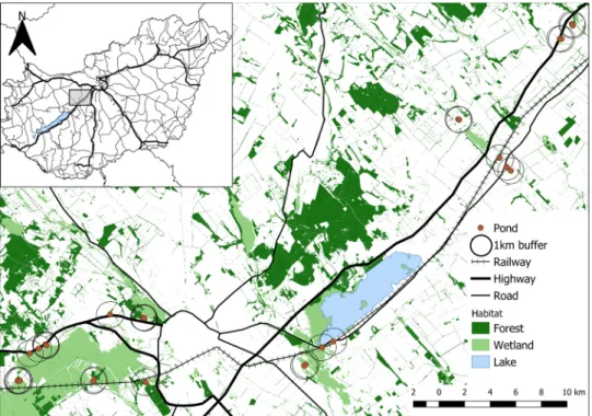
The study area was approximately 50 km south-west of Budapest, Hungary, comprised predominantly of agricultural land but also included small towns, floodplains and nature conservation areas (Fig. 1); therefore, it was a mixed peri-urban/ agricultural landscape.
The study area contained several highways (M7 motorway, no. 7, no. 8 and no. 801 roads, all ≥4-lanes) and the main railway line from Budapest to Veszpr´em. Hence, the study area covered a broad landscape highly fragmented by transportation infrastructure, which was an ideal system to examine the response of amphibian communities to roads and railways.
We initially selected up to 50 ponds (lentic waterbodies) in the study area using Google Earth Pro images (Google Inc., 2020) and the Ecosystem Base Map of Hungary (Ministry of Agriculture, 2019). Constraints on property access and water availability at some sites resulted in a final set of 30 ponds being selected. Site selection ensured there was sufficient variation in pond area, distance to highways and the extent of natural and urban features in the surrounding landscape. Site types included highway stormwater retention ponds, recreational fishing ponds, farm dams, ditches and canals, and floodplain ponds. Sites were grouped into 12 spatial clusters
Fig. 1.Map of the study area in western Hungary. Highways =sealed roads, ≥4 lanes; Roads =sealed roads, 2 lanes. Habitat classed as "Lake" was included under wetland habitat in the analysis.
comprised of 1 – 5 sites, with sites in the same cluster being <1000 m apart, to approximate the mean dispersal distances of adult amphibians expected to occur in the study area (Smith and Green, 2005). Sites within clusters were typically separated by vegetated areas (e.g. grassland) with no intervening urban infrastructure, highways, the main railway or other obvious barriers. Mean distance to the nearest surveyed site was 411 m (SD=838; range: 14 – 3977 m).
2.2. Larval amphibian surveys
Three aquatic surveys were conducted at the 30 ponds over one breeding season in spring and summer (survey 1: April/May 2020;
survey 2: June 2020; survey 3: July 2020), corresponding with the breeding season of amphibian species recorded in the region (Berninghausen and Berninghausen, 2001). Repeated surveys were undertaken to reduce uncertainties that may arise from high variability in larval abundance within a single season. Sites were surveyed during the day by dip-netting at ponds with sufficient water levels (water depth >5 cm) using a net specifically designed for the safe capture of amphibians (300-mm wide frame, 350 mm deep, 1 mm mesh size). The number of net sweeps was scaled in proportion to pond area – one net sweep for every 25 m2 of pond surface area (Shulse et al. 2010), with 2 – 281 sweeps per pond (mean=45, SD=56). The number of net sweeps was modified at sites with reduced water levels, but still scaled in proportion to the inundated area. Dip-net sweeps were approximately 1.5 m in length and were per- formed in all microhabitat types (e.g. open water, emergent/ submerged vegetation) to target the microhabitat preferences of amphibian larvae (Shaffer et al. 1994). Water temperature was recorded at the shoreline. Ponds within the same spatial cluster were generally surveyed on the same day and survey timing of each cluster was randomised to minimise bias.
In small ponds (<1000 m2) and some larger ponds, amphibian larvae caught in dip-nets were held temporarily in a plastic bucket and then identified, counted and released unmarked. In large ponds, amphibian larvae were processed upon capture and then released; the distance between the point of release and the next dip-net sweep was >5 m to avoid double-counting individuals. The count of all organisms (e.g. fish) captured in dip-nets was recorded. The presence of fish at sites was also confirmed visually. Amphibian larvae were identified to species using Berninghausen and Berninghausen (2001). Taxonomy follows Speybroeck et al. (2020). Larvae of green frogs (Pelophylax lessonae, P. kl. esculenta and P. ridibunda) were consolidated under the Pelophylax spp. complex. Frog and toad larvae were defined as individuals within Gosner development stages 25 (small tadpoles large enough to be reliably identified) through stages 42–44 (metamorphosing tadpoles with front and hind limbs; Gosner, 1960); newt larvae were identified using similar morphological pa- rameters (stages 39–55; Gallien and Bidaud, 1959). Standard hygiene protocols to minimise the risk of spreading the amphibian chytrid fungal diseases Batrachochytrium dendrobatidis and B. salamandrivorans were followed when conducting fieldwork (Phillott et al. 2010).
Fieldwork was conducted under protocols to minimise the risk of transmitting the human coronavirus (COVID-19).
2.3. Landscape-scale variables
Accessible habitat (%) was defined as the total area of forest and wetland habitat within a 1000-m radius of a pond edge that could be accessed without crossing only highways (Access_hwy) or highways and the main railway (Access_hwy_rail). Forest habitat included forests, woodland and woody/ herbaceous vegetation, whereas wetland habitat included permanent and temporary marshes and lakes.
A 1000-m radius was selected as the landscape buffer to cover the dispersal distances of most amphibian species expected to occur in the study area (Smith and Green, 2005; Vos and Stumpel, 1995), which was smaller than the maximum dispersal distance recorded for some species (Smith and Green, 2005). We assumed that highways represented the greatest barrier to amphibian movement in the study area, and that sealed 2-lane roads with a smaller physical footprint and presumably lower traffic volumes were having a weaker barrier effect (Eigenbrod et al. 2008b). We also predicted that the railway would have a smaller barrier effect than highways for similar reasons. Accordingly, highways and the railway were used to delineate accessible habitat. The total area of forest and wetland habitat within a 1000-m radius of a pond (Habitat%), ignoring the presence of highways and the railway within the buffer, was included as a separate variable to assess habitat area in predicting the effect of habitat loss on amphibian abundance, separately from road effects.
Road cover (%) within a 1000-m radius around a pond (Roads) was calculated using mapped road surfaces and used to assess the effect of the total area (length and width) of all sealed roads on amphibian abundance in the study area, separately from habitat loss. Road cover is also a surrogate variable for the degree of urbanisation around a site as it is often correlated with the density of urban infrastructure (Hamer and McDonnell, 2008; Parris, 2006). The distance from a pond margin to the nearest highway (Dist_hwy) or to a highway or the railway (Dist_hwy_rail) was measured to assess road and rail effects separately, and to determine if a road-effect zone was affecting amphibian abundance in ponds close to highways and the railway. QGIS v.3.10 was used to measure distances and for all area calculations (QGIS Development Team, 2020).
2.4. Local-scale variables
Hydroperiod and the presence of predatory fish species are often important determinants of amphibian community structure (Wellborn et al. 1996). We recorded the presence of fish (Fish) at sites during the aquatic surveys (fish presence =1; non-detection =0) and scored hydroperiod according to the percentage of the full water-holding capacity of each pond during field surveys. Ephemeral ponds (1) were completely dry on at least one survey; semi-permanent ponds (2) dried down to ≤20% of full water levels; permanent ponds (3) retained >20% of full capacity throughout the study. Increased pond area and hydroperiod have been shown to reduce turnover in metacommunities of larval amphibians, while fish presence decreases population densities (Werner et al. 2007). Larger habitat patches can also support higher animal population sizes within metapopulations (Hanski, 1994). Hence, pond area (Area) was included and calculated from digitised polygons using Google Earth Pro.
2.5. Modelling
Multi-species abundance models (MSAM) were developed to assess relationships between the abundance of amphibian larvae at ponds and the landscape- and local-scale variables. A MSAM is a hierarchical (community) N-mixture model that allows abundance to be estimated from repeated count surveys while adjusting for imperfect detection of individuals (Royle, 2004; Royle et al. 2007; Royle et al. 2005). Models for individual species are linked together into a hierarchical model so that collectively they represent community-level responses to environmental covariates, which increases the precision of parameter estimates for species observed at few sites by considering each within the context of the broader community and borrowing strength from more abundant species (Dorazio et al. 2006; K´ery and Royle, 2008; Zipkin et al. 2009). These models therefore account for interspecific variation in egg clutch size and other reproductive parameters by estimating the mean larval abundance across all species in the community and then relating mean community abundance to covariates.
The MSAM were built from a series of individual N-mixture models using the original formulation of Royle (2004) and Royle et al.
(2005), using count data from larval surveys. The first level of the model (sub-model) assumed true but imperfectly observed abun- dance, where the abundance of species i at site j, Nij, is a Poisson random variable:
Nij ~ Poisson(λij)
where λij is the expected (or mean) abundance (Royle et al. 2005). A random effects term for spatial autocorrelation (Cluster) was added to models because breeding dispersal of adult amphibians may be occurring between closely-spaced wetlands (e.g. <100 m apart), resulting in spatially-aggregated patterns of larval abundance in breeding ponds. The spatial aggregation of sites in the study area also resulted in overlapping and therefore non-independent landscape buffers. Failing to account for spatial autocorrelation can lead to biased parameter estimates (Wintle and Bardos, 2006), whereas overlapping landscape buffers can result in lower variation in predictor variables (Eigenbrod et al. 2011); however, there was sufficient variation in the covariates we examined (Appendix A:
Table S1). Overdispersion is a common phenomenon in count data and can bias parameter and abundance estimates in N-mixture models (Knape et al. 2018; Link et al. 2018). A random effects term for overdispersion and unexplained variation in abundance (ε) was therefore included in each model (K´ery et al. 2009). Mean abundance was expressed as a log-linear function of site-level covariates in six separate models:
log(λij) =β0i +β1i (Areaj) +β2i (Xj) +β3i (Fishj) +Clusterj +εi
where Xj is one of six landscape-scale covariates calculated at site j (Access_hwy, Access_hwy_rail, Habitat, Roads, Dist_hwy, Dis- t_hwy_rail). The covariates Dist_hwy, Dist_hwy_rail and Area were log10(x)-transformed prior to analysis. Area was included in all models to account for variation in pond size, and hence, sampling area. Each sub-model had a maximum of three covariates given the recommendation of a minimum n/k of 10 where n is the number of sites and k is the number of estimated parameters (Harrison et al.
2018). Fish was selected for inclusion over Hydroperiod because fish predators can eliminate amphibian larvae from ponds and can colonise ephemeral ponds during floods (Semlitsch, 2002). There was no strong correlation between Hydroperiod and Fish (rs
=0.445), or among the covariates included in each model (|r| or |rs| <0.6; Table S2).
The probability of detection was modelled using the proportion of full water-holding capacity of a site (Water); water temperature (Temp); and the number of days since 1 February 2020 (Days). Reduced water levels at a site may increase larval densities and hence affect detectability; conversely, increased water levels may encourage breeding activity and spawning (Hartel et al. 2011). Higher water temperatures are likely to increase larval activity (Wells, 2007). The covariate Days accounts for variation in detection since the beginning of the breeding season, as species differ in timing of spawning (Berninghausen and Berninghausen, 2001); detection of species with a prolonged reproductive strategy is likely to increase over the season, whereas detection of early breeding species will decrease with Days (Wells, 1977). Detection was modelled as a binomial process:
Cijk ~ Binomial(pijk, Nij)
where Cijk is the number of detected individuals (i.e. count) of species i at site j on survey k, and pijk is the probability of detecting each individual of species i at site j on survey k (Royle et al. 2005). Detection probability was expressed as a logit-link function of the three survey-specific covariates in each model:
logit(pijk) =β0i +β1i (Waterjk) +β2i (Tempjk) +β3i (Daysjk)
Continuous covariates in abundance and detection sub-models were standardised (mean =0, SD =1), which allowed direct comparison of model coefficients so that the relative importance of each covariate could be determined according to the magnitude of the coefficient (Schielzeth, 2010). Missing values of water temperature (e.g. dry ponds) were replaced by the mean.
Community-level hyper-parameters (µ) were an additional component of the hierarchical model that governed species-level pa- rameters which were treated as random effects (Zipkin et al. 2009). Community summaries and model parameters in each sub-model were estimated using Bayesian inference with priors for the hyper-parameters drawn from a normal distribution; N(− 1, 5) for intercept terms (β0i), N(1, 5) for β1i, β2i, β3i. Hyper-parameters for precision (σ) were drawn from a uniform distribution (U[0.01, 0.5]); cluster
and overdispersion terms were also modelled using uniform priors (U[0, 1]). We assumed species would have broadly similar re- sponses to road effects and landscape fragmentation; i.e. species responses in the metacommunities were drawn from a common distribution where the species have similar ecological requirements (Pacifici et al. 2014). We calculated the mean and standard de- viation of the model coefficients, and the 2.5th and 97.5th percentiles of the posterior distribution, which represents a 95% Bayesian credible interval (BCI). Parameter estimates of covariates with a BCI that did not overlap zero were considered to be clearly important, whereas estimates with a BCI overlapping zero had greater uncertainty and so were considered to be less important. However, some minor overlap of the BCI with zero was tolerated in inferring relationships (see Cumming and Finch, 2005). Covariates with smaller variance (standard deviation: σ) on hyper-parameters were considered to be have similar effects across all amphibian species; larger σ indicated dissimilar effects.
Modelling was performed using the software program JAGS (version 4.3.0, Plummer, 2013) called via the R2jags package (Su and Yajima, 2015) from program R (version 3.6.1, R Core Team, 2019). Each model was run using three replicate Markov chain Monte Carlo (MCMC) iterations to generate 700 000 samples from the posterior distribution of each model after discarding a ‘burn-in’ of 50 000 samples, with a thinning rate of 3. Convergence of the Markov chains was checked by visual inspection of trace plots and the Brooks-Gelman-Rubin statistic (̂R); acceptable convergence was achieved when R ̂<1.05 (Brooks and Gelman, 1998; Gelman and Rubin, 1992).
Model selection using Bayesian hierarchical models is contentious and there is no consensus on optimal model selection criterion for Bayesian models (Broms et al. 2016). Accordingly, a three-tier approach was adopted to select the best-supported model for prediction among the six abundance models. Firstly, the strength (magnitude) and clarity of parameter estimates was used to determine which covariates were most influential, and hence, which model could provide the clearest inferences on abundance.
Secondly, Bayesian p-values were used to assess model fit by calculating the Freeman-Tukey fit statistic (see Stolen et al. 2019).
Poorly-fitting and overdispersed N-mixture models are highly likely to provide misleading estimates of abundance, detection and effects of covariates (Knape et al. 2018). Values close to 0.5 indicate acceptable model fit while p-values ≤0.1 indicate a potential lack-of-fit (Gelman et al. 1996). Lastly, the Deviance Information Criterion (DIC; Spiegelhalter et al. 2002) was used for model se- lection, with the better-supported models having low DIC values. The use of DIC for ranking hierarchical Bayesian models is not considered ideal because of the models’ latent parameters (Broms et al. 2016; Hooten and Hobbs, 2015), although DIC has been widely used to rank hierarchical models based on their anticipated predictive performance (Stevens and Conway, 2019).
3. Results
3.1. Larval amphibian surveys
The larvae of seven amphibian species were detected, with at least one species detected at 25 of the 30 sites sampled. The most frequently detected species were the common newt (Lissotriton vulgaris) and agile frog (Rana dalmatina; naïve occupancy rate =0.43, respectively), while larvae of the European tree frog (Hyla arborea) were detected at only five sites (occupancy rate =0.17). The remaining four species (fire-bellied toad Bombina bombina, common toad Bufo bufo, Pelophylax spp. complex, spadefoot toad Pelobates fuscus) were detected at 7 – 12 sites (naïve occupancy rates: 0.23 – 0.40). The number of species detected at a site was between 0 and 6 (mean=2.3; SD=1.9). The total number of larvae caught in dip-nets at sites over the three surveys was 2580, ranging from 40 (H. arborea) to 1178 individuals (Bufo bufo) (mean=86.0; SD=119.4; Table S3).
Fish were detected at 15 sites, including native species (e.g. common rudd Scardinius erythrophthalmus) and non-native species (e.g.
Prussian carp Carassius gibelio, pumpkinseed Lepomis gibbosus). Four sites dried out during the study (ephemeral ponds); two sites dried out in survey 2 but refilled to ~ 25% of full water-holding capacity in survey 3 due to flooding of an adjacent waterway and were colonised by Prussian carp. A summary of the landscape and local covariates is in Table S1.
3.2. Model performance
Among the four MSAM that assessed relationships with roads, the Dist_hwy and Roads models had the strongest and clearest re- lationships between mean community abundance of amphibian larvae and distance to the nearest highway and the percentage cover of road surface within a 1000-m radius (µDist_hwy =2.451, 95% BCI: 1.872 – 3.034; µRoads =–2.490, –3.044 to –1.953; Table 1). However, the Dist_hwy model had a better fit with the data (Dist_hwy: p=0.248; Roads: p=0.196) and had the lowest DIC (Table 1). Moreover, there were clear relationships between individual species abundance and Dist_hwy for all seven species examined (Table 2), whereas there was an uncertain relationship for one species in the Roads model, with the 95% BCI for the Pelophylax spp. complex overlapping zero widely (Table S4).
Parameter estimates between mean community abundance and the landscape-scale covariates in the Access_hwy and Habitat models were considerably smaller than estimates in the Dist_hwy and Roads models, and the 95% BCIs overlapped zero slightly (µAccess_hwy =0.593, 95% BCI: –0.035 – 1.214; µHabitat =0.559, –0.067 – 1.166; Table 1). The Habitat and Access_hwy models had acceptable model fit but less so than the Dist_hwy model (Access_hwy: p=0.179; Habitat: p=0.189), and both models had a higher DIC (Table 1). The Access_hwy model had a lower DIC than the Habitat model and was therefore a better-supported model (Table 1).
The Dist_hwy model was therefore considered to be the best-supported model among the four MSAM. Parameter estimates for local- scale covariates and detection covariates were derived from the Dist_hwy model.
The inclusion of the distance to the main railway into models did not improve performance. There was a small positive, but highly
ambiguous, relationship between mean community abundance and accessible habitat delineated by either the highway or the railway (µAccess_hwy_rail =0.199; 95% BCI: –0.461 – 0.875) and the DIC was higher than the Access_hwy model (Table 1). The Dist_hwy_rail model had minor non-convergence, with estimates of three parameters having R ̂=1.1 (see Table 1 and Table S4). Estimates of mean community abundance were similar in the Dist_hwy_rail and Dist_hwy models (µDist_hwy_rail =2.210; 1.666 – 2.757), although the DIC was considerably higher in the Dist_hwy_rail model (Table 1). Both railway models, however, fit the data adequately (Access_hwy_rail model: p=0.201; Dist_hwy_rail: p=0.256).
Table 1
Summary of community-level hyper-parameters for abundance (λ) and detection (β) for the larvae of seven amphibian species. Estimates include 95%
Bayesian credible intervals (BCI). Clear relationships for hyper-parameters of the covariates are where the 95% BCI does not overlap zero (highlighted in bold, except intercept coefficients). DIC =Deviance Information Criterion. μ=mean community response; σ=standard deviation in the response to the covariate across species; SD=standard deviation.
Model Covariates Mean SD 95% BCI DIC
Dist_hwy 6765.7
μλ0 Intercept 0.981 0.347 0.298 1.654
σλ0 Intercept 0.380 0.115 0.067 0.497
μλ1 Area 1.803 0.216 1.379 2.226
σλ1 Area 0.482 0.017 0.438 0.499
μλ2 Dist_hwy 2.451 0.296 1.872 3.034
σλ2 Dist_hwy 0.486 0.013 0.451 0.500
μλ3 Fish 0.154 0.219 –0.273 0.584
σλ3 Fish 0.493 0.007 0.475 0.500
μβ0 Intercept –4.108 0.246 –4.593 –3.629
σβ0 Intercept 0.477 0.023 0.416 0.499
μβ1 Water 1.109 0.179 0.758 1.459
σβ1 Water 0.477 0.020 0.424 0.499
μβ2 Temp 0.357 0.168 0.029 0.688
σβ2 Temp 0.462 0.031 0.384 0.499
μβ3 Days 0.571 0.175 0.229 0.915
σβ3 Days 0.467 0.029 0.394 0.499
Dist_hwy_rail 7130.5
μλ0 Intercept 0.999 0.368 0.298 1.733
aσλ0 Intercept 0.402 0.104 0.095 0.498
μλ2 Dist_hwy_rail 2.210 0.278 1.666 2.757
σλ2 Dist_hwy_rail 0.479 0.019 0.428 0.499
Roads 6953.6
μλ0 Intercept 0.861 0.349 0.160 1.529
σλ0 Intercept 0.362 0.127 0.048 0.497
μλ2 Roads –2.490 0.278 –3.044 –1.953
σλ2 Roads 0.493 0.006 0.476 0.500
Habitat 8176.9
μλ0 Intercept 0.766 0.344 0.102 1.444
σλ0 Intercept 0.387 0.112 0.075 0.497
μλ2 Habitat 0.559 0.314 –0.067 1.166
σλ2 Habitat 0.492 0.008 0.469 0.500
Access_hwy 7631.3
μλ0 Intercept 0.720 0.352 0.015 1.383
σλ0 Intercept 0.388 0.112 0.073 0.497
μλ2 Access_hwy 0.593 0.319 –0.035 1.214
σλ2 Access_hwy 0.493 0.007 0.474 0.500
Access_hwy_rail 8058.4
μλ0 Intercept 0.739 0.350 0.062 1.439
σλ0 Intercept 0.378 0.117 0.060 0.497
μλ2 Access_hwy_rail 0.199 0.342 –0.461 0.875
σλ2 Access_hwy_rail 0.493 0.007 0.476 0.500
Hyper-parameter estimates are presented for each model that assessed the relative importance of the landscape-scale covariates; however, estimates for local-scale covariates (Area, Fish) and detection covariates were extracted from the Dist_hwy model as it was the best-supported model (note the magnitude and certainty of the coefficients for the landscape-scale covariates)
Dist_hwy =distance to nearest highway; Dist_hwy_rail =distance to nearest highway or the railway; Roads =% cover of road surface within a 1000- m radius of a site; Habitat =% forest +wetland habitat within a 1000-m radius of a site; Access_hwy =% forest +wetland habitat within a 1000-m radius of a site that can be accessed without crossing a highway (i.e. accessible habitat); Access_hwy_rail =% forest +wetland habitat within a 1000- m radius of a site that can be accessed without crossing a highway or the main railway (i.e. accessible habitat); Area =pond area; Fish =presence (1) or absence (0) of fish at a site; Water =% of full water-holding capacity at a site; Temp =water temperature; Days =number of days since 1 February 2020
aparameter estimate did not converge (̂R =1.1)
3.3. Larval community abundance
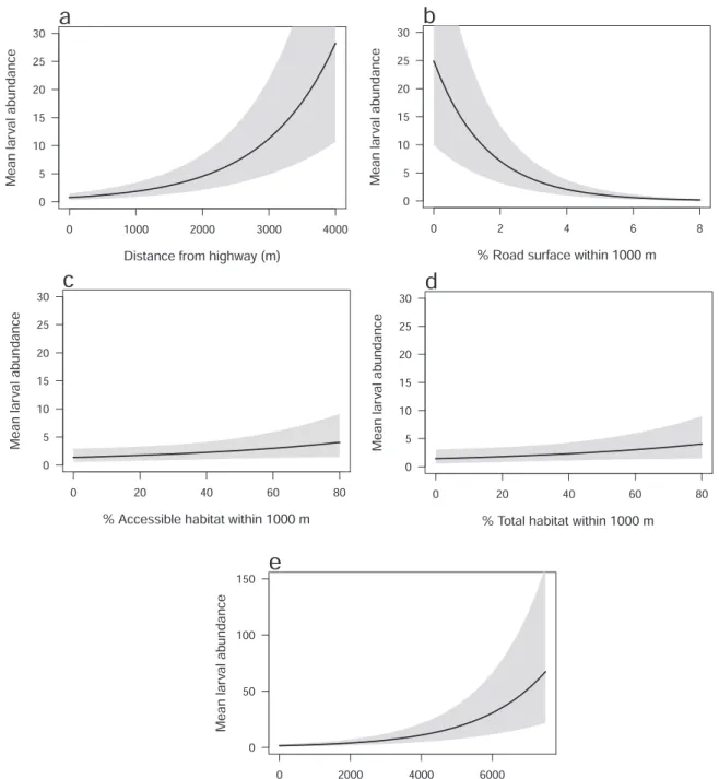
Mean community abundance (i.e. mean number of larvae) was predicted to increase from 0.77 at the site situated nearest to a highway (18 m), to 28.22 at the site located furthest from a highway (3869 m; Fig. 2a). There was only a small increase in abundance at sites located 0 – 1000 m from a highway suggesting that the road-effect zone extended for up to 1 km. There were relatively similar responses to Dist_hwy across all species in the community (σλ2 =0.486; Table 1). Mean abundance was predicted to decrease from Table 2
Summary of species-specific estimates for abundance (λ) and detection (β) covariates for the larvae of seven amphibian species. Estimates include 95% Bayesian credible intervals (BCI). Parameter estimates were extracted from the Dist_hwy model. Clear relationships are where the 95% BCI does not overlap zero (highlighted in bold, except intercept coefficients). SD =standard deviation.
Species Species-specific parameter Mean SD 95% BCI
Bombina bombina λ0 Intercept 1.389 0.487 0.463 2.349
(Family: Bombinatoridae) λ1 Area 2.249 0.220 1.821 2.684
λ2 Dist_hwy 1.644 0.321 1.017 2.280
λ3 Fish –2.129 0.248 –2.623 –1.650
β0 Intercept –4.288 0.370 –5.044 –3.580
β1 Water 1.148 0.100 0.956 1.348
β2 Temp –0.187 0.069 –0.322 –0.051
β3 Days 0.697 0.111 0.483 0.918
Bufo bufo λ0 Intercept 1.576 0.529 0.600 2.647
(Family: Bufonidae) λ1 Area 3.872 0.178 3.527 4.226
λ2 Dist_hwy 4.375 0.333 3.728 5.049
λ3 Fish –0.149 0.159 –0.458 0.162
β0 Intercept –5.411 0.286 –6.014 –4.884
β1 Water 1.006 0.065 0.879 1.134
β2 Temp –0.093 0.042 –0.175 –0.011
β3 Days 0.484 0.043 0.400 0.569
Hyla arborea λ0 Intercept 0.933 0.495 –0.077 1.888
(Family: Hylidae) λ1 Area 1.889 0.417 1.069 2.704
λ2 Dist_hwy 3.546 0.489 2.598 4.511
λ3 Fish –0.328 0.373 –1.072 0.387
β0 Intercept –4.181 0.461 –5.107 –3.299
β1 Water –0.001 0.181 –0.354 0.356
β2 Temp 0.657 0.195 0.286 1.051
β3 Days 1.641 0.264 1.145 2.180
Lissotriton vulgaris λ0 Intercept 1.078 0.483 0.103 2.033
(Family: Salamandridae) λ1 Area 1.452 0.334 0.798 2.106
λ2 Dist_hwy 2.147 0.389 1.391 2.920
λ3 Fish –0.069 0.293 –0.649 0.497
β0 Intercept –3.869 0.452 –4.770 –3.008
β1 Water 0.910 0.167 0.591 1.247
β2 Temp 0.393 0.137 0.128 0.663
β3 Days 0.921 0.169 0.595 1.257
Pelobates fuscus λ0 Intercept 1.013 0.489 0.029 1.981
(Family: Pelobatidae) λ1 Area 2.207 0.406 1.409 3.002
λ2 Dist_hwy 3.223 0.474 2.302 4.165
λ3 Fish –1.012 0.344 –1.697 –0.347
β0 Intercept –4.107 0.466 –5.029 –3.203
β1 Water 1.603 0.280 1.078 2.177
β2 Temp –0.488 0.161 –0.812 –0.177
β3 Days –0.203 0.222 –0.651 0.222
Pelophylax spp. complex λ0 Intercept 1.060 0.480 0.098 1.995
(Family: Ranidae) λ1 Area 1.323 0.262 0.818 1.843
λ2 Dist_hwy 0.955 0.304 0.363 1.556
λ3 Fish 3.490 0.281 2.950 4.057
β0 Intercept –5.878 0.323 –6.529 –5.257
β1 Water 2.913 0.186 2.552 3.280
β2 Temp 1.665 0.110 1.454 1.887
β3 Days 0.758 0.089 0.588 0.935
Rana dalmatina λ0 Intercept 1.370 0.519 0.426 2.464
(Family: Ranidae) λ1 Area 0.562 0.189 0.192 0.932
λ2 Dist_hwy 2.979 0.297 2.407 3.575
λ3 Fish 0.242 0.192 –0.135 0.621
β0 Intercept –4.560 0.353 –5.256 –3.871
β1 Water 0.306 0.058 0.194 0.421
β2 Temp –0.134 0.035 –0.202 –0.067
β3 Days –0.766 0.093 –0.952 –0.586
Area =pond area; Dist_hwy =distance to nearest highway; Fish =presence (1) or absence (0) of fish at a site; Water =% of full water-holding capacity at a site; Temp =water temperature; Days =number of days since 1 February 2020.
24.92 at the site with the lowest percentage cover of road surface within a 1000-m radius (0.04%), to 0.18 at the site with the highest road cover (7.03%; Fig. 2b).
Parameter estimates between mean community abundance and the landscape-scale covariates in the Access_hwy and Habitat models were similar (Table 1). Changes in mean community abundance relative to accessible habitat and total habitat were notably smaller than changes observed across the range of values for Dist_hwy and Roads. For example, mean community abundance was predicted to increase from 1.37 at the site with the lowest percentage of accessible habitat within a 1000-m radius, to 4.04 at the site with the highest percentage cover (Fig. 2c). Similarly, mean abundance was predicted to increase from 1.44 at the site with the lowest percentage of surrounding total habitat, to 4.05 at the site with the highest percentage cover of habitat (Fig. 2d).
There was a strong, clear positive relationship between mean community abundance and pond area (µArea =1.803, 95% BCI: 1.379
Fig. 2.Mean estimates of larval abundance (shaded areas are 95% Bayesian credible intervals) across the amphibian community versus five habitat covariates: (a) distance from highway; (b) % road surface within a 1000-m radius; (c) % accessible habitat within a 1000-m radius; (d) % total habitat within a 1000-m radius; and (e) pond area.
– 2.226; Table 1), which was also evident in the other five models (Table S5). Mean abundance was predicted to increase from 1.43 to 67.33 at the smallest and largest ponds, respectively (Fig. 2e). There was only a small increase in mean abundance at ponds with an area of 0 – 2000 m2. Responses to pond area were relatively similar across all species (σλ1 =0.482; Table 1).
There was a positive, but ambiguous, relationship between mean community abundance and fish presence, with the 95% BCI overlapping zero widely (µFish =0.154, 95% BCI: –0.273 to 0.584; Table 1). There was relatively high variability in species responses to the presence of fish (σλ3 =0.493; Table 1). Mean community abundance at sites with fish present was 3.36 (1.42 – 6.72) and 2.83 (1.35 – 5.23) at sites with no fish detected (Fig. S1).
There was positive and negative spatial autocorrelation in larval abundance at sites within nine of the 12 clusters (95% BCIs not overlapping zero), indicating that spatial position of ponds relative to other ponds affected larval community abundance (Fig. S2).
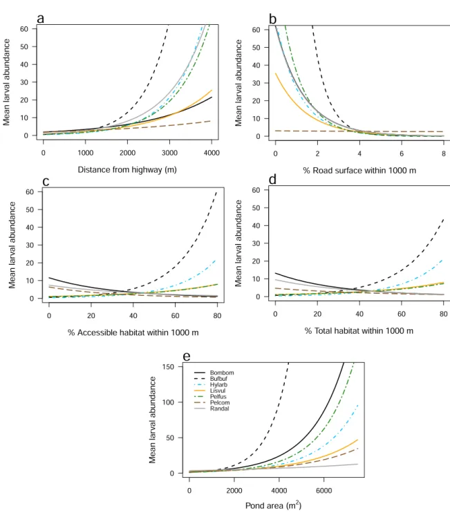
Fig. 3.Mean species-specific estimates of the larval abundance of seven amphibian species versus five habitat covariates: (a) distance from highway; (b) % road surface within a 1000-m radius; (c) % accessible habitat within a 1000-m radius; (d) % total habitat within a 1000-m radius;
and (e) pond area. Credible intervals are omitted for clarity. Species codes: Bombom =Bombina bombina; Bufbuf =Bufo bufo; Hylarb =Hyla arborea;
Lisvul =Lissotriton vulgaris; Pelfus =Pelobates fuscus; Pelcom =Pelophylax spp. complex; Randal =Rana dalmatina.
3.4. Larval species abundance
There was a clear positive relationship between the mean abundance of all seven species and distance to a highway (Fig. 3a), with the strongest and weakest relationships between the abundance of Bufo bufo larvae (λDist_hwy =4.375, 95% BCI: 3.728 – 5.049) and the Pelophylax spp. complex (λDist_hwy =0.955; 0.363 – 1.556; Table 2), respectively. Strong road effects were evident for all species at sites 0 - 1000 m from a highway, especially H. arborea, Pelobates fuscus and R. dalmatina (Fig. 3a). There was a clear negative relationship between the mean abundance of six species and the percentage cover of road surface within a 1000-m radius (Fig. 3b), although there was a weak and ambiguous relationship with the Pelophylax spp. complex (λRoads =–0.087; –0.555 to 0.368; Table S4). The strongest relationship between Roads and mean abundance was with Bufo bufo larvae (λRoads =–5.616; –6.282 to –5.008; Table S4).
There were mixed relationships between mean species abundance and percentage of accessible habitat within a 1000-m radius;
there was a clear positive relationship for Bufo bufo, H. arborea, L. vulgaris and Pelobates fuscus, whereas there were negative re- lationships for Bombina bombina, Pelophylax spp. complex and R. dalmatina (Fig. 3c; Table S4). There were similar relationships be- tween larval species abundance and percentage of total habitat (Fig. 3d; Table S4).
There was a clear positive relationship between mean species abundance and pond area (Table 2). The strongest relationship was for Bufo bufo larvae (λArea =3.872; 95% BCI: 3.527 – 4.226) whereas the weakest relationship was for R. dalmatina (λArea =0.562;
0.192 – 0.932; Fig. 3e; Table 2). There was also a positive relationship in the other five models (Table S4).
There was a clear negative relationship between the mean abundance of Bombina bombina and Pelobates fuscus larvae and fish presence, whereas there was a strong clear positive relationship with the Pelophylax spp. complex (Table 2; Fig. S1). Similar trends were evident in the other models; however, in the Roads model, there was a clear positive relationship between Bufo bufo larval abundance and fish presence, whereas there was a clear negative relationship with L. vulgaris (Table S4).
3.5. Detection probability
There were positive relationships between the community means for the probability of detection and site water levels, water temperature and the number of days since 1 February 2020 (Table 1; Table S5). There were positive relationships between the detection probabilities of six species and water levels (Table 2). Four species had clearly negative relationships between detection probability and water temperature, whereas three species had positive relationships (Table 2). There were positive relationships between detection probability and days since 1 February for five species (prolonged breeding species), while there was a negative relationship for R. dalmatina (early breeding species; Table 2).
4. Discussion
The effects of roads on amphibian populations can be severe and potentially wide-ranging (Beebee, 2013; Hamer et al. 2015). We provide evidence that roads are negatively affecting breeding communities of amphibian species in a landscape fragmented by agriculture and urbanisation. There were strong relationships between the mean abundance of larval amphibian communities and the distance to a highway and the extent of road cover within a 1000-m radius surrounding ponds. These relationships were stronger than the community responses to the proportion of accessible habitat and total habitat amount within a 1000-m radius. Although our study was conducted as a snap-shot over a single breeding season, the results suggest that the direct negative effects of roads have a stronger impact on amphibian abundance than the combined effects of roads and habitat amount in the study area. Our results concur with another study conducted in a rural landscape in eastern Europe which demonstrated that sealed roads with high traffic volumes (e.g.
highways) were the most important landscape elements influencing pond occupancy by amphibians, over and above the effects of landscape composition such as forest cover (Hartel et al. 2010). However, our study was conducted in an intensively-managed agricultural and peri-urban landscape, compared with the semi-natural rural landscape assessed by Hartel et al. (2010). As such, this is the first study to examine landscape-scale effects of habitat fragmentation and roads on amphibians in highly-modified land- scapes in central and eastern Europe.
4.1. Road and railway effects
Impacts of roads on wildlife often occur within road-effect zones over which significant ecological effects extend outward from a road for kilometres in some instances (Forman, 2000; Forman and Alexander, 1998; Forman and Deblinger, 2000). We present evi- dence for a road-effect zone extending up to 1 km from highways, in which ponds had a substantially lower abundance of amphibian larvae. Beebee (2013) documented road effects in amphibian communities occurring up to 2 km from roads. Highways can suppress amphibian reproduction in adjacent ponds and subsequently reduce population sizes of pond-breeding species because of road mortality (Beebee, 2013; Gibbs and Shriver, 2005; Karraker and Gibbs, 2011). As such, highways may be reducing amphibian pop- ulation viability in the study area via direct effects such as road mortality, through to indirect effects including traffic noise, modified hydrological patterns and contaminated runoff (Tennessen et al. 2014; Trombulak and Frissell, 2000).
We found interspecific differences in larval abundance occurring at distances >1 km from highways, with the strongest response evident for Bufo bufo, which displayed a strong negative relationship with road cover within a 1000-m radius around a pond. This species is highly vagile but moves relatively slowly during breeding migrations (Hels and Buchwald, 2001; Smith and Green, 2005).
These migrations are often intersected by roads and, consequently, Bufo bufo represents the highest percentage of road-killed am- phibians across much of Europe (Brzezi´nski et al. 2012; Hartel et al. 2009b; Hels and Buchwald, 2001). Eigenbrod et al. (2009)
detected road-effect zones extending up to 1 km from a highway in a rural landscape, with reduced abundances of four anuran species, but also found considerable variation among species. We found strong effects of roads for Hyla arborea, which responded negatively to roads and urbanisation at broad spatial scales (up to 1 km) in other fragmented European landscapes (e.g. Pellet et al. 2004a, b). Rana dalmatina responded negatively to roads and this species is susceptible to high rates of road mortality and reduced reproductive success in ponds surrounded by increasing urban land cover and high traffic roads (Hartel et al. 2009a, b). By comparison, there were no negative relationships between highways and roads for abundance of Pelophylax spp. complex larvae. While adult Pelophylax spp. are highly vagile (Smith and Green, 2005), it commonly inhabits urban ponds and highway stormwater ponds (Ficetola and De Bernardi, 2004; Herczeg et al. 2012; Le Viol et al. 2012). Furthermore, individuals remain at ponds throughout the breeding season, making them less susceptible to road traffic (Elzanowski et al. 2009).
There was no discernible effect of the main railway line on amphibian larval abundance, although there was some uncertainty in the parameter estimates, and this prediction requires further field testing. We initially predicted that the effect of the railway on amphibian abundance would be weaker than road effects, because railways generally have much lower traffic flow which is char- acterised by long traffic-free intervals, and railway corridors are narrower than highway corridors (Barrientos et al. 2019). None- theless, significant mortality rates can occur during the spring migration period in the vicinity of railway lines (e.g. Bufo bufo; Budzik and Budzik, 2014). Given that many aspects of railway ecology remain poorly researched, there is a need to collect more empirical data on the effects of railways on animal populations (Barrientos et al. 2019; Dorsey et al. 2015).
4.2. Accessible habitat
There was lower support for a model assessing the relationship between accessible habitat delineated by highways and amphibian abundance, although this model was better supported than one including only total area of habitat surrounding ponds. It would appear that highways are contributing to landscape fragmentation in the study area, most likely because they are barriers to breeding mi- grations, although there is some uncertainty in the magnitude of the effect. Similarly, landscape composition had a smaller effect on amphibian occurrence than the presence of high-traffic roads at distances up to 800 m in Romanian ponds (Hartel et al. 2010). In our study, Bufo bufo larval abundance was most strongly associated with both accessible habitat and total habitat within a 1000-m radius around a pond. Landscape composition surrounding ponds can affect breeding occupancy by Bufo bufo (Zanini et al. 2008) and connectivity with areas of high forest cover increases pond occupancy (Hartel et al. 2010). However, the smaller effect of accessible habitat on mean community abundance compared with distance to a highway may be that some features present in agricultural land surrounding ponds also supported terrestrial habitat for amphibians (e.g. hedgerows; Boissinot et al. 2019), but were not included in the calculation of accessible habitat. Our study was conducted in an intensively-managed agricultural/ peri-urban landscape, which may impede amphibian dispersal (Joly, 2019). Thus, existing disturbances and habitat modifications around ponds (e.g. agriculture;
Lenhardt et al. 2013) may have masked the impact of highways on amphibian abundance. Other studies assessing accessible habitat as a predictor of amphibian occupancy were conducted in less-urbanised landscapes (e.g. Eigenbrod et al. 2008b; Hamer, 2016). Future studies of the impacts of roads using accessible habitat as a predictor variable may uncover a greater effect if they are restricted to more rural areas.
One limitation of our measure of accessible habitat was that there was often only a small fraction of habitat on the opposite side of a highway (see Fig. 1). As such, there was only a minor difference between the mean area of total habitat and accessible habitat in the study area (Table S1), making it potentially difficult to separate the effects of the highways from total habitat area on amphibian abundance. Our measure of habitat included both forest and wetland, and there are likely to be differences among species in habitat usage; e.g. Bufo bufo and Rana dalmatina are more likely to inhabit forests during the non-breeding period, whereas Bombina bombina and the Pelophylax spp. complex members often remain within the pond vicinity throughout the breeding season (Elzanowski et al.
2009). Further delineation of accessible habitat between habitat types may be required in future studies to determine the relative contribution of forests and wetlands to landscape permeability for amphibians around ponds. For example, the amount of forest in a landscape may be more important than the amount of wetland (Quesnelle et al. 2015).
4.3. Importance of local habitat
The abundance of larval amphibians was strongly related to pond area, with a clear consistent relationship evident across all species. This result aligns with the metapopulation theory that larger patch sizes will support a greater abundance of species (Hanski, 1994). Larger ponds provide greater habitat heterogeneity and resources for aquatic species (Zedler and Kercher, 2005), and larger ponds in the study area had a longer hydroperiod that may increase the probability of individuals reaching metamorphosis (Table S2).
There were mixed relationships between fish presence and the abundance of larvae, which likely reflect the range of species’ life histories and adaptations to co-exist with fish (Wellborn et al. 1996). There were clear negative relationships between fish presence and the abundance of Bombina bombina and Pelobates fuscus larvae, which may not possess adaptations to avoid fish predation. For instance, Bombina bombina larvae occur predominantly in fishless ponds (Kloskowski et al. 2020), and the abundance of Pelobates fuscus larvae was negatively correlated with fish presence in other agricultural landscapes (Rannap et al. 2015). There was a strong asso- ciation of larvae of the Pelophylax spp. complex with fish presence, which may co-exist successfully with fish because their larvae display morphological and behavioural responses to fish predators (Hartel et al. 2007; Kloskowski et al. 2020; Teplitsky et al. 2003).