agriculture
Article
Crop Productivity and Climatic Conditions: Evidence from Hungary
Zoltán Bakucs1,* , Imre Fert ˝o1,2 and Enik ˝o Vígh3,4
1 Institute of Economics, Centre for Economic and Regional Studies, 1097 Budapest, Tóth Kálmán u. 4., Hungary;
ferto.imre@krtk.mta.hu
2 Doctoral School in Management and Organizational Sciences, Kaposvár Campus, Szent István University, 7400 Kaposvár, Guba Sándor u. 40., Hungary
3 NARIC Research Institute of Agricultural Economics, 1093 Budapest, Zsil utca 3–5., Hungary;
vigh.eniko.zita@aki.naik.hu
4 Department of Economics, Partium Christian University, 410209 Oradea, Str. Primăriei, Nr. 36, Romania
* Correspondence: zoltan.bakucs@krtk.mta.hu
Received: 1 September 2020; Accepted: 20 September 2020; Published: 22 September 2020
Abstract: Hungarian agriculture is expected to experience greater risks due to more variability in crop productivity due to increasing yearly average temperatures and extreme precipitation patterns.
This study investigates the effect of changing climatic conditions on productivity, using a Hungarian sample of crop producers for a 12-year time period. Our empirical analysis employs True Fixed Effects frontier models of Farm Accountancy Data Network data that are merged with specific meteorological data representatively maintained for seeding, vegetative, and generative periods for cereals, oil seed and protein crops, along with soil quality and usage-related data. Estimations indicate that climate variables have significant impacts on technical efficiency. In addition, calculation suggest that an increase in temperature during seeding and vegetative periods, combined with higher precipitation levels in May and June, will reduce crop farmers’ production frontier. Estimations explain the variance, while the technical efficiency (TE) scores emphasize the impact of the difference in soil quality and its water absorption capacity.
Keywords: climatic effects; crop production; technical efficiency; SFA; Hungary
1. Introduction
Several papers investigate the effects of climate change on European agriculture [1–6], and their conclusions suggest a range of different outcomes. Most research concludes that climate variability is an important factor to negatively influence crop production [2,6]. However, other studies conclude that global warming has improved agro-climatic conditions in many regions of Europe [1,3–5]. All the research agrees, however, that in one way or another climate change is very likely to influence the productivity in agriculture.
Although there are many papers on efficiency in agriculture, research into the link between climate change and the technical efficiency of farms [7–11] that has focused on countries outside Europe (Australia, Chile, and the USA) is limited. Some of the reviewed results suggest that negative association exists between climatic effects and dairy farm output [7,9], others find that average temperature has a positive impact on dairy production [10,11] while average temperature in winter time has no significant impact [10]. The literature also highlights that based on applied method the results can be substantially different [8]. This paper extends this literature to crop production in Europe, more specifically, to Hungary.
Agriculture2020,10, 421; doi:10.3390/agriculture10090421 www.mdpi.com/journal/agriculture
In this paper, we focus on Hungarian crop production. To briefly emphasize the sector’s importance, it amounts to 58% of total agricultural gross output, and contributes at least HUF 2410 billion to the Hungarian economy. The paper is structured as follows: Section1presents climatic trends in Hungary;
Section2contains information about the data and methodological specifications. Section3presents results based on stochastic frontier-, true fixed-, and random effect models. Section4describes the discussion of the results.
Temperature and Precipitation Trends in Hungary
Hungary is a located in a geographical region associated with the greatest uncertainty with respect to climate projections [12,13]. In the last century, the climatic change has been characterized by warming, which has accelerated due to growing anthropogenic influence since the 1970s. The Hungarian Meteorological Service reports an increase in the number of heat days and a fall in the number of frost days. Climate-change-induced temperature extremes are growing faster than the average temperature.
Heat wave intensity, length and frequency have grown in the South-East European region [14].
The Carpathian region is also subject to climate change due to weather-related extremes [15,16].
For example, the summer of 2012 was characterized by serious rainfalls which led to flooding in Northern Europe and droughts and wildfires in Southern Europe [17]. In the period 1921–1999 in Western Europe, there were significant and extreme precipitation patterns [14,18], which also occurred in Hungary. An increase in the threat of extreme variability in precipitation that affects irrigation and soil erosion may be expected. Further, in the period 1961–1990, temperature anomalies and exceptionally low precipitation levels were recorded [17]. There were two floods (the Tisza and the Danube in 2006) and considerable damage to inlands was caused by excess water and flooding [19].
According to changing climate patterns, we can distinguish four main climate-regions [20].
The frequency, duration, and average intensity of climate-change-driven drought events in the Carpathian region will increase [15]. Meteorological estimations indicate that most changes will occur over the continental area both in summer and winter, although the distribution of projected precipitation will be asymmetrical and, in some cases, oppositional in the two seasons (a decrease in summer and an increase in winter). According to the PRECIS (Hadley Centre at the UK Met Office, Exeter, UK) [21] regional climate model simulations, year-on-year variation in Hungary will significantly change in the future, while (simulated) precipitation changes in the transition seasons involve major uncertainty. The drying tendency shows that it is mainly the south-eastern part of the country that may face the serious drought hazard [20].
In sum, over recent decades, considerable changes in the climatic conditions of Hungary have been observed, with variability in temperature and precipitation. These projections reinforce the likelihood of the continuation of significant change in the climate of Hungary.
2. Materials and Methods
2.1. Data
We use an extended Farm Accountancy Data Network (FADN) panel dataset from 2002–2013 for crop-producing farms in Hungary. Along with classic production function estimation procedures, we use output measured as value of gross production as sum of the total incomes and capitalized own performance (HUF 1000, deflated) and four inputs: land as sum of kitchen garden, productive land and uncultivated land (measured in hectares), labor as regular and casual paid labor expressing total agricultural activity (Annual Work Unit, AWU), capital as total net worth calculated from subscribed capital, unpaid subscribed capital, accumulated profit reserve and balance sheet (HUF 1000, deflated), and intermediate consumption expressed as sum of material costs, main costs, other material costs of the agricultural activity not yet accounted for, material costs in forest management and material costs in game management (HUF 1000, deflated). Meteorological data were obtained from the EU Joint Research Centre, MARS-AGRI4CAST [22] project—namely, daily average temperature (◦C), sum of precipitation
(mm/day) for seeding (April), vegetative (May–June), and generative (July–August) periods. Additional dummy variables used to control for soil quality and limitation of land use include (EU Joint Research Center, EUSOILS) [23]: AGRICUL—denotes the dominant limitations for the agricultural use of soils, HWC_SUB—denotes the water-absorbing capacity of subsoil, where>140 mm/m is considered soil with good water retention capacity. HWC_TOP describes the water retention capacity of topsoil, while finally the LOC_TOP variable denotes soil organic content, where<2% organic content is considered low-organic-content topsoil. We also consider additional variables such as the legal structure of farms. Legal as a dummy variable takes the value one if the farm is a corporate farm and zero for individual farms.
Throughout the observed period, yearly temperature and rainfall data vary greatly amongst Hungarian regions. Thus, a start–end period comparison would not reveal any robust information in this respect. The average meteorological variables throughout the period on a LAU1 (Local Administrative Unit, level 1, formerly known as NUTS4) disaggregation level are shown in Figures1 and2. The different geographical areas (e.g., the Great Hungarian Plain) are clearly visible, as is the disparity between temperature and rainfall.
Agriculture 2020, 10, x FOR PEER REVIEW 3 of 11
generative (July–August) periods. Additional dummy variables used to control for soil quality and limitation of land use include (EU Joint Research Center, EUSOILS) [23]: AGRICUL—denotes the dominant limitations for the agricultural use of soils, HWC_SUB—denotes the water-absorbing capacity of subsoil, where >140 mm/m is considered soil with good water retention capacity.
HWC_TOP describes the water retention capacity of topsoil, while finally the LOC_TOP variable denotes soil organic content, where <2% organic content is considered low-organic-content topsoil.
We also consider additional variables such as the legal structure of farms. Legal as a dummy variable takes the value one if the farm is a corporate farm and zero for individual farms.
Throughout the observed period, yearly temperature and rainfall data vary greatly amongst Hungarian regions. Thus, a start–end period comparison would not reveal any robust information in this respect. The average meteorological variables throughout the period on a LAU1 (Local Administrative Unit, level 1, formerly known as NUTS4) disaggregation level are shown in Figures 1 and 2. The different geographical areas (e.g., the Great Hungarian Plain) are clearly visible, as is the disparity between temperature and rainfall.
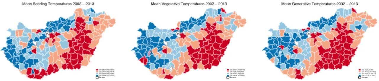
Figure 1. Mean seeding, vegetative and generative temperatures on a Local Administrative Unit Level 1 (LAU1). Source: authors’ calculations based on EU Joint Research Center MARS-AGRI4CAST [22].
Figure 2. Mean seeding, vegetative and generative precipitation on a LAU1 level. Source: authors’
calculations based on EU Joint Research Center MARS-AGRI4CAST [22].
Figures 1 and 2 reveal that high-temperature and higher precipitation regions do not overlap, emphasizing the challenges Hungarian agriculture is facing. The highest temperature rise is experienced in the southern part of the country, where the widest variation of precipitation is also observed. The precipitation distribution over time is also challenging, the regions experiencing water shortage in seeding and vegetative periods encounter water surplus in generative phase, which may result in deterioration of quality in harvested yields.
The descriptive statistics of climatic variables highlight serious variability in climatic conditions (Table 1).
Figure 1.Mean seeding, vegetative and generative temperatures on a Local Administrative Unit Level 1 (LAU1). Source: authors’ calculations based on EU Joint Research Center MARS-AGRI4CAST [22].
Agriculture 2020, 10, x FOR PEER REVIEW 3 of 11
generative (July–August) periods. Additional dummy variables used to control for soil quality and limitation of land use include (EU Joint Research Center, EUSOILS) [23]: AGRICUL—denotes the dominant limitations for the agricultural use of soils, HWC_SUB—denotes the water-absorbing capacity of subsoil, where >140 mm/m is considered soil with good water retention capacity.
HWC_TOP describes the water retention capacity of topsoil, while finally the LOC_TOP variable denotes soil organic content, where <2% organic content is considered low-organic-content topsoil.
We also consider additional variables such as the legal structure of farms. Legal as a dummy variable takes the value one if the farm is a corporate farm and zero for individual farms.
Throughout the observed period, yearly temperature and rainfall data vary greatly amongst Hungarian regions. Thus, a start–end period comparison would not reveal any robust information in this respect. The average meteorological variables throughout the period on a LAU1 (Local Administrative Unit, level 1, formerly known as NUTS4) disaggregation level are shown in Figures 1 and 2. The different geographical areas (e.g., the Great Hungarian Plain) are clearly visible, as is the disparity between temperature and rainfall.
Figure 1. Mean seeding, vegetative and generative temperatures on a Local Administrative Unit Level 1 (LAU1). Source: authors’ calculations based on EU Joint Research Center MARS-AGRI4CAST [22].
Figure 2. Mean seeding, vegetative and generative precipitation on a LAU1 level. Source: authors’
calculations based on EU Joint Research Center MARS-AGRI4CAST [22].
Figures 1 and 2 reveal that high-temperature and higher precipitation regions do not overlap, emphasizing the challenges Hungarian agriculture is facing. The highest temperature rise is experienced in the southern part of the country, where the widest variation of precipitation is also observed. The precipitation distribution over time is also challenging, the regions experiencing water shortage in seeding and vegetative periods encounter water surplus in generative phase, which may result in deterioration of quality in harvested yields.
The descriptive statistics of climatic variables highlight serious variability in climatic conditions (Table 1).
Figure 2. Mean seeding, vegetative and generative precipitation on a LAU1 level. Source: authors’
calculations based on EU Joint Research Center MARS-AGRI4CAST [22].
Figures1and2reveal that high-temperature and higher precipitation regions do not overlap, emphasizing the challenges Hungarian agriculture is facing. The highest temperature rise is experienced in the southern part of the country, where the widest variation of precipitation is also observed.
The precipitation distribution over time is also challenging, the regions experiencing water shortage in seeding and vegetative periods encounter water surplus in generative phase, which may result in deterioration of quality in harvested yields.
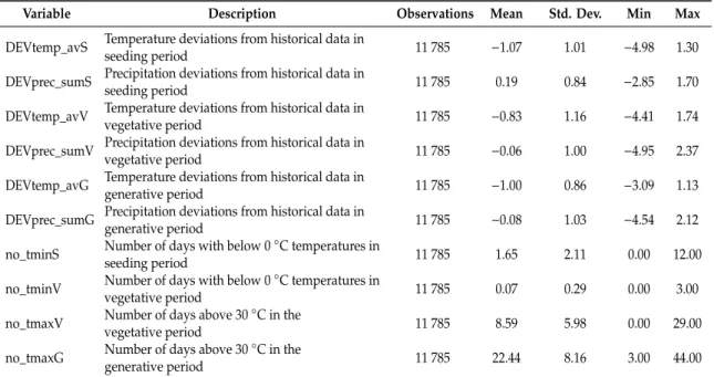
The descriptive statistics of climatic variables highlight serious variability in climatic conditions (Table1).
Table 1.Descriptive statistics of variables for 2002–2013.
Variable Description Observations Mean Std. Dev. Min Max
DEVtemp_avS Temperature deviations from historical data in
seeding period 11 785 −1.07 1.01 −4.98 1.30
DEVprec_sumS Precipitation deviations from historical data in
seeding period 11 785 0.19 0.84 −2.85 1.70
DEVtemp_avV Temperature deviations from historical data in
vegetative period 11 785 −0.83 1.16 −4.41 1.74
DEVprec_sumV Precipitation deviations from historical data in
vegetative period 11 785 −0.06 1.00 −4.95 2.37
DEVtemp_avG Temperature deviations from historical data in
generative period 11 785 −1.00 0.86 −3.09 1.13
DEVprec_sumG Precipitation deviations from historical data in
generative period 11 785 −0.08 1.03 −4.54 2.12
no_tminS Number of days with below 0◦C temperatures in
seeding period 11 785 1.65 2.11 0.00 12.00
no_tminV Number of days with below 0◦C temperatures in
vegetative period 11 785 0.07 0.29 0.00 3.00
no_tmaxV Number of days above 30◦C in the
vegetative period 11 785 8.59 5.98 0.00 29.00
no_tmaxG Number of days above 30◦C in the
generative period 11 785 22.44 8.16 3.00 44.00
Temperature is measured in Celsius, precipitation in mm/day. Source: authors’ calculations
The following variables were defined to create the inefficiency function—all were observed in the grid in which the farm operates:
1. Number of extreme temperature days: no_tminS and no_tminV: number of days with below 0◦C temperatures in Seeding and Vegetative periods, respectively; no_tmaxV and no_tmaxG: number of days above 30◦C in the Vegetative and Generative periods, respectively.
2. Deviations from long-run, historical temperature and precipitation. To calculate deviations, we employed grid-specific daily weather data from 1975–2013. Thus, DEVtemp_avS, DEVtemp_avV, DEVtemp_avG denote temperature deviations, whilst DEVprec_sumS, DEVprec_sumV, DEVprec_sumG denote precipitation deviations from historical data in Seeding, Vegetative and Generative periods, respectively.
3. Deviations from historical extreme weather events.
The first step of our investigation was to estimate technical efficiency (TE) scores. Since Schmidt and Knox-Lovell [24] and Meeusen and van den Broeck [25], stochastic frontier analysis has become a standard tool in applied economics. Standard efficiency models assume that all firms face a common frontier and differences only result from the intensity of input use [26,27]. A fundamental role of stochastic frontier models is to estimate the technical (cost) inefficiency exploiting the conditional distribution of the error term [28].
2.2. Method
Panel data models including fixed-effects or random-effects models are appropriate to account for unobserved heterogeneity [29,30]. There are two major shortcomings of these models: (i) treating the inefficiency term as time-invariant, which causes a fundamental identification problem, and (ii) the fact that they are not able to distinguish between cross-individual heterogeneity and inefficiency [31,32].
To solve these shortcomings, Greene [32] suggests two stochastic frontier models that are time-variant and that distinguish unobserved heterogeneity from the inefficiency component. These models are called the “true” fixed-effects- (TFE) and “true” random effects (TRE) models. Greene [32] notes that the TFE model may produce biased individual effects and efficiency estimates due to the presence of individual effects creating an incidental parameter problem. However, TRE models produce unbiased inefficiency estimates, yet require stronger assumptions. Since current climatic conditions are
incorporated into the TRANSLOG frontier, one could argue that departures from long-term conditions or extreme weather events may impact technical efficiency scores. The TRE model can be specified as:
yit=α+ f xit:β
+wi+vit−uit (1) whereyit is the log of output (value of production) for farmiat timet; αis a common intercept;
f(xit:β) is the production technology;xitis the vector of inputs (in logs);βis the associated vector of technology parameters to be estimated;wiis a time invariant and farm specific random term to capture unobserved heterogeneity;vitis a random two-sided noise term (exogenous production shocks) that can increase or decrease output (ceteris paribus); anduit>0 is the non-negative, one-sided inefficiency term. The parameters of the model are estimated using the maximum likelihood (ML) method with the following distributional assumptions:
uit~N+(0,σ2u) (2)
vit~N+(0,σ2v) (3)
wi~N+(0,σ2w) (4)
whereN+expresses the positive normal distribution, 0 is the expected value;σ2uis the variance ofu;
σ2vis the variance ofvandσ2wis the variance ofw, respectively.
To predict farm-specific technical efficiency we apply an estimator from Battese and Coelli [33].
There are two main approaches [34] to accounting for meteorological data in production functions.
The first one estimates efficiency scores and regresses the result on climate data (e.g., [35]), implicitly assuming that climate data changes efficiency. The second approach, which we follow in this paper, considers climate effects as non-material inputs that enter the production function (e.g., [7,9,36]).
To examine the different assumptions of our analysis we compared five specifications of SFA (Stochastic Frontier Analysis) models, where Model 1=pooled frontier without climatic variables;
Model 2=pooled frontier with climatic variables; Model 3=TFE specification with climatic variables;
Model 4= TRE specification with climatic variables; and Model 5=TRE model with Mundlak’s specification and climatic variables and climatic variables. Models 1 and 2 essentially treat the data as cross-sectional, whereas Models 3 to 5 use panel data treatment.
3. Results
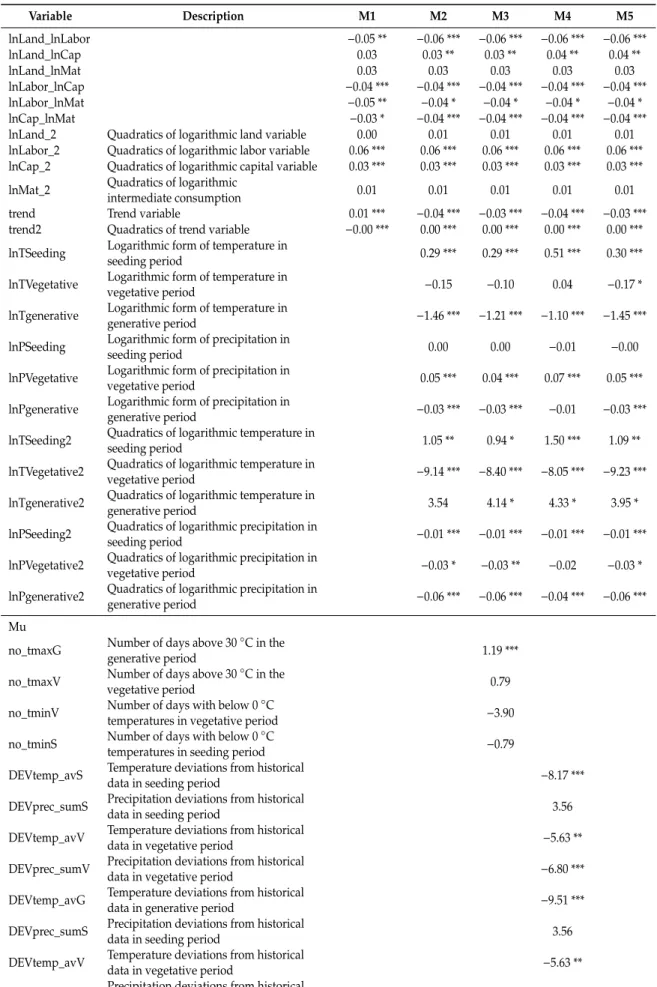
Based on data about Hungarian plant producers from 2003 to 2013, the research described herein constructed SFA and TFE models to estimate the technical efficiencies of the sample. Table2shows parameter estimates from the stochastic frontier models.
Table 2.Estimation Results.
Variable Description M1 M2 M3 M4 M5
Frontier
lnLand Logarithmic form of land variable 0.00 0.01 0.01 0.02 0.01
lnLabor Logarithmic form of labor variable 0.08 *** 0.09 *** 0.09 *** 0.08 *** 0.09 ***
lnCap Logarithmic form of capital variable 0.09 *** 0.09 *** 0.09 *** 0.08 *** 0.09 ***
lnMat Logarithmic form of
intermediate consumption 0.83 *** 0.82 *** 0.82 *** 0.82 *** 0.82 ***
lnLand_lnLabor −0.05 ** −0.06 *** −0.06 *** −0.06 *** −0.06 ***
lnLand_lnCap 0.03 0.03 ** 0.03 ** 0.04 ** 0.04 **
lnLand_lnMat 0.03 0.03 0.03 0.03 0.03
lnLabor_lnCap −0.04 *** −0.04 *** −0.04 *** −0.04 *** −0.04 ***
lnLand_lnLabor −0.05 ** −0.06 *** −0.06 *** −0.06 *** −0.06 ***
lnLand_lnCap 0.03 0.03 ** 0.03 ** 0.04 ** 0.04 **
lnLand_lnMat 0.03 0.03 0.03 0.03 0.03
Table 2.Cont.
Variable Description M1 M2 M3 M4 M5
lnLand_lnLabor −0.05 ** −0.06 *** −0.06 *** −0.06 *** −0.06 ***
lnLand_lnCap 0.03 0.03 ** 0.03 ** 0.04 ** 0.04 **
lnLand_lnMat 0.03 0.03 0.03 0.03 0.03
lnLabor_lnCap −0.04 *** −0.04 *** −0.04 *** −0.04 *** −0.04 ***
lnLabor_lnMat −0.05 ** −0.04 * −0.04 * −0.04 * −0.04 *
lnCap_lnMat −0.03 * −0.04 *** −0.04 *** −0.04 *** −0.04 ***
lnLand_2 Quadratics of logarithmic land variable 0.00 0.01 0.01 0.01 0.01
lnLabor_2 Quadratics of logarithmic labor variable 0.06 *** 0.06 *** 0.06 *** 0.06 *** 0.06 ***
lnCap_2 Quadratics of logarithmic capital variable 0.03 *** 0.03 *** 0.03 *** 0.03 *** 0.03 ***
lnMat_2 Quadratics of logarithmic
intermediate consumption 0.01 0.01 0.01 0.01 0.01
trend Trend variable 0.01 *** −0.04 *** −0.03 *** −0.04 *** −0.03 ***
trend2 Quadratics of trend variable −0.00 *** 0.00 *** 0.00 *** 0.00 *** 0.00 ***
lnTSeeding Logarithmic form of temperature in
seeding period 0.29 *** 0.29 *** 0.51 *** 0.30 ***
lnTVegetative Logarithmic form of temperature in
vegetative period −0.15 −0.10 0.04 −0.17 *
lnTgenerative Logarithmic form of temperature in
generative period −1.46 *** −1.21 *** −1.10 *** −1.45 ***
lnPSeeding Logarithmic form of precipitation in
seeding period 0.00 0.00 −0.01 −0.00
lnPVegetative Logarithmic form of precipitation in
vegetative period 0.05 *** 0.04 *** 0.07 *** 0.05 ***
lnPgenerative Logarithmic form of precipitation in
generative period −0.03 *** −0.03 *** −0.01 −0.03 ***
lnTSeeding2 Quadratics of logarithmic temperature in
seeding period 1.05 ** 0.94 * 1.50 *** 1.09 **
lnTVegetative2 Quadratics of logarithmic temperature in
vegetative period −9.14 *** −8.40 *** −8.05 *** −9.23 ***
lnTgenerative2 Quadratics of logarithmic temperature in
generative period 3.54 4.14 * 4.33 * 3.95 *
lnPSeeding2 Quadratics of logarithmic precipitation in
seeding period −0.01 *** −0.01 *** −0.01 *** −0.01 ***
lnPVegetative2 Quadratics of logarithmic precipitation in
vegetative period −0.03 * −0.03 ** −0.02 −0.03 *
lnPgenerative2 Quadratics of logarithmic precipitation in
generative period −0.06 *** −0.06 *** −0.04 *** −0.06 ***
Mu
no_tmaxG Number of days above 30◦C in the
generative period 1.19 ***
no_tmaxV Number of days above 30◦C in the
vegetative period 0.79
no_tminV Number of days with below 0◦C
temperatures in vegetative period −3.90
no_tminS Number of days with below 0◦C
temperatures in seeding period −0.79
DEVtemp_avS Temperature deviations from historical
data in seeding period −8.17 ***
DEVprec_sumS Precipitation deviations from historical
data in seeding period 3.56
DEVtemp_avV Temperature deviations from historical
data in vegetative period −5.63 **
DEVprec_sumV Precipitation deviations from historical
data in vegetative period −6.80 ***
DEVtemp_avG Temperature deviations from historical
data in generative period −9.51 ***
DEVprec_sumS Precipitation deviations from historical
data in seeding period 3.56
DEVtemp_avV Temperature deviations from historical
data in vegetative period −5.63 **
DEVprec_sumV Precipitation deviations from historical
data in vegetative period −6.80 ***
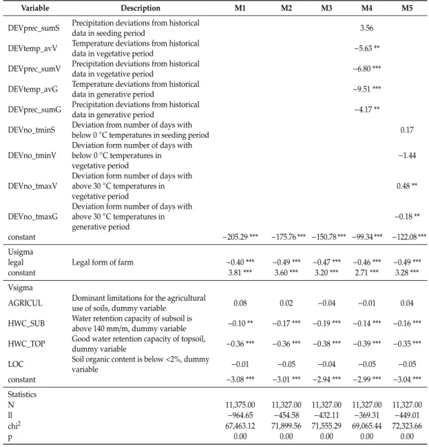
Table 2.Cont.
Variable Description M1 M2 M3 M4 M5
DEVprec_sumS Precipitation deviations from historical
data in seeding period 3.56
DEVtemp_avV Temperature deviations from historical
data in vegetative period −5.63 **
DEVprec_sumV Precipitation deviations from historical
data in vegetative period −6.80 ***
DEVtemp_avG Temperature deviations from historical
data in generative period −9.51 ***
DEVprec_sumG Precipitation deviations from historical
data in generative period −4.17 **
DEVno_tminS Deviation from number of days with
below 0◦C temperatures in seeding period 0.17
DEVno_tminV
Deviation form number of days with below 0◦C temperatures in vegetative period
−1.44
DEVno_tmaxV
Deviation form number of days with above 30◦C temperatures in vegetative period
0.48 **
DEVno_tmaxG
Deviation form number of days with above 30◦C temperatures in generative period
−0.18 **
constant −205.29 *** −175.76 *** −150.78 *** −99.34 *** −122.08 ***
Usigma
legal Legal form of farm −0.40 *** −0.49 *** −0.47 *** −0.46 *** −0.49 ***
constant 3.81 *** 3.60 *** 3.20 *** 2.71 *** 3.28 ***
Vsigma
AGRICUL Dominant limitations for the agricultural
use of soils, dummy variable 0.08 0.02 −0.04 −0.01 0.04
HWC_SUB Water retention capacity of subsoil is
above 140 mm/m, dummy variable −0.10 ** −0.17 *** −0.19 *** −0.14 *** −0.16 ***
HWC_TOP Good water retention capacity of topsoil,
dummy variable −0.36 *** −0.36 *** −0.38 *** −0.39 *** −0.35 ***
LOC Soil organic content is below<2%, dummy
variable −0.01 −0.05 −0.04 −0.05 −0.05
constant −3.08 *** −3.01 *** −2.94 *** −2.99 *** −3.04 ***
Statistics
N 11,375.00 11,327.00 11,327.00 11,327.00 11,327.00
ll −964.65 −454.58 −432.11 −369.31 −449.01
chi2 67,463.12 71,899.56 71,555.29 69,065.44 72,323.66
p 0.00 0.00 0.00 0.00 0.00
*p<0.10, *p<0.05, ***p<0.01; Source: authors’ calculations.
Variables that control the production frontier (lnLabor, lnCap, lnMat) are significant and they have expected positive signs and values. Similarly, the coefficients for farm expenditures were consistent with the others in the pooled models. The time trend, which was incorporated into the production frontier to reflect technological progress, was statistically significant with a positive effect.
The first group of meteorological variables examined the effect of temperature and precipitation values measured in sowing, vegetative, and generative phenological phases on farm efficiency.
Higher temperatures measured during the sowing (Tseeding) period have a positive effect on efficiency.
The result is not surprising, as we assume that the sowing period of the continental climate belt can be made in April, during which time higher temperatures are essential for the germination of spring-sown plants. The effect of changes in precipitation patterns over the same period is not clear. While for M2 and M3 specifications the increase in precipitation has a positive effect, for M4 and M5 it has reduced efficiency. The results are explained by the fact that rainfall distribution is a key issue in outdoor crop production, the mere increase in higher rainfall does not improve yields, and the temporal and spatial distribution of falling precipitation images is difficult to predict.
There is a change of sign in the vegetative (Tvegetative) and generative (Tgenerative) periods.
The phenologically important plant growth or vegetation period can occur in May-June, during which time the vegetative parts of the plants are formed, for example when the stems and leaves are formed.
The higher temperature in most cases significantly and negatively affected the change in efficiency in most model specifications. The results show that higher precipitation measured during the growth period improved the efficiency of the surveyed plants.
The ripening and harvest period can occur in July-August; during this period the increase in temperature (Tgenerative) greatly and significantly impaired the efficiency. The results of the square members show that the relationship is not linear. Increased precipitation (Pgenerative) also suggests a negative effect. The results are based on the effects of yields on harvest quality, as the sudden rise in temperature and falling precipitation degrade the marketability and quality characteristics of the produce for most crops.
The second part of the table (Mu) contains the factors determining inefficient operation.
Cold stress and heat stress, which are becoming more frequent as a result of climate change, are the environmental factors that most reduce plant production through disruption of molecular, biochemical and physiological processes. Heat stress affects plant nutrient uptake, nutrient utilization, development of vegetative parts, intensity of photosynthesis and respiration, yield, and yield quality.
Low temperatures are critical for plants, as they are one of the most important determinants of the occurrence and prevalence of natural plant associations. In the case of agricultural cultivation, temperature is the factor that most limits the ability of plants to grow in a given area. As a result of cold stress, the development of the plant is significantly slowed down and physiologically damaged, the number of germinating seeds is reduced, and the time required for germination is lengthened.
Cold stress in young plants significantly reduces the photosynthetic activity of the plant, which is reflected in both a decrease in CO2assimilation and a slowdown in photosynthetic processes. In the studied 12-year period, we examined the number of days where the average daily temperature was below 0◦C (cold stress) or above 30◦C (heat stress), separately to the values measured in the sowing (S), vegetative (V) and generative (G) periods. The number of heat stress days significantly explains the lack of efficiency in the generative period, heat stress worsened the output of crop growers during the crop period. Inefficient functioning also increases during the vegetative (growth) period.
Climate change studies often evaluate differences in meteorological values from the base period.
The M4 model examines the differences in the average temperature and precipitation amount within the country, where the period of comparison is given as the period between 1975 and 2013. In all three study periods, deviations from long-term temperature experiences significantly reduced effective status, which can be explained by the adaptive behavior of farmers who monitor long-term meteorological changes and take steps to reduce expected negative effects. The evolution of precipitation patterns is not so clear. Decreasing efficiency in the sowing phase changes by significantly decreasing results in the vegetative and generative phases.
In addition to climate change, the model includes the characteristic soil quality factors of the plants based on the ESDAC EUSOILS data, namely the water holding capacity of the sub- and topsoil and the organic matter content. Soil quality coefficients influencing Vsigma variance are significant and well-characterized. In most model specifications, the high water management capacity of soils increases plant efficiency. The effect of the legal form defining Usigma variance has yielded significant results. The results show that the inefficient state decreases in the case of individual farms, while in the case of ceteris paribus, the ineffective state is more common in all examined model specifications.
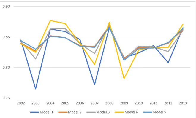
Figure3shows the mean annual TE estimated from each model. Average TE for model 4, which fits the best, was 0.840. Average TE for Models 2 to 5 were higher than for Model 1 which is consistent with the fact that the climate variables have important effect on TE.
Agriculture2020,10, 421 9 of 12
Climate change studies often evaluate differences in meteorological values from the base period.
The M4 model examines the differences in the average temperature and precipitation amount within the country, where the period of comparison is given as the period between 1975 and 2013. In all three study periods, deviations from long-term temperature experiences significantly reduced effective status, which can be explained by the adaptive behavior of farmers who monitor long-term meteorological changes and take steps to reduce expected negative effects. The evolution of precipitation patterns is not so clear. Decreasing efficiency in the sowing phase changes by significantly decreasing results in the vegetative and generative phases.
In addition to climate change, the model includes the characteristic soil quality factors of the plants based on the ESDAC EUSOILS data, namely the water holding capacity of the sub- and topsoil and the organic matter content. Soil quality coefficients influencing Vsigma variance are significant and well-characterized. In most model specifications, the high water management capacity of soils increases plant efficiency. The effect of the legal form defining Usigma variance has yielded significant results. The results show that the inefficient state decreases in the case of individual farms, while in the case of ceteris paribus, the ineffective state is more common in all examined model specifications.
Figure 3 shows the mean annual TE estimated from each model. Average TE for model 4, which fits the best, was 0.840. Average TE for Models 2 to 5 were higher than for Model 1 which is consistent with the fact that the climate variables have important effect on TE.
Figure 3. Average annual technical efficiency (%) estimated for each model. Source: authors’
calculations.
4. Discussion
Understanding climatic impacts on the technical efficiency of agricultural crop production is of central importance. Thus, we employed climatic (MARS Agri4cast) and soil (ESDAC EUSOILS) variables in alternative stochastic production frontier models to derive measures of climatic effects based on a representative Hungarian plant-producer dataset (FADN) from 2002 to 2013. Many of the underlying drivers of the negative effects of climate change are subject to uncertainty. Meteorological events are not easily predictable beyond a few decades, and economic growth is even more unpredictable. In this paper, we compared five econometric models to generate projections of agricultural conditions. Our main findings are as follows.
0.75 0.80 0.85 0.90
2002 2003 2004 2005 2006 2007 2008 2009 2010 2011 2012 2013
Model 1 Model 2 Model 3 Model 4 Model 5
Figure 3.Average annual technical efficiency (%) estimated for each model. Source: authors’ calculations.
4. Discussion
Understanding climatic impacts on the technical efficiency of agricultural crop production is of central importance. Thus, we employed climatic (MARS Agri4cast) and soil (ESDAC EUSOILS) variables in alternative stochastic production frontier models to derive measures of climatic effects based on a representative Hungarian plant-producer dataset (FADN) from 2002 to 2013. Many of the underlying drivers of the negative effects of climate change are subject to uncertainty. Meteorological events are not easily predictable beyond a few decades, and economic growth is even more unpredictable.
In this paper, we compared five econometric models to generate projections of agricultural conditions.
Our main findings are as follows.
Higher temperatures measured during the sowing (Tseeding) period had a positive effect on efficiency, and this result is consistent with the findings of Reidsma, Solis and Letson [2,37]. Reidsma [2]
examined the effects of climate change on the economic performance of farms, taking into account only the temperature effects experienced in the first half of the year. According to its results, if the average temperature rises by 1%, Greece (0.48%) and the Scandinavian region (0.09%) also expect positive effects in the period under review, while Spain, Italy, France, Germany and the Benelux countries and the United Kingdom experience negative effects. Similarly, Solis and Letson [37] examined the effects of climate forecasts by estimating the technical efficiency of farmers. The authors reported a positive relationship between the technical efficiency of crop growers and rising spring temperatures.
The increase in temperature during the Tgenerative maturation phase significantly reduced the efficiency of the plants. The result was obtained by Qi [9], the authors evaluated the effects of spring, summer, autumn, and winter temperature increases in an experiment on USA farmers, finding that increasing temperatures from spring to autumn impaired efficiency.
In the best-fitting M4 model specification, changes in precipitation patterns and the effect of increasing precipitation decrease in the Pseeding and Pgenerative phenological phases, while in the Pvegetative phase they increase operating results. The result is only partially related to Qi [9], who observed declining technical efficiency of plants in the summer and autumn periods as a result of increased precipitation. In contrast, Deschenes and Greenstone [38] previously found a significant and positive relationship between precipitation variability and agricultural profit.
5. Conclusions
This paper adds to our knowledge with respect to the potential impact of estimated changes on crop producing farms in Hungary, and indeed Europe. After experimenting with various productivity models, specifications and functional forms, we included meteorological variables into a production frontier and “extreme weather events” in the determinants of inefficiency part to show the impact of climate variables upon farmers’ production frontiers. Temperature and precipitation variables proved significant in all estimations. In addition, we employed rarely used data (in economics at least) from the European Soil Database to further assess variations in technical efficiency.
While results suggest that a higher temperature is beneficial during the seeding and vegetative periods, more precipitation in the vegetative phase will benefit the Hungarian crop sector. The results also suggest that, holding all other factors constant, a mild negative association exists between climatic effects and farm output over the 12-year period of analysis. Our results come with some caveats, such as possible aggregation bias (since we use all crop field farms), and issues related to using a common frontier approach to farms operating under various management and technologies.
We conclude that an estimation of the potential evolution of these processes based on agricultural productivity would be valuable when designing adaptation strategies.
Author Contributions: Conceptualization, Z.B.; Data curation, E.V.; Funding acquisition, I.F., Z.B.; Methodology, Z.B.; Writing, Z.B., E.V., I.F. All authors have read and agreed to the published version of the manuscript.
Funding: This article is based on joint research within the received funding from Hungarian and Slovenian Research Agencies in the project N5-0094-Impacts of agricultural policy on the regional adjustment in agriculture:
A Hungarian-Slovenian comparison.
Acknowledgments:Zoltán Bakucs acknowledges support from National Research, Development and Innovation Office through project no. K 135387, titled “Impacts of climate change on Hungarian agriculture: a complex view”.
Conflicts of Interest:The authors declare no conflict of interest.
References
1. IPCC.The Physical Science Basis. Contribution of Working Group I to the Fourth Assessment Report of the Intergovernmental Panel on Climate Change; IPCC: Cambridge, UK; Cambridge University Press: New York, NY, USA, 2007; p. 996.
2. Reidsma, P.; Lansink, A.O.; Ewert, F. Economic impacts of climatic variability and subsidies on European agriculture and observed adaptation strategies.Mitig. Adapt. Strat. Gl.2009,14, 35–59. [CrossRef]
3. IPCC.Climate Change 2013: The Physical Science Basis; Stocker, T.F., Qin, D., Plattner, G.-K., Tignor, M., Allen, S.K., Boschung, J., Nauels, A., Xia, Y., Bex, V., Midgley, P.M., Eds.; Cambridge University Press:
Cambridge, UK; New York, NY, USA, 2013.
4. Fogarasi, J.; Kemény, G.; Molnár, A.; KeménynéHorváth, Z.; Nemes, A.; Kiss, A. Modelling climate effects on Hungarian winter wheat and maize yields.Stud. Agric. Econ.2016,118, 85–90. [CrossRef]
5. Trnka, M.; Olesen, J.E.; Kersebaum, K.C.; Rötter, R.P.; Brázdil, R.; Eitzinger, J.; Jansen, S.; Skjelvåg, A.O.;
Peltonen-Sainio, P.; Hlavinka, P. Changing regional weather crop yield relationships across Europe between 1901 and 2012.Clim. Res.2016,70, 195–214. [CrossRef]
6. Pinke, Z.; Lövei, G.L. Increasing temperature cuts back crop yields in Hungary over the last 90 years.
Glob. Chang. Biol.2017,23, 5426–5435. [CrossRef] [PubMed]
7. Mukherjee, D.; Bravo-Ureta, B.E.; De Vries, A. Dairy productivity and climatic conditions: Econometric evidence from South-eastern United States.Aust. J. Agric. Econ.2013,57, 123–140. [CrossRef]
8. Njuki, E.; Bravo-Ureta, B.E.; O’Donnell, C.J. A new look at the decomposition of agricultural productivity growth incorporating weather effects.PLoS ONE2018,13, 1–21. [CrossRef]
9. Qi, L.; Bravo-Ureta, B.E.; Cabrera, V.E. From cold to hot: Climatic effects and productivity in Wisconsin dairy farms.J. Dairy Sci.2015,98, 8664–8677. [CrossRef]
10. Ranjan, A.; Mukherjee, D. Assessing the linkage between dairy productivity growth and climatic variability:
The case of New York State.Open Agric.2018,3, 658–669. [CrossRef]
11. Roco, L.; Bravo-Ureta, B.; Engler, A.; Jara-Rojas, R. The impact of climatic change adaptation on agricultural productivity in Central Chile: A stochastic production frontier approach. Sustainability 2017, 9, 1648.
[CrossRef]
12. Szépszó, G.; Horányi, A. Transient simulation of the REMO regional climate model and its evaluation over Hungary.Id˝ojárás2008,112, 203–231.
13. Olesen, J.E.; Trnka, M.; Kersebaum, K.C.; Skjelvåg, A.O.; Seguin, B.; Peltonen-Sainio, P.; Rossi, F.; Kozyra, J.;
Micale, F. Impacts and adaptation of European crop production systems to climate change.Eur. J. Agron.
2011,34, 96–112. [CrossRef]
14. Sippel, S.; Otto, F.E. Beyond climatological extremes-assessing how the odds of hydrometeorological extreme events in South-East Europe change in a warming climate.Clim. Chang.2014,125, 381–398. [CrossRef]
15. Spinoni, J.; Lakatos, M.; Szentimrey, T.; Bihari, Z.; Szalai, S.; Vogt, J.; Antofie, T. Heat and cold waves trends in the Carpathian Region from 1961 to 2010.Int. J. Climatol.2015,35, 4197–4209. [CrossRef]
16. Spinoni, J.; Naumann, G.; Vogt, J.; Barbosa, P. European drought climatologies and trends based on a multi-indicator approach.Global Planet. Chang.2015,127, 50–57. [CrossRef]
17. Dong, B.; Sutton, R.; Woollings, T. The extreme European summer 2012.B Am. Meteorol. Soc.2013,94, s28–s32.
18. Moberg, A.; Jones, P.D. Trends in indices for extremes in daily temperature and precipitation in central and western Europe, 1901–1999.Int. J. Climatol.2005,25, 1149–1171. [CrossRef]
19. Brown, C.; Werick, W.; Leger, W.; Fay, D.; Ghile, Y.; Laverty, M.; Li, K.; Wilby, R.Water and Climate Change Adaptation: Policies to Navigate Uncharted Waters (No. WPBWE (2013) 2/REV1)(p. 121); OECD Publishing:
Paris, France, 2013.
20. Mezösi, G.; Meyer, B.C.; Loibl, W.; Aubrecht, C.; Csorba, P.; Bata, T. Assessment of regional climate change impacts on Hungarian landscapes.Reg. Environ. Chang.2013,13, 797–811. [CrossRef]
21. Bartholy, J.; Csima, G.; Horanyi, A.; Hunyady, A.; Pieczka, I.; Pongracz, R.; Szepszo, G.; Torma, C.S. Regional climate models for the Carpathian Basin: Validation and preliminary results for the future.Geophys. Res. Abstr.
2013,11, 12509.
22. EU Joint Research Centre, MARS-AGRI4CAST (Monitoring Agricultural Resources). Available online:
https://agri4cast.jrc.ec.europa.eu/DataPortal/Index.aspx(accessed on 16 September 2020).
23. EU Joint Research Center, EUSOILS. Available online:https://esdac.jrc.ec.europa.eu/resource-type/european- soil-database-soil-properties(accessed on 16 September 2020).
24. Schmidt, P.; Knox-Lovell, C.A.K. Estimating technical and allocative inefficiency relative to stochastic production and cost frontiers.J. Econom.1979,9, 343–366. [CrossRef]
25. Meeusen, W.; van den Broeck, J. Technical efficiency and dimension of the firm: Some results on the use of frontier production functions.Empir. Econ.1977,2, 109–122. [CrossRef]
26. Tsionas, E.G. Stochastic frontier models with random coefficients. J. Appl. Economet. 2002,17, 127–147.
[CrossRef]
27. Alvarez, A.; del Corral, J.; Tauer, L.W. Modeling unobserved heterogeneity in New York dairy farms:
One-stage versus two-stage models.Agric. Resour. Econ. Rev.2012,41, 275–285. [CrossRef]
28. Belotti, F.; Ilardi, G.Consistent Estimation of the True Fixed-Effects Stochastic Frontier Model; CEIS Working Paper No. 231; CEIS: Paris, France, 2012.
29. Pitt, M.M.; Lee, L.-F. The measurement and sources of technical inefficiency in the Indonesian weaving industry.J. Dev. Econ.1981,9, 43–64. [CrossRef]
30. Schmidt, P.; Sickles, R.C. Production frontiers and panel data.J. Bus. Econ. Stat.1984,2, 367–374.
31. Abdulai, A.; Tietje, H. Estimating technical efficiency under unobserved heterogeneity with stochastic frontier models: Application to northern German dairy farms.Eur. Rev. Agric. Econ.2007,34, 393–416. [CrossRef]
32. Greene, W. Reconsidering heterogeneity in panel data estimators of the stochastic frontier model.J. Econom.
2005,126, 269–303. [CrossRef]
33. Battese, G.E.; Coelli, T.J. Prediction of firm-level technical efficiencies with a generalized frontier production function and panel data.J. Econom.1988,38, 387–399. [CrossRef]
34. Coelli, T.J.; Rao, D.S.P.; O’Donnell, C.J.; Battese, G.E.An Introduction to Efficiency and Productivity Analysis;
Springer: New York, NY, USA, 2005.
35. Pereda, P.C.; de Oliveira Alves, D.C. Climate impacts on dengue risk in Brazil: Current and future risks. In Climate Change and Health; Springer: Berlin/Heidelberg, Germany, 2016; pp. 201–230.
36. Key, N.; Sneeringer, S. Potential effects of climate change on the productivity of US dairies.Am. J. Agric. Econ.
2014,96, 1136–1156. [CrossRef]
37. Letson, D.; Letson, D. Assessing the value of climate information and forecasts for the agricultural sector in the Southeastern United States: Multi-output stochastic frontier approach.Reg. Environ. Chang.2013,13, S5–S14.
38. Deschenes, O.; Greenstone, M. The Economic Impacts of Climate Change: Evidence from Agricultural Output and Random Fluctuations in Weather.Am. Econ. Rev.2007,97, 354–385. [CrossRef]
©2020 by the authors. Licensee MDPI, Basel, Switzerland. This article is an open access article distributed under the terms and conditions of the Creative Commons Attribution (CC BY) license (http://creativecommons.org/licenses/by/4.0/).