O R I G I N A L S T U D Y
On modelling GPS phase correlations: a parametric model
Gael Kermarrec1•Steffen Scho¨n1
Received: 2 February 2017 / Accepted: 19 October 2017 / Published online: 31 October 2017 Akade´miai Kiado´ 2017
Abstract Least-squares estimates are unbiased with minimal variance if the correct stochastic model is used. However, due to computational burden, diagonal variance covariance matrices (VCM) are often preferred where only the elevation dependency of the variance of GPS observations is described. This simplification that neglects correlations between measurements leads to a less efficient least-squares solution. In this contribution, an improved stochastic model based on a simple parametric function to model correlations between GPS phase observations is presented. Built on an adapted and flexible Ma´tern function accounting for spatiotemporal variabilities, its parameters are fixed thanks to maximum likelihood estimation. Consecutively, fully populated VCM can be computed that both model the correlations of one satellite with itself as well as the correlations between one satellite and other ones. The whitening of the observations thanks to such matrices is particularly effective, allowing a more homogeneous Fourier amplitude spec- trum with respect to the one obtained by using diagonal VCM. Wrong Ma´tern parame- ters—as for instance too long correlation or too low smoothness—are shown to skew the least-squares solution impacting principally results of test statistics such as the apriori cofactor matrix of the estimates or the aposteriori variance factor. The effects at the estimates level are minimal as long as the correlation structure is not strongly wrongly estimated. Thus, taking correlations into account in least-squares adjustment for posi- tioning leads to a more realistic precision and better distributed test statistics such as the overall model test and should not be neglected. Our simple proposal shows an improve- ment in that direction with respect to often empirical used model.
& Gael Kermarrec
gael.kermarrec@web.de Steffen Scho¨n
schoen@ife.uni-hannover.de
1 Institut fu¨r Erdmessung (IfE), Leibniz Universita¨t Hannover, Schneiderberg 50, 30167 Hannover, Germany
https://doi.org/10.1007/s40328-017-0209-5
Keywords Ma´tern covariance functionCorrelationGPSRealistic stochastic model
1 Introduction
Compared with the well-described functional model for GPS positioning, the stochastic model of GPS phase observations still remains improvable. A first approach to face this challenge and assess the unknown variance–covariance matrix (VCM) of the observations is to use variance–covariance estimation (VCE) techniques. We cite exemplarily Teunissen and Amiri-Simkooei (2008), Tiberius and Kenselaar (2000), Amiri-Simkooei et al.
(2009, 2016), Bona (2000), Li et al. (2008, 2016). Iterative procedures have also been developed based on the whitening of the least-squares (LS) residuals (Wang et al. 2002;
Satirapod et al.2003; Leandro et al.2005; Jin et al.2010). Besides this somehow com- putational demanding approach, a second one is based on modelling the co-variance of GPS phase observations or residuals. If heteroscedasticity is widely assumed (Bischoff et al. 2005) and taken into account thanks to an elevation dependent function for the variance -mostly cosine or exponential variance, correlations are mostly disregarded due to a lack of knowledge of the correlation structure. The corresponding Variance Covariance Matrices (VCM) are thus diagonal and easier to handle in processing software. The main disadvantage of this simplification is the biased least squares solution (Koch1999; Gra- farend and Awange2012). The proposals to model correlations of GPS phase observations are often limited to an exponential function (El-Rabbany1994; Howind et al.1999). The approximated correlation length is estimated by fitting the autocorrelation function of LS residuals with least-squares which was shown to be a non-optimal method to assess an accurate correlation structure (Stein1999). In Radovanovic (2001), a linear combination of VCM accounting for correlations due to multipath described with an exponential function and a noise matrix was proposed. Correlations due to tropospheric refractivities were treated by Scho¨n and Brunner (2008) and Kermarrec and Scho¨n (2014) whereas the physical modelization of temporal correlations of GPS observations due to the ionosphere was empirical estimated by e.g. Wild et al. (1989). The noise of high frequency, short duration GPS observations is addressed in Moschas and Stiros (2013). From all these studies, it becomes evident that trying to model independently all correlation factors is not a straightforward task. Thus, a simple and understandable correlation model should be an useful tool to popularize the use of fully populated VCM in order to impact positively the LS solution.
In this contribution, we propose an innovative way to model elevation dependent cor- relations of GPS phase observations thanks to only one parametric covariance function.
Using Maximum Likelihood Estimation (MLE) to determine its parameters, a wide range of correlations can be modelled without expressing them independently. Moreover, a spatiotemporal dependency allows an individual weighting of the covariance function for each satellite. Consecutively, fully populated VCM can be integrated in the weighted least- squares positioning adjustment. Besides whitening the observations, they lead to an improvement of the precision of the LS solution which becomes more realistic. The corresponding effects of this new stochastic model will be detailed thanks to a particular case study of a 80 km baseline for L1 and L3 observations, the ambiguities being fixed in advance. The conclusions will be extended to other baseline lengths.
introducing the Ma´tern model. The second section describes our proposal for GPS phase correlations. A case study concludes the contribution in a third section, giving an insight on what can be achieved thanks to this new model.
2 Mathematical concepts 2.1 Least-squares principles
When estimating a position with Global Positioning System (GPS) observations, unknown parameters such as coordinates or integer ambiguities are computed using a linearized weighted least-squares model. The corresponding functional model reads
l¼Axþv; ð1Þ
where l corresponds to the n1 observation vector (i.e. Observed Minus Computed vector),Athe non-stochasticnudesign matrix with full column rank (rkð Þ ¼A u),xthe u1 parameter vector to be estimated. When ambiguities are estimated, A and x are partitioned into a coordinates and ambiguities part, i.e.A¼ ½Ac;Aambandx¼ ½xc;xamb, respectively.vis then1 vector of the random errors. We letEð Þ ¼v 0;EðvvTÞ ¼r20W, whereWis annpositive definite fully populated cofactor matrix,r20the apriori variance factor andEð Þ: denotes the mathematical expectation.
To solve for Eq. (1), the cost functionk kv 2W¼ðlAxÞTW lð AxÞ ¼kðlAxÞk2Wis minimized (Koch1999, Misra and Enge2012) and under the previous assumptions, the estimates of the unknownx^are obtained by:
^
x¼ATW1A1
ATW1l ð2Þ
The apriori cofactor matrix of the estimated vector is given by Qx^¼ATW1A1
ð3Þ Furthermore the aposteriori variance factor of the observationsr^20is expressed as
^
r20¼ðlAx^ÞTW1ðlA^xÞ
nu ¼vTW1v
nu : ð4Þ
These estimators are unbiased when the correct weight matrixW1 is used. Unfortu- nately, this matrix is in most cases unknown. As a consequence, the so-called feasible weighted least-squares (Greene2003) is used andWis replaced by its estimatesW^ which we call in the following the apriori cofactor matrix of the observations.
2.2 Mathematical correlations
In order to eliminate nuisance parameters such as the receiver clock bias, the vector of double differenced carrier phase observations between 2 stations is formed (Seeber2003).
Thus, mathematical correlations have to be taken into account during differencing and the final cofactor matrix of the observations reads (Santos et al.1997)
W^ ¼MW^UDMT ð5Þ whereMis the matrix operator of double differencing andW^UDthe undifferenced cofactor matrix of the observations.
For two stations A and B, the global cofactor matrix reads W^UD¼ W^A W^AB
W^BA W^B
ð6Þ
whereW^AandW^Bare the cofactor matrices of the observations corresponding to station A and B, respectively,W^ABandW^BAthe correlations matrices between observations of the 2 stations. Following Scho¨n and Brunner (2008), we let in this contribution W^AB¼W^BA¼0. However, the proposed model for correlations (Sect.3) is general enough to allow for the computation of these two matrices.
Additionally, the ionospheric-free linear combination of the carrier phase measurements can be formed by linear combination of the carrier phase observations of L1 and L2 (Misra and Enge2012). Besides the fact that L3 ambiguities are no longer integers, the noise is increased by a factor of 3 with respect to L1 and L2 observations.
2.3 Temporal correlations
Mathematical correlations from double differencing can be easily modelled. However, temporal correlations coming from multipath, ionospheric or tropospheric variations as well as the receivers themselves have to be taken into account in W^UD. For sake of simplicity, we skip in the following the subscript UD andW^ designs the undifferenced cofactor matrix of the observations which can be computed thanks to a covariance func- tion. A necessary and sufficient condition for a family of functions to be a class of covariance functions is the positive definiteness (Yaglom1987). However, this condition is not easy to check directly and for this reason, a range of standard families, positive definite and flexible enough to be used widely have been identified. In the following, we introduce shortly a general covariance family called the Ma´tern covariance function (Ma´tern1960;
Stein1999; Gelfand et al.2010).
Empirically, the temporal correlation functionC tð Þof stationary processes decreases as the time t increases. In addition, different applications may exhibit different degrees of smoothness, this parameter being related to the behaviour of the correlation function at the origin (Stein1999). The popular Ma´tern family meets the requirement of flexibility and is defined as
C tð Þ ¼c atð ÞmKmð Þ:at ð7Þ wherecis a scalar.mis called the smoothness of the time series. The inverse of the Ma´tern correlation timeaindicates how the correlations decay with increasing time (Journel and Huifbregts1978). The modified Bessel function of orderm(Abramowitz and Segun1972) is denoted byKm.
The corresponding spectral density is given by
Sð Þ ¼x 2m1c C m þd=2 a2m
pd=2x2þa2mþd=2 ð8Þ
where x2¼x21þx22þ þx2d is the angular frequency, C the Gamma function (Abramowitz and Segun1972). The dimension of the fielddis 1 in case of time series of observations.
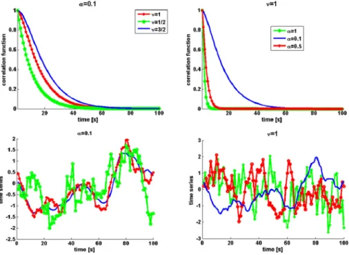
From Eq. (8), the behaviour of Sð Þx by letting x!0 is both influenced by the smoothnessmand the correlation parametera. For high frequencies, i.e.x! 1, the role ofmis more important. Figure1shows for different parameter sets½a;mthe corresponding covariance function (top) and its realization (bottom). The time series are simulated thanks to an eigenvalue decomposition of the Toeplitz covariance matrix built using Eq. (7).
Smooth time series are corresponding to highm(Fig.1left). A visual determination of the smoothness of the corresponding time series is difficult to assess from the correlation function itself. On the other hand,ais related to the correlation length as highlighted in Fig.1(right), i.e. asaincreases, the correlation length decreases.
The Ma´tern parameters can be estimated from the data via Maximum Likelihood Estimation (Handcock and Wallis1994), or fixed aprori (Stein1999) which was implicitly done by Howind et al. (1999), El-Rabbany (1994) when using an exponential function to model carrier phase correlations of GPS observations. Indeed, particular cases corre- sponding to a smoothness of 1=2;1;1are known in geodesy as the exponential covariance function, the first order Markov or the Gaussian model respectively (Whittle1954; Gra- farend and Awange2012; Meier1981). Other parametrizations of the Ma´tern covariance function presented in Eq. (7) exist as well as covariance functions that model hole effects or small negative correlations based on exponentially damped cosine functions (Zastavnyi 1993). Such functions will not be used here as the correlation length and smoothness are
Fig. 1 Example of Ma´tern covariance functions by varying the parameter set ½a;m. Top: correlation function fora¼0:1 by varyingm(left) and correlation function form¼1 by varyinga(right). Bottom:
corresponding time series
more important parameters than trying to take small cosine variations in consideration that may not be physically plausible. A simple, realistic and easy to use modelling of the correlations is our goal, the corresponding covariance matrices being further processed in weighted least-squares adjustments.
3 A model for correlations of GPS phase observations 3.1 Introduction
The proposed function is based on the Ma´tern covariance family and is directly inspired from Wheelon (2001) and Kermarrec and Scho¨n (2014) who derived a function for cor- relations between satellite measurements due to turbulent fluctuations of the index of refractivity. It can be seen as an extension of this model to other kind of elevation dependent correlation factors. We note moreover that Luo (2012) showed that the corre- lation structure of pre-processed residuals from GPS positioning adjustment can be modelled thanks to AR or ARIMA processes. Although not exactly corresponding (Ras- mussen and Williams2006), the underlying differential equations of ARIMA and Ma´tern processes exhibits similarities as the spectral densities are for both cases rational and polynomial. Exemplarily, the AR(2) model can be expressed with a Ma´tern covariance function.
3.2 Proposal for modelling phase correlations
The proposed covariance functionCbetween 2 observations of satellitesiandjat timet andtþsreads:
Citjtþs¼ qd
sinðElið Þt ÞsinEljðtþsÞð Þas mKmð Þas ð9Þ where Eli andElj are the elevations of the satellitei and j respectively. d is a scaling parameter so that the variance equals 1 for satellites at 90elevation using small argument approximations (Scho¨n and Brunner 2008). q is a weighting factor which models the covariance between different satellites. We take hereq¼1 fori=jandq¼0:1 else, see Kermarrec and Scho¨n2014,2017for more details. A possible effect of underestimatingq fori=jin LS adjustments was shown to be a smaller aposteriori variance factor with respect to the apriori value.
This covariance function is derived from a spectral density function and remains therefore positive definite as long as the elevation is not 0.
The variance of our model is based on the commonly used 1
sin2ð ÞEl function. In order to account for non-stationarity of the covariance (i.e. spatiotemporal dependency), a weighting factor 1
sinðElið Þt ÞsinEljðtþsÞ is used to compute inter-satellites correla- tions. This factor is derived from GPS path signals through the atmosphere (Wheelon 2001).
3.3 Building fully populated VCM
Apriori fully populated covariance matrices accounting for correlations of one satellite with itself or with other one at one station can be built thanks to Eq. (9). The resulting cofactor matrix for station A as defined in Eq. (5) is given by:
W^A¼
C1;1A C1;2A C1;3A C1;sA C2;2A C2;3A C2;sA
C3;3A
Cs;sA 2
66 64
3 77
75 ð10Þ
where the subscript A stays for station A and the matricesCi;jA are computed thanks to Eq. (9).
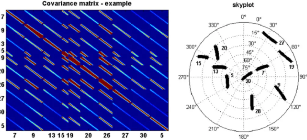
For a better visualization, Fig.2(left) presents an example of the obtained structure of the resulting fully populated covariance matrices sorted per PRN. It corresponds to a standard GPS constellation (Fig.2right) with 10 satellites, one batch having 100 obser- vations and a data rate of 30 s. Depending on the processing strategy of the observations, double differenced matrices should be formed following Eq. (5).
3.4 Estimating the parameters of the covariance function from the observations
Usually, the parameters½a;mare estimated by Maximum Likelihood (Stein1999). Due to the complexity of the fully populated VCM for GPS observations, we propose two ways of estimating½a;m
• Estimation of one set of parameters½a;mfor each satellite by MLE for a batch of 1 h of observations. This set is kept and has an estimated validity of 4–6 h depending on the variations of atmospheric conditions and satellite geometry.
Fig. 2 An example of a fully populated covariance matrix computed with the proposed model (left). The matrix is composed of different non Toeplitz block matrices sorted per satellites. The block diagonal VCM corresponds to the temporal correlations for one satellite with itself whereas the submatrices describe the correlations between one satellite and all other ones. For this example we used½a;m ¼½0:01;1. The last block matrix is corresponding to the VCM of the reference satellite PRN5. The corresponding sky distribution is presented on the right
• An alternative and less computation demanding procedure is only based on the computation of the Ma´tern parameters by MLE for the satellite of reference. The corresponding values found were shown to be closer to a diagonal model (i.e. lower correlation length) than the previous solution and thusacan be decreased by 0.005 s-1 to account for this effect.
As we empirically found that values ofm[2 may lead to some computational problems, we propose not to allow the estimated smoothness parameter to be greater than 3/2. Due to the non-orthogonality of the Ma´tern parameters, this is similar to taking a smallera, i.e. a longer correlation length.
For medium and long baselines, the double differenced observations may contain unmodelled effects. Thus, instead of computing the correlation structure based on the observations at one station, we suggest to directly estimate½a;mfrom the double differ- enced observations.
In order to account for additive noise, a more general form of the covariance matrix for a station A can be used, i.e.W^0¼anoiseW^Aþð1anoiseÞW^noise;withanoise having to be estimated with½a;mby MLE. For elevation dependent noise,W^noise¼W^ELEV;A(called the ELEV matrix) represents the elevation dependent diagonal covariance matrix corre- sponding to a 1
sin2ð ÞEl variance model. Depending on the noise structure that one wish to modelW^noisecan also be replaced by the identity matrix. Intuitively, adding noise matrices will act on stabilizing the fully populated covariance matrices, similarly to a Tikhonov regularization (Tikhonov et al. 1995). It also impact the least-squares results, i.e. they become closer to the one given if only the corresponding diagonal VCM would have been used (Kermarrec and Scho¨n2017). Due to the non-orthogonality of the Ma´tern parameters (Gelfand et al. 2010), estimating a noise matrix will moreover lead in a shift of the corresponding set. Thus, if noise is wrongly taken into account, it will result in a smaller correlation length with noise matrix by same smoothness.
3.5 Comments on the proposed model
Our model is flexible and accounts for many factors (non-stationarity, elevation depen- dency, smoothness, correlation length), modelling implicitly many causes of correlations without expressing them individually. However, as every model, it remains a simplification of the correct but unknown correlation structure. It may be pointed out that also with LS- VCE procedures, simplifications are often necessary to have positive definite VCM by assuming for instance Toeplitz covariance matrices. In order to assess how the Ma´tern parameters influence the least-squares results, interested readers can consult the results of a sensitivity analysis based on simulations and two case studies for long and short baselines in Kermarrec and Scho¨n (2017).
In the next section, we will focus on the effect of this new model both at the obser- vations level and on some least-squares quantities such as the cofactor matrix of the estimates (Eq.3) corresponding to the error ellipsoid, the aposteriori variance factor (Eq.4) and the estimates (Eq.2). A real positioning scenario is studied, the true covariance matrix of the observations being from now unknown.
4 Using the correlation model in a least-squares adjustment: a case study 4.1 Description of the data set
GPS L1 data from the European Permanent Network EPN (Bruyninx et al.2012) from two stations KRAW and ZYWI are chosen as example for a medium baseline (80 km) posi- tioning scenario. The observations have a 30 s rate, a cutoff of 3was applied. The North East Up (NEU) coordinates are computed with double differences for 20 consecutive batches starting at GPS day DOY220, GPS-SOD 6000 s. Each batch represents 100 epochs (i.e. 3000 s). This number of epochs was chosen for two reasons. Firstly, it ensures that the correlation reaches the 0-value inside the batch so that the inversion of the VCM is accurate. Secondly, the correlation structure of small batches of observations is more difficult to assess and the values found may vary more strongly from batch to batch.
The ambiguities are solved in advance thanks to the Lambda method. The results of the case study are not impacted by the integer fixing method. Please note that they are not comparable with those found in Kermarrec and Scho¨n (2017) for the same baseline, the methodology being different (i.e. same design matrix, different days).
The reference values for the station coordinates are the long term values from the EPN solution. The ionosphere-free linear combination L3 was additionally computed. The data were not sophistically filtered (i.e. for instance against multipath effects) in order to keep low frequencies variations in the measurements to study the whitening potential of our fully populated VCM. Because the batch length is shorter than 1 h, no tropospheric parameter was estimated. Nevertheless, estimating this parameter additionally was shown not to influence strongly the conclusions of our case study.
A realistic apriori variance factorr0for double differenced observations of 4 mm was taken into account. A critical value of 4.7 mm corresponding to the Central F-distribution withp=0.1 was chosen for the overall model test (Teunissen2000). We assume that the GPS phase observations are normally distributed (Luo et al.2011).
The correct covariance structure of the observations is unknown and computed fol- lowing the methodology presented in Sect.3. The results from three stochastic models are compared: the ID model corresponding to an identity VCM, the ELEV model where correlations are disregarded and the variance corresponds to a 1
sin2ð ÞEl variance model and the proposed correlation model with different parameter sets½a;m. This strategy aims to study the impact of a misspecification of the stochastic model.
The following quantities are analysed:Eð Þ, i.e. the mean of the aposteriori variance ofr^0
unit weight over all mbatches, the mean of the 3Drms of the estimates defined for one batch as 3Drms¼
ffiffiffiffiffiffiffiffiffiffiffiffiffiffiffiffi
traceðx^Tx^Þ
3
q
. The behaviour ofQx^c andr^0Qx^c are added exemplarily for one batch.
As the variations of½a;mfor the 20 batches of interest were below½0:005;0:1leading to negligible variations of the estimated parameters following Kermarrec and Scho¨n (2017), the correlation structure estimated by MLE was fixed to½a;m0¼½0:012;1:1for the entire time span. The noise factor was set to 0, making use of the non-orthogonality of the Ma´tern parameters (Gelfand et al.2010).
4.2 Impact on the observations
When taking correlation into account in the least-squares adjustment, the effect on the whitening of the residuals is an important criterion (Wang et al.2002).
The fully populated matrices obtained with our model can be shown to be able to whiten the double differenced GPS observations better than the corresponding diagonal matrices, particularly in the low frequency domain. We define a whitened time series lwhite as lwhite¼W^1=2
lwherelis the original time series.W^ is the estimated double differenced VCM corresponding to the ID, ELEV or correlation models.
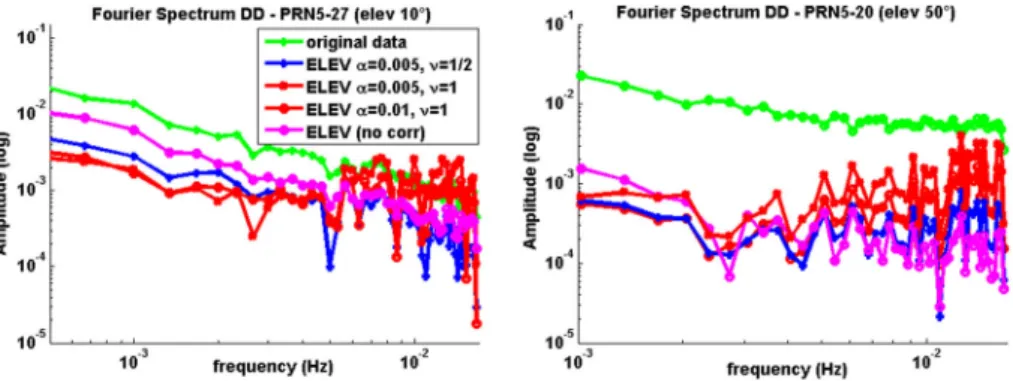
In order to have an insight on how VCM act on correlated observations, the amplitude Fourier spectra of two whitened Double Differenced time series are presented in Fig.3.
The case study from the last section (Fig.2) is carried out. Figure3(left) corresponds to double differences using a low elevation satellite (10elevation) whereas Fig.3(right) is using a satellite at 50elevation. Both were observed during 200 epochs which corresponds to approximately 2 h of observations. Due to the elevation dependency of our model, the whitened double differenced time series are studentized (Luo2012) allowing comparisons between ELEV and correlation models. Thus, the decomposition of the original—non studentized-time series is only given exemplarily. An exact explanation of why particular frequencies are present or not (i.e. multipath, site specific effects) is here on purpose not proposed.
4.2.1 Impact of the smoothnessm
From Fig.3, the impact of the smoothness factormon the whitening can be seen, i.e. the noise at high frequencies is strongly increased with fully populated VCM with respect to the ELEV model (pink line). A VCM with a smoothness of corresponding to an exponential correlation model with an elevation dependent variance is less able to whiten the time series than when a smoothness of 1 is considered (blue versus red lines). This result is coherent with the values found by MLE (Sect.4.1) and particularly visible for the low elevation satellite (Fig.3 left). Indeed, for the same a¼0:005, a more efficient
Fig. 3 Fourier decompositions of different whitened double differenced observations versus log-frequency (Hz). (Left) corresponds to a satellite starting at 10elevation and (right) at 50elevation. The amplitude is
filtering of the low frequencies is obtained withm¼1 (red line) than with m¼1=2 (blue line).
4.2.2 Impact of the correlation parametera
Following Eq. (8), the parameteraplays a more important role at low frequencies. This becomes evident in Fig.3(right) by comparing the two red lines (a¼0:005 anda¼0:01) corresponding to a common smoothness of 1. However, the smoothness still impacts the frequency content of the whitened time series at low frequencies [see Fig.3(left), blue and red lines].
Compared with the whitening obtained with the ELEV model, it can be concluded that the fully populated VCM act both on filtering the low frequencies and increasing the high frequencies content. A lower smoothness ofis suboptimal for both cases. Adding a noise matrix to the VCM (not shown) would have given a higher amplitude for the low fre- quencies part of the spectrum, following the results given with the ELEV model.
This case study is an example. However, other batches of observations with different lengths and geometries were computed without changing the previous conclusions on the effect of½a;m. An exact white noise time series should not be expected and will never be obtained as the apriori VCM are not corresponding exactly to the true VCM of the observations.
4.3 Impact on the least-squares results 4.3.1 Cofactor matrix of the estimates
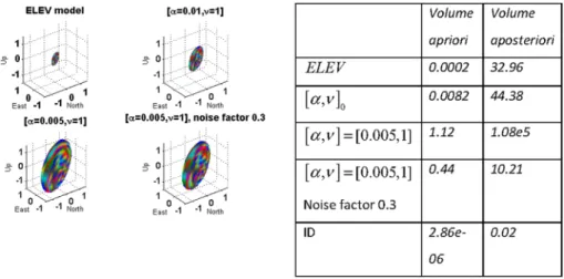
In this section, the impact of the fully populated covariance matrices of the observations on the cofactor matrix of the estimates is considered. One batch corresponding to a standard geometry is taken as example. In Fig.4(left), the 3D apriori error ellipsoids are plotted for different covariance matrices. The corresponding volumes are given in Fig.4(right) forQx^
andr^2Qx^.
Fig. 4 Impact of varying the VCM on the Point error ellipsoid of the estimate (left) and (right) on the volume of the corresponding apriori and aposteriori ellipsoids
From Fig.4(right) and (left) the well-known underestimation of the apriori precision using diagonal VCM is highlighted, the volume of the ellipsoid being up to 40 times smaller than for the fully populated case with½a;m0. Using a lowa¼0:005 leads to an overestimation of the precision with a volume 100 times higher than for½a;m0. This effect is related to the inverse of the covariance matrices and can be easily proven if an AR(1) process is considered (Appendix, see also Rao and Toutenburg1999). It is thus important when using apriori VCM to control the validity of the solution by using exemplarily an overall model test.
We note that the volume of the apriori ellipsoid can be artificially decreased by adding a noise matrix [Fig.4(left) right bottom] by a factor two compared with½a;m ¼ ½0:005;1, no noise. Thus the non-unicity of the parameters is highlighted as different sets may lead to the same results for this quantity. This effect does not mean that one set should not be preferred as mentioned in Sect.4.2, the whitening of the observations being strongly impacted by½a;mas well as the noise factor. The orientations in space of all the ellipsoids are similar by\1as long as the same cosine variance model is used. Taking an identity model changes the orientation of the axis. However, the volume of the error ellipsoid is underestimated by more than a factor 1000 in both apriori and aposteriori case.
From Fig.4(right), the aposteriori ellipsoid with the ELEV model seems to be a better estimation of the precision and nearly corresponding to the reference value of 44.38.
However, this higher volume has to be linked with a higher r^(Sect.4.4) and the corre- sponding solution should be excluded with an overall model test. Thus the least-squares results should always be critically considered to avoid a model misspecification and generally if correlations are present, they should not be neglected for coherence and reliability of the solution.
4.3.2 Impact on the aposteriori variance factor and the estimates
A poorly estimated apriori VCM leads to a biased least-squares solution. The biases of the aposteriori variance factor and the estimates can be expressed literally, see Xu (2013) and Kutterer (1999). However, these formulas necessitate the knowledge of the true VCM and are essentially useful for simulations purpose (Kermarrec and Scho¨n2017). In real case, the global validity of the solution can be checked thanks to the overall model test. In our case moreover, the true coordinates are known. Thus, we consider that the more accurate solution corresponds to the smallest 3Drms.
Following the methodology of 3.3.1., Table1 presents the results obtained by using different Ma´tern parameter sets.
The first line of Table1highlights the effect of a smalla(i.e. a too long correlation length). It can be seen that both the 3Drms and the aposteriori variance factor will be impacted by such a misspecification. For instance, the 3Drms increases from 35% with
a;m
½ ¼ ½0:001;1compared with the reference set. At the same time,Er^W^
is over the apriori value decreasing the number of batches available for computing the solution. Thus, we point out the importance of avoiding an underestimation of the parametera as men- tioned in 3.3.1. The effect of increasingais not presented for sake of shortness. It leads however to a solution which becomes closer to the one given with the ELEV model.
In the second line of Table1, the smoothness is decreased to corresponding to an exponential model. A negligible increase of the 3Drms can be seen whena¼a by at the
similar with the one of½a;m0, pointing out the non-unicity of the best solution. Thus, the effect of taking a smoothness of can be compensated by decreasing a. We highlight however that the whitening of the observations will not be similar, particularly at high frequencies (Sect.4.1).
If the correlations are disregarded, we note a strong increase ofE r^^
W
to 9.5 mm with the ELEV model and 22 mm using the ID model. Thus without adapting the apriori variance factor, no solution could be computed. However, if we increase artificiallyr0to reach theE r^^
W
, the 3Drms with the ELEV model gets similar to the value found with fully populated VCM. This solution remains statistically incorrect and fully populated models should be preferred due to the realistic E r^^
W
. For the ID model, a model misspecification can be guessed asE r^^
W
reaches 22 mm and the 3Drms is 27 mm over the ELEV value.
4.4 L3 dataset and short baselines
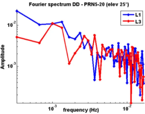
In order to assess to which extend fully populated VCM would impact observations from the ionosphere-free linear combination, the Fourier amplitude spectrum of the double differenced time series with a satellite at 25 elevation is analysed in Fig.5. L1 mea- surements exhibit stronger low frequency between 0.0005 and 0.004 Hz than L3 obser- vations (i.e. between 2 and 10 times higher for L1 than for L3) due to the remaining unmodelled ionospheric effects. The high frequencies content is however similar for L1 and L3.
Consecutively, the impact of fully populated VCM on the whitening of L3 observations will be less important as a ML estimation of½a;m ½0:028;1highlights. Due to the low correlation level, the effect on the least-squares results will not be as important as for L1 observations. Indeed, using the same data set and methodology as previously, the apos- teriori variance factor was found to be 2.8 mm for the fully populated case and 3.3 mm for the ELEV case. Correspondingly, the 3Drms showed an improvement at the submm level:
from 2.17 mm with the diagonal to 2.15 mm with the correlation model.
Table 1 E r^^
W
and the mean of the 3Drms are computed with VCM corresponding to different parameter sets½a;m. The results obtained for diagonal VCM (ELEV and ID) are given additionally. An overall model test was applied
a;m
½ 0¼½0:012;1:1 ½a;m ¼ ½0:005;1 ½a;m ¼ ½0:001;1
Eð3DrmsÞ[mm] 55.95 63.42 75.00
Er^W^
[mm] 3.43 3.91 4.52
a;m
½ ¼ ½0:01;1=2 ½a;m ¼ ½0:005;1=2 ELEV ID
Eð3DrmsÞ[mm] 56.07 55.90 57.07(adaptedr0) 82.71(adaptedr0) Er^W^
[mm] 3.79 3.38 9.73 22.79
Bold corresponds to the Matern parameter set found by MLE whereas italic means that anadaptedr0was used to compute the solution
These variations can be considered as negligible. Thus, the filtering effect of fully populated VCM is less important than for the corresponding L1 observations. Results with short baselines are similar, the frequency content being, expect in extreme cases when for instance multipath is present, homogeneous and close to a white noise. However, this does not mean that correlations should be neglected. In case of multipath, the more realistic aposteriori variance factor obtained with fully populated VCM can influence positively the 3Drms when the overall model test is applied, particularly when batches of less than 1 h are computed.
5 Conclusions: on taking correlations into account
Because it remains easier to use diagonal covariance matrices in a least-squares adjustment for relative positioning, correlations of GPS phase observations are generally neglected. In this contribution, an innovative model based on the flexible and easy to use Ma´tern covariance family adapted to GPS observations was presented. Both the smoothness and the correlation length are allowed to vary in a physically plausible range. These parameters are determined by MLE either for all satellites independently or only for the reference satellite. Fully populated variance covariance matrices can be built and integrated in the least-squares adjustment.
Thanks to a particular case study corresponding to a 80 km long baseline, the model was shown to give a better whitening of the observations. If the smoothness impacts more strongly the high frequency content, the correlation parameter allows a down weighting of the low frequencies that come from unmodelled effects. Moreover, a more realistic pre- cision together with reliable results from test statistics such as the overall model test could be obtained, the impact at the estimates level being negligible compared with results found with the cosine variance model that disregards correlations. The risks of underestimating the correlation parameter were pointed out as leading to a higher aposteriori variance factor and voluminous error ellipsoid, whereas a low smoothness gave results close to the diagonal model.
Thanks to the parametric formulation, the proposed model can be adapted to various
Fig. 5 Fourier amplitude spectrum for L1 and L3 double differenced observations. A satellite at 25elevation was chosen
exponential model is comparable as long as the correlation parameter is decreased accordingly by approximately 0.005. In that case, the VCM becomes invertible thanks to a close formula. As a consequence, the equivalent diagonal model proposed by Kermarrec and Scho¨n (2016) can be easily use, allowing more reliable least-squares results by less computational burden.
Acknowledgements The authors gratefully acknowledge the EPN network and corresponding agencies for providing freely the data. Anonymous reviewers are warmly thanks for their valuable comments which helped improve the original manuscript.
Appendix: On the inverse of the covariance matrix
Studying the inverse of the fully populated covariance matrix is interesting to gain a better insight on the way correlations act on the previous results, particularly on the apriori cofactor matrix of the estimates and by extension of the ambiguities.
However, except in particular cases, VCM based on Ma´tern model do not have an explicit formulation of their inverse. We will therefore first present the particular case of an AR(1) process and in a second step take an example of the matrices used in this article.
AR(1) and Ma´tern matrices
In this case, the inverse of the covariance matrix reads
W1ARð1Þ¼ 1 1q2
1 q 0 . . . 0 0
q 1þq2 q .. .
0 0
0 q 1þq2 .. .
0 0
... .. .
.. . .. .
.. . 0
0 0 0 .. .
1þq2 q
0 0 0 . . . q 1
2 66 66 66 66 64
3 77 77 77 77 75
whereqis the autocorrelation function.
Thus, from a fully populatedWARð1Þ, only a sparse matrix remains which lines have 2 different values (1) the diagonal elements and (2) a negative value on the off-diagonal. A scaling factor 1q12 depending on the correlation length can be further identified. This structure can be extended for Ma´tern covariance matrices, i.e. a factor depending on the Ma´tern parameter set chosen is mainly responsible for the scaling of apriori cofactor matrices of the estimates as shown in Sect.4. The error ellipsoid may thus be artificially too voluminous if a wrong correlation structure is taken into account.
Taking noise matrix into account
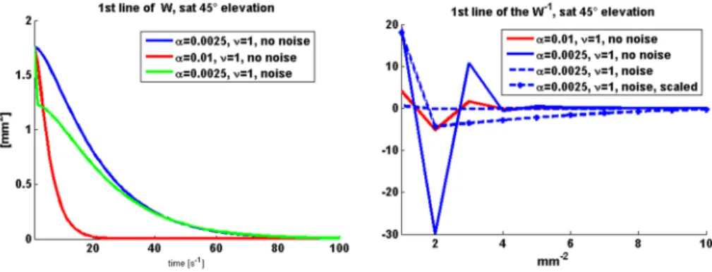
In order to see how noise matrices are impacting the inverse of the covariance matrices, a particular case is chosen to compute the covariance function as defined in Eq. (9) corre- sponding to a satellite at 45elevation. Only the first 100 epochs of the block diagonal matrix are analysed.
Fig.6 (left) shows the corresponding line of the covariance matrix for different cor- relation structures. For½a;m ¼ ½0:0025;1and due to the smoothness of 1, the first values of the covariance decreases slowly with time
The corresponding line of the inverse of the covariance matrix for the different cases are depicted in Fig.6(right). The signature of the inverse of a fully populated VCM is clearly seen when no noise matrix is taken in consideration, i.e. small oscillations around the 0–
value. The amplitude of the variations increases asadecreases. If a noise matrix is added only the first oscillation remains, the other ones being replaced by a ramp, thus damping the effect of the correlations. This was highlighted by studying the whitening of the residuals and this is the reason why the results given with or without noise matrix are similar up to a given value ofaandmwhere the equivalence between the smoothed and the original curve is getting too high.
References
Abramowitz M, Segun IA (1972) Handbook of mathematical functions. Dover, New York
Amiri-Simkooei AR, Teunissen PJG, Tiberius C (2009) Application of least-squares variance component estimation to GPS observables. J Surv Eng 135(4):149–160
Amiri-Simkooei AR, Jazaeri S, Zangeneh-Nejad F, Asgari J (2016) Role of stochastic model on GPS integer ambiguity resolution success rate. GPS Solut 20(1):51–61
Bischoff W, Heck B, Howind J, Teusch A (2005) A procedure for testing the assumption of homoscedasticity in least squares residuals: a case study of GPS carrier-phase observations. J Geodesy 78(2005):379–404
Bona P (2000) Precision, cross correlation, and time correlation of GPS phase and code observations. GPS Solut 4(2):3–13
Bruyninx C, Habrich H, So¨hne W, Kenyeres A, Stangl G, Vo¨lksen C (2012) Enhancement of the EUREF permanent network services and products. Geodesy Planet Earth IAG Symp Ser 136:27–35 El-Rabbany A (1994) The effect of physical correlations on the ambiguity resolution and accuracy esti-
mation in GPS differential positioning. Ph.D. thesis, Department of Geodesy and Geomatics Engi- neering, University of New Brunswick, Canada
Gelfand AR, Diggle PJ, Fuentes M, Guttorp P (2010) Handbook of spatial statistics. Chapman & Hall/CRC Handbooks of Modern Statistical Methods, London
Grafarend EW, Awange J (2012) Applications of linear and nonlinear models. Springer, Berlin Greene WH (2003) Econometric analysis, 5th edn. Prentice Hall, Upper Saddle River
Fig. 6 Left: exemplarily line of the non-double differenced VCM for different parameter sets with and without a noise VCM and right the corresponding inverse. The satellite taken is having a 45elevation
Howind J, Kutterer H, Heck B (1999) Impact of temporal correlations on GPS-derived relative point positions. J Geodesy 73(5):246–258
Jin SG, Luo O, Ren C (2010) Effects of physical correlations on long-distance GPS positioning and zenith tropospheric delay estimates. Adv Space Res 46:190–195
Journel AG, Huifbregts CJ (1978) Mining geostatistics. Academic Press, New York
Kermarrec G, Scho¨n S (2014) On the Ma´tern covariance family: a proposal for modeling temporal corre- lations based on turbulence theory. J Geodesy 88(11):1061–1079
Kermarrec G, Scho¨n S (2016) Taking correlations into account with a diagonal covariance matrix.
J Geodesy 90(9):793–805
Kermarrec G, Scho¨n S (2017) Apriori fully populated covariance matrices in least-squares adjustment—case study: GPS relative positioning. J Geodesy 91(5):465–484
Koch KR (1999) Parameter estimation and hypothesis testing in linear models. Springer, Berlin Kutterer H (1999) On the sensitivity of the results of least-squares adjustments concerning the stochastic
model. J Geodesy 73:350–361
Leandro R, Santos M, Cove K (2005) An empirical approach for the estimation of GPS covariance matrix of observations. In: proceeding ION 61st annual meeting, The MITRE Corporation & Draper Laboratory, 27–29 June 2005. Cambridge
Li B (2016) Stochastic modeling of triple-frequency BeiDou signals: estimation, assessment and impact analysis. J Geodesy 90(7):593–610
Li B, Shen Y, Lou L (2008) Assessment of stochastic models for GPS measurements with different types of receivers. Chin Sci Bull 53(20):3219–3225
Li B, Lou L, Shen Y (2016) GNSS elevation-dependent stochastic modelling and its impacts on the statistic testing. J Surv Eng 142(2):04015012
Luo X (2012) Extending the GPS stochastic model y means of signal quality measures and ARMA pro- cesses. Ph.d. Karlsruhe Institute of Technology
Luo X, Mayer M, Heck B (2011) On the probability distribution of GNSS carrier phase observations GPS Solution 15(4):369–379
Ma´tern B (1960) Spatial variation-Stochastic models and their application to some problems in forest surveys and other sampling investigation. PhD Meddelanden Fra˚n Statens Skogsforskningsinstitut Band 49, Nr 5
Meier S (1981) Planar geodetic covariance functions. Rev Geophys Space Phys 19(4):673–686
Misra P, Enge P (2012) Global positioning system. Revised Second Edition, Ganga-Jamuna Press, Lincoln, Massachusetts
Moschas F, Stiros S (2013) Noise characteristics of high-frequency, short-duration GPS records from analysis of identical, collocated instruments. Measurement 46(2013):1488–1506
Radovanovic RS (2001) Variance-covariance modeling of carrier phase errors for rigorous adjustment of local area networks. In: IAG 2001 scientific assembly. Budapest, Sep 2–7, 2001
Rao C, Toutenburg H (1999) Linear models, least-squares and alternatives. Springer, New York Rasmussen CE, Williams C (2006) Gaussian processes for machine learning. MIT Press, Cambridge Santos MC, Vanicek P, Langley RB (1997) Effect of mathematical correlation on GPS network compu-
tation. J Surv Eng 123(3):101–112
Satirapod C, Wang J, Rizos C (2003) Comparing different GPS data processing techniques for modelling residual systematic errors. J Surv Eng 129(4):129–135
Scho¨n S, Brunner FK (2008) A proposal for modeling physical correlations of GPS phase observations.
J Geodesy 82(10):601–612
Seeber G (2003) Satellite geodesy. Walter de Gruyter, Berlin
Stein ML (1999) Interpolation of spatial data. Some theory for kriging. Springer, New York
Teunissen PJG (2000) Testing theory and introduction. Series on Mathematical Geodesy and Positioning.
Delft University Press, Dordrecht
Teunissen PJG, Amiri-Simkooei AR (2008) Least-squares variance component estimation. J Geodesy 2008(82):65–82
Tiberius C, Kenselaar F (2000) Estimation of the stochastic model for GPS code and phase observables.
Surv Rev 35(277):441–454
Tikhonov AN, Goncharsky AV, Stepanov VV, Yagola AG (1995) Numerical methods for the solution of Ill- posed problems. Kluwer Academic Publishers, Dordrecht
Wang J, Satirapod C, Rizos C (2002) Stochastic assessment of GPS carrier phase measurements for precise static relative positioning. J Geodesy 76(2):95–104
Wheelon AD (2001) Electromagnetic scintillation part I GeomETRICAL OPTICS. Cambridge University Press, Cambridge
Whittle P (1954) On stationary processes in the plane. Biometrika 41:434–449
Wild U, Beutler G, Gurtner W, Rothacher M (1989) Estimating the ionosphere using one or more dual frequency GPS receivers. In: Proceedings of the 5th international geodetic symposium on satellite positioning. Las Cruces, pp 724–736
Xu P (2013) The effect of incorrect weights on estimating the variance of unit weigth. Stud Geophys Geodesy 57:339–352
Yaglom AM (1987) Correlation theory of stationary and related random functions I basic results. Springer, New York
Zastavnyi VP (1993) Positive definite functions depending on a norm. Russ Acad Sci Doklady Math 46:112–114