Ranking in Swiss system chess team tournaments
by László Csató
C O R VI N U S E C O N O M IC S W O R K IN G P A PE R S
http://unipub.lib.uni-corvinus.hu/1830
CEWP 1 /201 5
Ranking in Swiss system chess team tournaments
L´ aszl´ o Csat´ o
*Department of Operations Research and Actuarial Sciences Corvinus University of Budapest
MTA-BCE ”Lend¨ulet” Strategic Interactions Research Group Budapest, Hungary
January 8, 2015
Abstract
The paper uses paired comparison-based scoring procedures for ranking the participants of a Swiss system chess team tournament. We present the main challenges of ranking in Swiss system, the features of individual and team competitions as well as the failures of official lexicographical orders. The tournament is represented as a ranking problem, our model is discussed with respect to the properties of the score, generalized row sum and least squares methods. The proposed procedure is illustrated with a detailed analysis of the two recent chess team European championships. Final rankings are compared by their distances and visualized with multidimensional scaling (MDS). Differences to official ranking are revealed by the decomposition of least squares method. Rankings are evaluated by prediction accuracy, retrodictive performance, and stability. The paper argues for the use of least squares method with a results matrix favoring match points.
JEL classification number: D71
Keywords: Paired comparison, ranking, least squares method, Swiss system, chess
* e-mail: laszlo.csato@uni-corvinus.hu
1 Introduction
Sport is a classical field of paired comparison-based ranking, early works were often inspired by chess tournaments (Landau, 1895, 1914; Zermelo, 1929). In the paper we deal with ranking in Swiss system chess team tournaments. This issue were partly discussed by Csat´o (2013), here a deeper methodological foundation will be given for the problem and the evaluation of rankings will be revisited. However, we do not discuss the issue of pairing in Swiss system tournaments.
The paper considers a parametric family of scoring methods, the generalized row sum (Chebotarev, 1989, 1994) as well as the least squares method. We do not know any application of the former procedure, while the latter was extensively used for sport rankings (Leeflang and van Praag, 1971; Stefani, 1980). Our analysis is based on some recent results: Gonz´alez-D´ıaz et al. (2014) have presented the axiomatic properties of generalized row sum and least squares, Csat´o (2014a) has given an interpretation for the least squares method, and Can (2014) has contributed to the choice of distance functions between rankings. Brozos-V´azquez et al. (2010) argues for the use of recursive methods as a tie-breaking rule in Swiss system chess tournaments.
The paper is structured as follows. Section 2 shortly outlines the ranking problem, ranking methods and their relevant properties. Section 3 aims to incorporate Swiss system chess team tournaments into this framework. We present the main challenges of ranking in these type of tournaments, the features of individual and team competitions as well as the failures of official lexicographical orders.
The proposed model is applied in Section 4 to ranking the participants in the 2011 and 2013 European Team Chess Championship open tournaments. We introduce twelve rankings distinguished by the role of opponents and match versus table points. Rankings are compared on the basis of their distances and visualized with multidimensional scaling (MDS). Differences to official ranking are revealed by the decomposition of least squares
method.
On the basis of these examples, we argue for the use of least squares method with a generalized result matrix favoring match points. The proposal is based on a lot of findings, variance with respect to the chosen results matrix as well as prediction accuracy, retrodictive performance (the ability to match the outcomes of matches already played) and robustness (stability of the ranking between two subsequent rounds).
Finally, Section 5 summarize our findings and review possible extensions of the model.
Some results of the calculations are detailed in the Appendix. A reader familiar with ranking problems (Gonz´alez-D´ıaz et al., 2014; Csat´o, 2014a) may skip Section 2, and knowledge on Swiss system chess tournaments may save from the study of Subsection 3.1.
Most results mentioned above are our contribution. We do not know any formal discussion of ranking in Swiss system tournaments (suggestions by Brozos-V´azquez et al.
(2010) are more or less based on intuition) together with investigations through examples, despite the latter was given, for instance, by Jeremic and Radojicic (2010), Csat´o (2012), and Csat´o (2013). MDS has been applied first for the comparison of rankings in Csat´o (2013). According to our knowledge, we are the first to use the weighted distance of Can (2014). Stability is also a new idea in the evaluation of Swiss system tournament rankings.
2 The ranking problem and its solution
In the following a model of paired comparison-based ranking is presented. It is a simpler version of Csat´o (2014a), a detailed derivation can be found there.
2.1 The ranking problem
Let 𝑁 ={1,2, . . . , 𝑛}, 𝑛∈N be a set of objects. The matches matrix 𝑀 = (𝑚𝑖𝑗)∈N𝑛×𝑛 contains the number of comparisons between the objects, and is symmetric (𝑀⊤ =𝑀).1 Diagonal elements 𝑚𝑖𝑖 are supposed to be 0 for all 𝑖 = 1,2, . . . , 𝑛, anyway they will not be used. Let 𝑑𝑖 = ∑︀𝑛𝑗=1𝑚𝑖𝑗 be the total number of comparisons of object 𝑖 and d= max{𝑑𝑖 :𝑖∈𝑁} be the maximal number of comparisons with the other objects. Let 𝑚 = max{𝑚𝑖𝑗 :𝑖, 𝑗 ∈𝑁}.
Theresults matrix 𝑅= (𝑟𝑖𝑗)∈R𝑛×𝑛 contains the outcome of comparisons between the objects, and is skew-symmetric (𝑅⊤ =−𝑅). All elements are limited by𝑟𝑖𝑗 ∈[−𝑚𝑖𝑗, 𝑚𝑖𝑗].
(𝑟𝑖𝑗 +𝑚𝑖𝑗)/(2𝑚𝑖𝑗)∈[0,1] may be regarded as the likelihood that object𝑖 defeats 𝑗. Then 𝑟𝑖𝑗 = 𝑚𝑖𝑗 means that𝑖 is perfectly better than 𝑗, and 𝑟𝑖𝑗 = 0 corresponds to an undefined relation (if 𝑚𝑖𝑗 = 0) or the lack of preference (if 𝑚𝑖𝑗 > 0) between the two objects. A ranking problem is given by the triplet (𝑁, 𝑅, 𝑀). Let ℛ be the class of ranking problems and ℛ𝑛 be the class of ranking problems with|𝑁|=𝑛.
A ranking problem is called round-robin if 𝑚𝑖𝑗 = 1 for all 𝑖̸=𝑗, that is, every object has been compared exactly once with all of the others. A round-robin ranking problem is more general than the binary tournaments of Rubinstein (1980) as it allows for ties (𝑟𝑖𝑗 = 𝑟𝑗𝑖 = 0) and arbitrary preference intensities (𝑟𝑖𝑗 is not necessarily −1 or 1). A ranking problem is called unweighted if 𝑚𝑖𝑗 ∈ {0,1} for all 𝑖 ̸= 𝑗, namely, every paired comparison is carried out at most once. A ranking problem is called balanced if 𝑑𝑖 =𝑑𝑗 for all 𝑖, 𝑗 = 1,2, . . . , 𝑛, that is, every object has the same number of comparisons.
2.2 Ranking methods
Matches matrix 𝑀 can be represented by an undirected multigraph 𝐺:= (𝑉, 𝐸) where vertex set 𝑉 corresponds to the object set 𝑁, and the number of edges between objects 𝑖 and 𝑗 is equal to𝑚𝑖𝑗. The number of edges adjacent to𝑖 is the degree 𝑑𝑖 of node𝑖. A path from object 𝑘1 to object 𝑘𝑡 is a sequence of objects𝑘1, 𝑘2, . . . , 𝑘𝑡 such that 𝑚𝑘ℓ𝑘ℓ+1 >0 for all ℓ= 1,2, . . . , 𝑡−1. Two vertices are connected if 𝐺 contains a path between them. A graph is said to be connected if every pair of vertices is connected.
Graph 𝐺 is called the comparison multigraph associated with the ranking problem (𝑁, 𝑅, 𝑀), and is independent of the results of paired comparisons. The Laplacian matrix 𝐿 = (ℓ𝑖𝑗) ∈ R𝑛×𝑛 of graph 𝐺 is given by ℓ𝑖𝑗 = −𝑚𝑖𝑗 for all 𝑖 ̸= 𝑗 and ℓ𝑖𝑖 = 𝑑𝑖 for all 𝑖= 1,2, . . . , 𝑛.
Vectors are denoted by bold fonts, and assumed to be column vectors. Let e ∈ R𝑛 be given by 𝑒𝑖 = 1 for all 𝑖= 1,2, . . . , 𝑛 and 𝐼 ∈R𝑛×𝑛 be the matrix with 𝐼𝑖𝑗 = 1 for all 𝑖, 𝑗 = 1,2, . . . , 𝑛.
Arating (scoring) method 𝑓 is an ℛ𝑛→R𝑛 function, 𝑓𝑖 =𝑓𝑖(𝑁, 𝑅, 𝑀) is the rating of object𝑖. It defines aranking method by𝑖weakly above𝑗 in the ranking problem (𝑁, 𝑅, 𝑀)
1 In most practical applications (including ours) the condition𝑚𝑖𝑗 ∈Nmeans no restriction. Modifi- cation of the domain toR+ has no impact on the results but the discussion becomes more complicated.
This generalization has some significance for example in the case of forecasting sport results when the latest comparisons give more information about the current form of a player.
if and only if 𝑓𝑖(𝑁, 𝑅, 𝑀)≥ 𝑓𝑗(𝑁, 𝑅, 𝑀). Throughout the paper, the notions of rating and ranking methods will be used analogously since all ranking procedures discussed are based on rating vectors. Rating methods 𝑓1 and 𝑓2 are called equivalent if they result in the same ranking for any ranking problem (𝑁, 𝑅, 𝑀).
Now we introduce some rating methods for a ranking problem (𝑁, 𝑅, 𝑀)∈ ℛ𝑛. Definition 1. Row sum rating method: s:ℛ𝑛→R𝑛 such that s=𝑅e.
Row sum will also be referred to asscores,s is sometimes called the scores vector. It does not take the comparison structure into account.
The following parametric rating procedure was constructed axiomatically by Chebotarev (1989) and thoroughly analyzed in Chebotarev (1994).
Definition 2. Generalized row sum rating method:
x(𝜀) :ℛ𝑛→R𝑛 such that (𝐼+𝜀𝐿)x(𝜀) = (1 +𝜀𝑚𝑛)s, where𝜀 >0 is a parameter.
It follows from the definition that lim𝜀→0x(𝜀) =s. Generalized row sum adjusts the standard scores of objects by accounting for the performance of objects compared with it, and so on. 𝜀 indicates the importance attributed to this correction.
In our model the outcome of paired comparisons is restricted by −𝑚≤𝑟𝑖𝑗 ≤𝑚 for all 𝑖, 𝑗 ∈𝑁. Then we have some results about the choice of 𝜀.
Definition 3. Reasonable choice of𝜀(Chebotarev, 1994, Proposition 5.1): Let (𝑁, 𝑅, 𝑀)∈ ℛ𝑛 be a ranking problem. The value of parameter 𝜀of generalized row sum isreasonable if
0< 𝜀≤ 1 𝑚(𝑛−2). The reasonable upper bound of 𝜀 is 1/[𝑚(𝑛−2)].
𝑛≥3 can be assumed implicitly since the solution becomes trivial for 𝑛 = 2.
Proposition 1. If 𝜀 is reasonable, then −𝑚(𝑛−1)≤𝑥𝑖(𝜀)≤𝑚(𝑛−1)for all 𝑖∈𝑁. Proof. See Chebotarev (1994, Property 13).
Note that −𝑚(𝑛−1) ≤ 𝑥𝑖(𝜀) ≤ 𝑚(𝑛−1) for all 𝑖 ∈ 𝑁 in a round-robin ranking problem (𝑁, 𝑅, 𝑀)∈ ℛ𝑛.
Both the score and the generalized row sum ratings are well-defined and can be obtained from a system of linear equations for all ranking problems.
The subsequent method is well-known in a lot of fields, a review about its origin is given by Gonz´alez-D´ıaz et al. (2014) and Csat´o (2014a).
Definition 4. Least squares rating method: q:ℛ𝑛→R𝑛 such that 𝐿q=s ande⊤q= 0.
It has strong connections to generalized row sum.
Lemma 1. The least squares method is equivalent to the other limit of generalized row sum (𝜀→ ∞), moreover, lim𝜀→∞x(𝜀) = 𝑚𝑛q.
Proof. See Chebotarev and Shamis (1998, p. 326). 𝜀→ ∞ means that expressions with a constant coefficient in the equation system (𝐼+𝜀𝐿)x(𝜀)(𝑁, 𝑅, 𝑀) = (1 +𝜀𝑚𝑛)sbecome negligible.
Proposition 2. The least squares rating q is unique if and only if comparison multigraph 𝐺 is connected.
Proof. In the unweighted case, see Boz´oki et al. (2010, Theorem 4). The same theorem was proved by Kaiser and Serlin (1978, p. 426) in a different way.
The general weighted case is examined in Boz´oki et al. (2014) and Gonz´alez-D´ıaz et al. (2014). Chebotarev and Shamis (1999, p. 220) mention this fact without further discussion.
Proposition 2 causes no problem as in the case of an unconnected comparison multigraph we have independent ranking problems.
A graph-theoretic interpretation of the generalized row sum method is given by Shamis (1994). An iterative decomposition of least squares is provided by Csat´o (2014a).
Proposition 3. Let the comparison multigraph be connected and not regular bipartite.
The unique solution of the least squares problem is q= lim𝑘→∞q(𝑘) where q(0) = (1/d)s,
q(𝑘) =q(𝑘−1)+ 1 d
[︂1
d(d𝐼−𝐿)
]︂𝑘
s (𝑘= 1,2, . . .).
2.3 Some properties of ranking methods
In order to argue for the use of these methods we need to discuss a number of axioms.
Definition 5. Admissible transformation of the results (Csat´o, 2014b): Let (𝑁, 𝑅, 𝑀)∈ ℛ𝑛 be a ranking problem. Anadmissible transformation of the results provides a ranking problem (𝑁, 𝑘𝑅, 𝑀)∈ ℛ𝑛 such that 𝑘 >0, 𝑘 ∈Rand 𝑘𝑎𝑖𝑗 ∈[−𝑚𝑖𝑗, 𝑚𝑖𝑗] for all 𝑖∈𝑁.
Multiplier 𝑘 cannot be too large since −𝑚𝑖𝑗 ≤𝑘𝑟𝑖𝑗 ≤𝑚𝑖𝑗 should be satisfied for all 𝑖∈𝑁 according to the definition of the results matrix. 𝑘≤1 is always allowed.
Definition 6. Scale invariance (𝑆𝐼) (Csat´o, 2014b): Let (𝑁, 𝑅, 𝑀),(𝑁, 𝑘𝑅, 𝑀) ∈ ℛ𝑛 be two ranking problems such that (𝑁, 𝑘𝑅, 𝑀) is obtained from (𝑁, 𝑅, 𝑀) through an admissible transformation of the results. Scoring procedure 𝑓 :ℛ𝑛 →R𝑛 isscale invariant if 𝑓𝑖(𝑁, 𝑅, 𝑀)≥𝑓𝑗(𝑁, 𝑅, 𝑀)⇔𝑓𝑖(𝑁, 𝑘𝑅, 𝑀)≥𝑓𝑗(𝑁, 𝑘𝑅, 𝑀) for all𝑖, 𝑗 ∈𝑁.
Scale invariance implies that the ranking is invariant to a proportional modification of wins (𝑟𝑖𝑗 >0) and losses (𝑟𝑖𝑗 <0). It seems to be important for applications. If the paired comparison outcomes cannot be measured on a continuous scale, it is not trivial how to transform them into 𝑟𝑖𝑗 values. 𝑆𝐼 provides that it is not a problem in several cases. For example, if only three outcomes are possible, the coding (𝑟𝑖𝑗 = 𝜅 for wins; 𝑟𝑖𝑗 = 0 for draws; 𝑟𝑖𝑗 = −𝜅 for losses) makes the ranking independent from 𝜅 > 0. It may also be advantageous when relative intensities are known such as a regular win is two times better than an overtime triumph.
Lemma 2. The score, generalized row sum and least squares methods satisfy 𝑆𝐼.
Proof. See Csat´o (2014b, Lemma 4.3). It is the immediate consequence ofs(𝑁, 𝑘𝑅, 𝑀) = 𝑘s(𝑁, 𝑅, 𝑀).
One disadvantage of the score procedure is that it is independent of irrelevant matches (Gonz´alez-D´ıaz et al., 2014). However, it does not cause problems on the class of round-
robin ranking problems, so it makes sense to preserve the attributes of score on this set.
Definition 7. Score consistency(𝑆𝐶𝐶) (Gonz´alez-D´ıaz et al., 2014): Scoring procedure𝑓 : ℛ𝑛 →R𝑛 is score consistent if 𝑓𝑖(𝑁, 𝑅, 𝑀)≥𝑓𝑗(𝑁, 𝑅, 𝑀)⇔𝑠𝑖(𝑁, 𝑅, 𝑀)≥𝑠𝑗(𝑁, 𝑅, 𝑀) for all 𝑖, 𝑗 ∈𝑁 and round-robin ranking problem (𝑁, 𝑅, 𝑀)∈ ℛ𝑛.
A score consistent method is equivalent to the score in the case of round-robin ranking problems. A similar requirement is mentioned by Zermelo (1929) and David (1987, Property 3).
Remark 1. Regarding the generalized row sum method, Chebotarev (1994, Property 3) introduces a more general axiom called agreement: if (𝑁, 𝑅, 𝑀) ∈ ℛ𝑛 is a round-robin ranking problem, then x(𝜀)(𝑁, 𝑅, 𝑀) =s(𝑁, 𝑅, 𝑀).
Lemma 3. Score, generalized row sum and least squares methods satisfy 𝑆𝐶𝐶.
Proof. For generalized row sum see Remark 1. In the case of least squares the proof is given by Gonz´alez-D´ıaz et al. (2014, Proposition 5.3).
Further properties of the scoring procedures are discussed by Gonz´alez-D´ıaz et al.
(2014) and Csat´o (2014b).
3 Modelling of the problem
Now we are able to discuss ranking in Swiss system chess competitions in the framework presented above.
3.1 Main features of Swiss system chess tournaments
Chess tournaments are often organized in the Swiss system. They go for a predetermined number of rounds, in each round two players compete head-to-head. All of them participate in the entire tournament, none are eliminated. The system is used when there are too many players to play a round-robin tournament consequently there are pairs of players without a match between them. However, it is more efficient than a knock-out tournament as more matches can be played at the same time.
Two emerging issues are how to pair the players and how to rank the participants on the basis of their respective results. The pairing algorithm aims to pair players with a similar performance as measured by the number of their wins and draws (see FIDE (2014) for details). Some proposals have been made to improve them by weighted ( ´Olafsson, 1990) or stable matchings (Kujansuu et al., 1999) but it is out of the scope of this paper.
A match in chess can have three different results: white wins, black wins or draw. The winner gets one point, the loser gets zero points, a draw means half-half points for both players. There are some competitions where a win results in three points and a draw in one point, however, they not fit into our model since then the number of allocated points depends on the result, a win and a loss is not equal to two draws, which violates the skew-symmetricity of the results matrix.
Let us denote the number of rounds by𝑐 and the number of players by 𝑛.
The final ranking of the players is determined by lexicographical orders such that the first rule is the number of points scored. However, it is usually not enough to get a linear order (complete, transitive and antisymmetric binary relation) of the participants: in 𝑐 rounds the number of points is an integer between 0 and 2𝑐so there always will be players with equal score if𝑛 >2𝑐+ 1. Ties are eliminated by the sequential application of various tie-breaking rules (FIDE, 2014).
The difficulties in ranking are caused by different schedules as players with weaker opponents can score the same number of points more easily. A pairing algorithm based on the concept above and lexicographical orders are not able to solve this problem (Csat´o, 2012, 2013; Brozos-V´azquez et al., 2010; Jeremic and Radojicic, 2010). Actually, it prefers players with an improving performance during the tournament contrary to players with a declining one. Take two players 𝑖 and 𝑗 with equal number of points after playing some rounds. Player 𝑖 is said to on theinner circle if it scored more points in the first rounds relative to player 𝑗 who is said to be on the outer circle. Since they have played against opponents with a similar number of points in each round because of the pairing algorithm, it is probable that player 𝑗 has met with weaker opponents. Tie-breaking rules may take the performance of opponents into account but a similar problem may arise if player 𝑗 has a bit more points than player 𝑖 as a lexicographical order is not continuous. Naturally, it is not a precise mathematical argument, although we hope it highlights the main problem with official rankings. It can be argued that an improving performance is better than a declining one, however, it contains a subjective judgment strange to the positive approach of scientific research.
besides individual competitions, there are also team tournaments in chess. They seem to be preferable from a theoretical point of view since in individual championships color allocation has a prominent role, the first-mover with white have an inherent advantage in the game. In team tournaments a match is played on 2𝑡 boards such that𝑡 players of a team play with white and the other 𝑡 players of the team play with black. Therefore it can be accepted that color allocation does not influence the outcome of any matches.
In team championships there is a difference between board points and match points scored. The winner of a game on a board gets 1 board point, the loser 0 points, and the draw yields 0.5 points for both teams, thus 2𝑡 board points are allocated in a given match.
The winner team achieving more (at least𝑡+ 0.5) board points scores 2 match points, the loser 0, while a draw results in 1 match point for both team. Lexicographical orders are usually based on the number of board or match points. Recently the use of match points is preferred as in chess olympiads and team European championships.
Other details on Swiss-system chess team tournaments can be found in Csat´o (2012, 2013).
3.2 Definition as a ranking problem
Paired comparison-based ranking of the objects involves three main challenges. The first one is the possible appearance of circular triads when object 𝑖 is better than object 𝑗 (𝑟𝑖𝑗 > 𝑟𝑗𝑖), object 𝑗 is better than object 𝑘, but object 𝑘 is better than object 𝑖. Circular triads generate difficulties in all paired comparison settings, but, if preference intensities also count, other triplets may cause a problem. The second issue, the varied calibre of the opposition encountered by each object, arises as the consequence of incomplete and multiple comparisons. For example, if object 𝑖 was compared only with object 𝑗, then its rating certainly should depend on the results of object 𝑗. We have seen that this
argument can be continued infinitely. The third problem is the possibly different numbers of comparisons involving the objects, that is,𝑑𝑖 ̸=𝑑𝑗.
According to David (1987), ’it must be realized that there can be no entirely satisfactory way of ranking if the number of replications of each object varies appreciably’. In Swiss system competitions this question does not emerge. The other two will be dealt with the methods presented in Section 2, after any chess team tournament is presented as a ranking problem. Since data are given by sport results, we do not discuss the question whether inherent inconsistency allows to provide a meaningful ranking (Jiang et al., 2011).
Set of objects𝑁 consists of the teams of the competition. Matches matrix 𝑀 is given by 𝑚𝑖𝑗 = 1 if teams𝑖 and 𝑗 have played against each other and𝑚𝑖𝑗 = 0 otherwise. For the sake of simplicity it is assumed that 𝑛 is even, so it is possible that all teams play exactly 𝑐 matches (there are no byes or unplayed matches). First we suggest two extreme possibilities for the choice of results matrix.
Notation 1. 𝑀 𝑃𝑖𝑗 and 𝐵𝑃𝑖𝑗 is the number of match points and board points of team 𝑖 against team 𝑗, respectively.
mp and gp is the vector of match points and board points, respectively.
Rankings derived from mp and bp are the same as the official lexicographical orders based on match points and board points without tie-breaking rules.
Definition 8. Match points based results matrix: Results matrix of ranking problem (𝑁, 𝑅𝑀 𝑃, 𝑀)∈ ℛ𝑛 is based on match points if 𝑟𝑖𝑗𝑀 𝑃 =𝑀 𝑃𝑖𝑗−1 for all 𝑖, 𝑗 ∈𝑁.
Definition 9. Board points based results matrix: Results matrix of ranking problem (𝑁, 𝑅𝐵𝑃, 𝑀)∈ ℛ𝑛 is based on board points if 𝑟𝑖𝑗𝐵𝑃 =𝐵𝑃𝑖𝑗 −𝑡 for all 𝑖, 𝑗 ∈𝑁.
The two concepts can be integrated.
Definition 10. Generalized results matrix: Results matrix of ranking problem (𝑁, 𝑅𝑃(𝜆), 𝑀) ∈ ℛ𝑛 is generalized if 𝑟𝑃𝑖𝑗(𝜆) = (1− 𝜆) (𝑀 𝑃𝑖𝑗 −1) +𝜆(𝐵𝑃𝑖𝑗 −𝑡)/𝑡 for
all 𝑖, 𝑗 ∈𝑁 such that𝜆∈[0,1].
Lemma 4. 𝑅𝑃(𝜆= 0) =𝑅𝑀 𝑃 and 𝑅𝑃(𝜆= 1) =𝑅𝐵𝑃.
Ranking according to the score procedure are closely related to the official rankings.
Lemma 5. Score method on 𝑅𝑀 𝑃 is equivalent to mp.
Proof. 𝑑𝑖 =𝑐for all 𝑖∈𝑁, hences(𝑁, 𝑅𝑀 𝑃, 𝑀) =mp−𝑐e.
Lemma 6. Score method on 𝑅𝐵𝑃 is equivalent to bp.
Proof. 𝑑𝑖 =𝑐for all 𝑖∈𝑁, hences(𝑁, 𝑅𝐵𝑃, 𝑀) =bp−𝑐𝑡e.
Our main result is the following.
Theorem 1. Let (𝑁, 𝑅, 𝑀)∈ ℛ𝑛 be a round-robin ranking problem. Generalized row sum and least squares methods on 𝑅𝑀 𝑃 are equivalent to mp, and on 𝑅𝐵𝑃 they are equivalent to bp.
Proof. In case of round-robin problems, generalized row sum and least squares are equiva- lent to the score method due to axiom 𝑆𝐶𝐶 (Lemma 3), hence Lemmata 5 and 6 provide the result.
Generalized row sum and least squares methods address the lack of matches by accounting for the opponents of each team. Due to Theorem 1, they result in the official ranking without tie-breaking rules in the ideal round-robin case. When the lexicographical order is based on match points, the transformation 𝑅𝑀 𝑃 is recommended. Generalized results matrix with a small (i.e. close to 0) parameter 𝜆 gives a similar outcome but it reflects the number of board points, the magnitude of wins and losses. This effect becomes more significant as 𝜆 increases and 𝑅𝐵𝑃 extends the ranking based on board points to Swiss system competitions.
Proposition 4. Let (𝑁, 𝑅, 𝑀) ∈ ℛ𝑛 be a ranking problem, and 𝑘 ∈ (0,1]. Rankings derived from generalized row sum and least squares methods on 𝑅𝑀 𝑃 and 𝑘𝑅𝑀 𝑃, on 𝑅𝐵𝑃 and 𝑘𝑅𝐵𝑃 as well as on 𝑅𝑃(𝜆) and 𝑘𝑅𝑃(𝜆) are the same.
Proof. It is the consequence of property 𝑆𝐼 (Lemma 1).
Proposition 4 implies that there exists only one ranking on the basis of match points after accepting that wins are more valuable than losses. Analogously there exists a unique ranking based on board points. In the lack of scale invariance the ranking may depend on the results matrix chosen such as wins are represented by 𝑟𝑖𝑗 = 0.5 or𝑟𝑖𝑗 = 1, for example.
We have also investigated the meaning of some other properties discussed in Gonz´alez- D´ıaz et al. (2014) for Swiss-system chess team tournaments. The short conclusion is that they support the use of generalized row sum and least squares.
These methods use all information of the tournament (about the opponents, opponents of opponents and so on) to break the ties. Therefore it is very unlikely that teams remain tied after applying generalized row sum or least squares, unless the tied teams have exactly the same opponents and in such a case it seems reasonable do not break the tie. No need for arbitrary tie-breaking rules is certainly an advantage compared to lexicographical orders.
4 Application: European chess team championships
In the following we will scrutinize the theoretical model suggested in Section 3 in practice.
4.1 Examples and implementation
We illustrate the method proposed in Section 3 with an extensive analysis of two chess team tournaments:
∙ 18th European Team Chess Championship (ETCC) open tournament, 3rd-11th November 2011, Porto Carras, Greece.
Webpage: http://euro2011.chessdom.com/
Tournament rules: ECU (2012)
Detailed results: http://chess-results.com/tnr57856.aspx
∙ 19th European Team Chess Championship open tournament, 7th-18th November 2013, Warsaw, Poland.
Webpage: http://etcc2013.com/
Tournament rules: ECU (2013)
Detailed results: http://chess-results.com/tnr114411.aspx
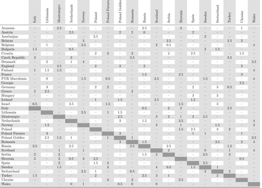
In both tournaments the number of competing teams is 𝑛 = 38 playing on 𝑡 = 4 tables during 𝑐= 9 rounds. Results are known for about the quarter of possible pairs, 9×19 = 171 from 𝑛(𝑛−1)/2 = 703.
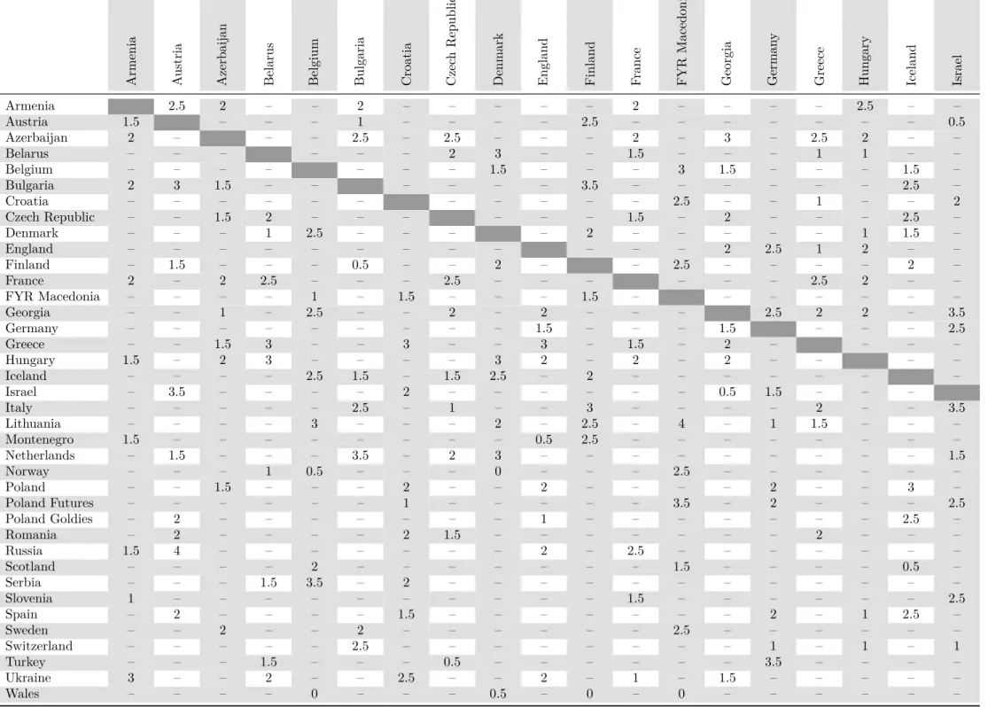
Number of board points achieved by the team in the corresponding row against the team in the corresponding column are presented in Tables A.1 (2011) and A.2 (2013) in the Appendix. At least 2.5 board points means a win, 2 means a draw, while at most 1.5 means a loss. Unplayed matches are indicated by –.
The first element of the official lexicographical order was the number of match points in both cases but tie-breaking rules were different. They certainly should be used since in 9 matches at most 18 match points can be achieved and the number of participants is 38. The first tie-breaking rule was number of board points in ETCC 2011 and Olympiad-Sonneborn- Berger points without lowest result (i.e. match points of each opponent, excluding the opponent who scored the lowest number of match points, multiplied by the number of game points achieved against this opponent) in ETCC 2013, therefore teams have had an incentive to achieve more points. It is especially relevant for middle teams. The pairing algorithm provides that a team scoring 9 wins will be the first, however, such a feat is almost impossible. To conclude, teams are interested in scoring more match points and board points, which count through the tie-breaking rules.2
In the 2013 competition application of the first tie-breaking rule (Olympiad-Sonneborn- Berger points) was enough, while in 2011 a second tie-breaking rule (aggregated board points of the opponents) should be used in some cases.
Tables A.3 (2011) and A.4 (2013) in the Appendix focus on match outcomes: 4 indicates a win for the team in the corresponding row, = and 7 indicate a draw and a loss, respectively. Match points aggregate them by giving 2 for wins, 1 for draws and 0 for losses. Teams are ordered according to the official ranking. Wins are usually above the diagonal and played matches tend to be placed close to the diagonal because of the concept of the pairing algorithm.
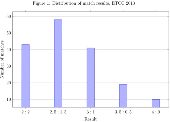
Distribution of match results for ETCC 2013 is drawn in Figure 1. Minimal victory (2.5 : 1.5) is the mode, so incorporating board points probably will not influence the
rankings much.
We have two exogenous rankings calledOfficial according to the tournament rules and Start based on ´El˝o points of players, reflecting the past performance of team members.
Further 12 rankings have been calculated from the ranking problem representation. Four results matrices have been considered: 𝑅𝑀 𝑃, 𝑅𝑀 𝐵 = 𝑅𝑃(1/4) = 3/4𝑅𝑀 𝑃 + 1/4𝑅𝐵𝑃, 𝑅𝐵𝑀 =𝑅𝑃(2/3) = 1/3𝑅𝑀 𝑃 + 2/3𝑅𝐵𝑃 and𝑅𝐵𝑃. We have chosen three methods, least squares (𝐿𝑆) and generalized row sum with 𝜀1 = 1/324 (𝐺𝑅𝑆1) and 𝜀2 = 1/6 (𝐺𝑅𝑆2).
Note that 𝜀1 is smaller and 𝜀2 is larger than the reasonable upper bound of 1/36 when 𝑚 = 1 and𝑛 = 38.
Existence of a unique least squares solution requires connectedness of the comparison multigraph (Proposition 2), which is provided after the third round. Rankings in the first two rounds are highly unreliable, therefore they were eliminated. From the third round all methods give one, thus we have 7×13 + 1 = 92 rankings as Start remains unchanged.
Notation 2. The 14 final rankings are denoted by Start, Official;𝐺𝑅𝑆1(𝑅𝑀 𝑃),𝐺𝑅𝑆1(𝑅𝑀 𝐵), 𝐺𝑅𝑆1(𝑅𝐵𝑀), 𝐺𝑅𝑆1(𝑅𝐵𝑃); 𝐺𝑅𝑆2(𝑅𝑀 𝑃), 𝐺𝑅𝑆2(𝑅𝑀 𝐵), 𝐺𝑅𝑆2(𝑅𝐵𝑀), 𝐺𝑅𝑆2(𝑅𝐵𝑃); and
2 Sometimes leading teams can secure a prize by a draw in the final round or certain teams may lose their spirit to compete. These issues emerge in all sports, note that soccer teams in national competitions have usually weak incentives to win by a lot of goals.
Figure 1: Distribution of match results, ETCC 2013
2 : 2 2,5 : 1,5 3 : 1 3,5 : 0,5 4 : 0
10 20 30 40 50 60
Result
Numberofmatches
𝐿𝑆(𝑅𝑀 𝑃), 𝐿𝑆(𝑅𝑀 𝐵),𝐿𝑆(𝑅𝐵𝑀),𝐿𝑆(𝑅𝐵𝑃). In the figures they are abbreviated by Start, Off; G1, G2, G3, G4; S1, S2, S3, S4; and L1, L2, L3, L4, respectively.
Start and Official rankings are strict, that is, they do not allow for ties by definition.
It can be checked that the other rankings also give a linear order of teams in all cases.
Rankings by different methods are displayed in Tables A.5 (2011) and A.6 (2013) in the Appendix.
4.2 Visualisation of the rankings
For the comparison of final rankings their distances have been calculated. We have chosen the well-known Kemeny distance (Kemeny, 1959) and its weighted version proposed by Can (2014). Both distances are defined on the domain of strict rankings, i.e. ties are not allowed. Our rankings satisfy this condition. Kemeny distance was characterized by Kemeny and Snell (1962), however, Can and Storcken (2013) achieved the same result without one condition. Can and Storcken (2013) also provides an extensive overview about the origin of this measure. It is the number of pair of alternatives ranked oppositely in the two rankings examined. For instance, Kemeny distance of 𝑎 ≻𝑏 ≻𝑐 and 𝑏 ≻𝑎 ≻𝑐 is 1, because they only disagree on how to order 𝑎 and𝑏. Similarly, Kemeny distance of 𝑎≻𝑏 ≻𝑐and 𝑎 ≻𝑐≻𝑏 is 1 since the disagreement on how to order 𝑏 and 𝑐.
Thus the dissimilarity between the former two and between the latter two seems to be identical according to the Kemeny distance. However, in our chess example a disagreement at the top of the rankings may be more significant than a disagreement at the bottom of them: the audience is interested in the first three, five or ten places but people are not bothered much whether a team is the 31th or 34th. For this purpose, Can (2014) proposes some functions on strict rankings in the spirit of Kemeny metric, which are
respectful to the number of swaps but allow for variation in the treatment of different pairs of disagreements.
It has some price since the calculation will depend on the order of swaps between the two rankings. Can (2012, Theorem 1) shows that only the path-minimizing function satisfies the triangular inequality condition for all possible weight vectors. Finding the path-minimizing metric is not trivial, it is equivalent to solving a short-path problem. A way out is that if weights are monotonically decreasing (increasing) from the upper parts of a ranking to the lower parts, then the Lehmer function (the inverse Lehmer function) is equivalent to the path-minimizing metric (Can, 2014, Corollaries 1 and 2).
These results have inspired us to choose a monotonically decreasing weight vector meaning that swaps in the first places are more important than changes at the bottom of the rankings. Our weight vector is given by 𝜔𝑖 = 1/𝑖for all 𝑖= 1,2, . . . , 𝑛−1. Then the distance between 𝑎 ≻𝑏 ≻ 𝑐 and 𝑏 ≻ 𝑎 ≻𝑐 is 1 (a swap at the first position), while the distance between 𝑎 ≻𝑏 ≻ 𝑐 and 𝑎 ≻𝑐 ≻𝑏 is 1/2 (a swap at the second position). The measure reaches its maximum of𝑛−1 if and only if the two rankings are entirely opposite.
We do not know about any other application of Can (2014)’s novel method.
Distances of rankings of ETCC 2011 competition is presented in Table A.7 in the Appendix. All Kemeny distances are significantly smaller than its maximum of𝑛(𝑛−1)/2 = 703 for entirely opposite rankings. Largest values usually occur in comparison with Start since it is not influenced by the results. However, rankings based on match points and board points are also relatively far from each other. Official coincides with 𝐺𝑅𝑆1(𝑅𝑀 𝐵).
Weighted distances are presented in Table A.7.b. Its maximum is 𝑛−1 = 37. Ratio of Kemeny and weighted distances are between 8.73 and 17.44 for ETCC 2011, and between 5.81 and 18.73 for ETCC 2013. In the second case accounting for swaps’ positions has a larger effect but the discrepancy of the two distances remains smaller than expected. It implies that variations are more or less equally distributed along the rankings.
It is worth to note here that 𝐺𝑅𝑆1(𝑅𝑀 𝑃) means a kind of tie-breaking rule for match points both in ETCC 2011 and ETCC 2013. If 𝜀 = 0 then generalized row sum gives the ranking of match points, while a small 𝜀 ranks tied teams by the strength of their opponents. Official method also aims to eliminate ties, it uses a different approach though.
Table A.7 gives some information, however, it does not much simplify the comparison of the rankings. We want to achieve this by a graphical representation. The pairwise distances of 14 rankings can be plotted in a 13-dimensional space without loss of information but it still seems to be unmanageable. Therefore, similarly to Csat´o (2013), multidimensional scaling (Kruskal and Wish, 1978) have been applied. It is a statistical method in information visualization for exploring similarities or dissimilarities in data: a textbook application of MDS is to draw cities on a map from the matrix consisting of their air distances.
Kemeny and weighted distances mean a ratio scale due to the existence of a natural minimum and maximum. Then discrepancies of the reduced dimensional map are linear functions of the original distances. Both Stress and RSQ tests for validity strengthen that two dimensions are sufficient to plot the 14 rankings, but one is too restrictive. The method gives a map where only the position of objects count, more similar rankings are closer to each other. Only the distances of points representing the rankings yield information, we do not know what is the meaning of the axes.3
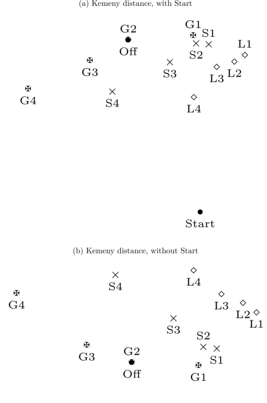
Figure 2 shows MDS maps for the 2011 tournament. Figure 2.a supports the view that Start is far away from all other rankings, thus it is omitted from further analysis (which improves the mapping, too).
3 Note the change of direction of the vertical axis on Figures 2 and 3.
Figure 2: MDS maps of the European Team Chess Championship 2011 rankings
Official ranking (Off) is the same as one from generalized row sum (G2), their distances are zero. There is a minimal difference between the coordinates of corresponding points, probably due to computational errors.
(a) Kemeny distance, with Start
∙ Start
∙ Off
@ G1
× S1
L1 ◇
@ G2
×
S2 ◇ L2
@ G3
×
S3 ◇
L3
@
G4 ×
S4 ◇
L4
(b) Kemeny distance, without Start
∙
Off @
G1
× S1
◇ L1
@
G2 S2 ×
◇ L2
@ G3
× S3
◇ L3
@ G4
× S4
◇ L4
There is not much difference between the four charts (ETCC 2011 vs. 2013, Kemeny vs. weighted distances) as Figure 3 is similar to Figure 2.b. MDS maps of ETCC 2013 an Kemeny distances have more favorable validity measures than MDS maps of ETCC 2011 and weighted distances. They suggest the following:
1. Start significantly differs from the other rankings since it does not depend on the
Figure 3: MDS maps of the European Team Chess Championship 2013 rankings (a) Kemeny distance, without Start
∙
Off @ G1
× S1
◇ L1
@ G2
S2 ×
L2 ◇
@ G3
× S3
◇
@ L3 G4
× S4
◇ L4
(b) Weighted distance, without Start
∙ Off @
G1
× S1
◇ L1
@ G2
S2 ×
L2 ◇
@ G3
S3 ×
◇
@ L3 G4
× S4
◇ L4
results of the tournament;
2. Generalized row sum rankings (with low𝜆) are more similar to the official one than least squares;
3. The order of results matrices by variance is𝑅𝑀 𝑃 < 𝑅𝑀 𝐵 < 𝑅𝐵𝑀 < 𝑅𝐵𝑃, a greater role of match points stabilize the rankings;
4. The order of scoring procedures by variance is 𝐿𝑆 < 𝐺𝑅𝑆2 < 𝐺𝑅𝑆1, a greater role of opponents stabilize the rankings.
5. Choice of tie-breaking rule for match points has a surprisingly large effect, especially in the case of ETCC 2011 as rankings Off and G1 are relatively far from each other.
On the basis of these observations, we propose to use least squares with a generalized results matrix favoring match points (a low 𝜆, for example, 1/4 as in 𝑅𝑀 𝐵) for ranking in Swiss-system chess team tournaments as it gives incentives for teams to score more board points but still prefers match points against them.
4.3 Analysis of a ranking
Another approach to compare the rankings is offered by the decomposition of the least squares rating (Csat´o, 2014a). The ranking problem is balanced, the comparison multigraph is regular. Therefore it gives a ranking according to mp(the official ranking without the application of tie-breaking rules) in the zeroth step (q(0)) as Proposition 3 states. After that, it reflects the strength of neighbors, neighbors of neighbors and so on by accounting for their average match points since d𝐼 − 𝐿 = 𝑀. Ranking according to q(𝑅𝑀 𝑃) is obtained after the seventh (from q(7)(𝑅𝑀 𝑃)) and after the twelfth step (from q(12)(𝑅𝑀 𝑃)) for ETCC 2011 and ETCC 2013, respectively.
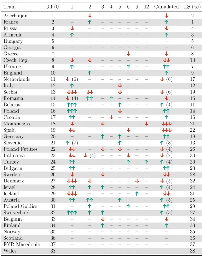
Table 1 shows the changes of teams’ positions in each step of the iterative decomposition of the ranking 𝐿𝑆(𝑅𝑀 𝑃) for ETCC 2013. In the second column ties are broken according to the official rules, so it coincides with the official ranking. In subsequent steps there are no ties. Position improvements and declines are indicated by the Ô and Ô
arrows, respectively. Lack of change is indicated by –.
Correction according to neighbors’ strength results in seven positions improvement for Slovenia together with a four positions decline for Romania and six for Netherlands. Hence Slovenia overtakes Netherlands despite it has a two match points disadvantage. Official tie-breaking rule 𝑇 𝐵4 (number of board points of the opponents) shows a similar direction of adjustment. Subsequent steps of the iteration usually lead to a similar sign of change in positions, however, in a more moderated extent. A notable exception is Romania, which regains some positions due to indirect opponents. Monotonicity of absolute adjustments are violated only by Lithuania.
There are two changes among the top six teams. After 𝑘 = 2 France becomes the winner of the tournament instead of Azerbaijan. It can be debated since the latter team has no loss, however, the schedule of France was more difficult. The swap of Russia and Armenia may be explained by the advance on an outer circle of the former team. Note the lack of match between Azerbaijan and Russia (Table A.4).
The last change is a swap of Turkey and Montenegro in the twelfth step of the iteration.
As it was mentioned, least squares method is not only a tie-breaking rule for match points (contrary to generalized row sum with 𝜀= 1/324), it makes possible that a team overtakes
another one despite its disadvantage of two match points.
Imperfection of the official ranking is highlighted by ETCC 2011, for which Table A.8 in the Appendix contains the positional changes according to the iterative decomposition of 𝐿𝑆(𝑅𝑀 𝑃). Here France scored three wins and three draws in the first six rounds but it has been defeated in the last three matches. It is an extreme example of advance on an inner circle, France has had a more challenging schedule compared to teams with the same number of match points. It is reflected in the significant adjustment by the least squares method. On the other side, Serbia loses nine, and Georgia loses 14 positions. They had luck with the opponents, for example, Georgia had not played against a better team according to the official ranking. We think it is a surprising fact for a team at the 13th place. You can also see that both Serbia and Georgia significantly benefits from decreasing 𝜀 or increasing the role of board points.
The strange phenomenon is also remarked by a Hungarian commentator who speaks about ’the curse of the Swiss system’.4 However, we think it is not necessarily the mistake of Swiss system rather a failure of the official ranking, which can be improved significantly
4 See at http://sakkblog.postr.hu/sokan-palyaznak-dobogos-helyezesre-izgalmas-utolso- fordulo-dont.
Table 1: Positional changes in decomposition of the ranking 𝐿𝑆(𝑅𝑀 𝑃), ETCC 2013
Team Off (0) 1 2 3 4 5 6 9 12 Cumulated LS (∞)
Azerbaijan 1 – Ô
– – – – – – Ô
2
France 2 – Ô – – – – – – Ô 1
Russia 3 Ô
– – – – – – – Ô
4
Armenia 4 Ô – – – – – – – Ô 3
Hungary 5 – – – – – – – – – 5
Georgia 6 – – – – – – – – – 6
Greece 7 – – – – – Ô
– – Ô
8
Czech Rep. 8 Ô Ô
– – – – – – Ô Ô
10
Ukraine 9 Ô – – – – Ô – – Ô Ô 7
England 10 – Ô – – – – – – Ô 9
Netherlands 11 Ô
(6) – – – – – – – Ô
(6) 17
Italy 12 Ô – – – Ô
– – – – 12
Serbia 13 Ô Ô Ô Ô Ô
– – Ô
– – – Ô
(6) 19
Romania 14 Ô
(4) Ô Ô – Ô – – – – Ô
15
Belarus 15 Ô Ô Ô – – – Ô – – – Ô (4) 11
Poland 16 Ô Ô Ô – – – Ô
– – – Ô Ô 14
Croatia 17 Ô Ô – – Ô
– – – – Ô 16
Montenegro 18 Ô
– Ô
– – – – Ô Ô Ô Ô
21
Spain 19 Ô Ô
– – – – Ô
– – Ô Ô Ô
22
Germany 20 – – Ô – Ô – – – Ô Ô 18
Slovenia 21 Ô (7) – – – Ô – – – Ô (8) 13
Poland Futures 22 Ô Ô
– Ô
– Ô
– – – Ô
(4) 26
Lithuania 23 Ô Ô Ô
(4) – – – Ô
– – Ô
(7) 30
Turkey 24 Ô Ô – – – – Ô – Ô Ô (4) 20
Bulgaria 25 Ô Ô – – – – – – – Ô Ô 23
Sweden 26 Ô
– Ô
– – – – – Ô Ô
28
Denmark 27 Ô Ô Ô Ô
– – – – Ô
– Ô
(5) 32
Israel 28 Ô Ô Ô Ô – – – – – Ô (4) 24
Iceland 29 Ô Ô Ô
– – – – – Ô – Ô Ô
31
Austria 30 Ô Ô Ô Ô – – Ô – – – Ô (5) 25
Poland Goldies 31 – Ô – – – Ô – – Ô Ô 29
Switzerland 32 Ô Ô Ô Ô Ô – – – – – Ô (5) 27
Belgium 33 – – Ô
– – – – – Ô
34
Finland 34 – – Ô – – – – – Ô 33
Norway 35 – – – – – – – – – 35
Scotland 36 – – – – – – – – – 36
FYR Macedonia 37 – – – – – – – – – 37
Wales 38 – – – – – – – – – 38
by accounting for the strength of opponents.
4.4 Assessment of the rankings
For evaluating the 14 rankings, three approaches have been applied:
∙ Predictive performance: ability to forecast the outcomes of future matches;
∙ Retrodictive performance: ability to match the results of contests already played;
∙ Robustness between subsequent rounds.
The first two are the proposals of Pasteur (2010) for the classification of mathematical ranking models. The third seems to be important because of (at least) two causes. First, both the participants and the audience feel strange if the positions of teams are not stable, they are largely determined by a certain match result. Naturally, extreme stability is not favorable, too, but it is usually not a problem in a Swiss system tournament. The second argument for robustness is that the number of rounds is often determined arbitrarily, for instance, it was 13 in the 2006 and 11 in the 2013 chess olympiads with 148 and 146 teams, respectively.
The first two have been measured by the number of match and board points scored by an underdog against a better team. It does not take into account the difference of positions, only its sign. Some results are presented in the Appendix. They are qualitatively equivalent, the methods applied behave similarly in all cases.
Figure A.1 shows the number of match and board points scored by a weaker opponent in later rounds according to the appropriate ranking after each round. It can be calculated from the third round when the least squares ranking is unique. Start has the most favorable forecasting performance, especially in the first rounds, match outcomes are determined by teams’ ability rather than by their results in the competition. As Figure A.2 reveals, there is no difference among the methods in forecasting power if only the next round is scrutinized, too.
Forecasting can be regarded as out-of-sample fit. Another approach is how a ranking describes the results of matches already played, that is, in-sample fit. Figure A.3 shows the number of match and board points in earlier rounds scored by a weaker opponent according to the appropriate ranking after each round. It is calculated from the third round, however, it has a meaning after the last round when forecasting power is not defined. Least squares method has the best retrodictive performance but it remains dubious whether it is statistically significant. Generalized row sum is placed between the least squares and official rankings. Choice of the results matrix and the tournament does not influence these findings.
Stability has been defined as the distance of rankings in subsequent rounds. It has no meaning for Start but can be calculated for all other rankings from the third round.
Figure 4 illustrates the robustness of some rankings in ETCC 2011. Volatility is not monotonically decreasing, however, a stable decline is observed as the actual round gives relatively fewer and fewer information. Ranking 𝐿𝑆(𝑅𝑀 𝑃) is the most robust according to both definitions of the distance, which is followed by 𝐺𝑅𝑆2(𝑅𝑀 𝑃), then 𝐺𝑅𝑆1(𝑅𝑀 𝑃) and Official. Therefore rankings become less volatile by taking into account the performance of opponents. Difference of absolute values is more significant in the case of weighted distance, the least squares method is more robust in the first, critical places. The order 𝐿𝑆 < 𝐺𝑅𝑆2 < 𝐺𝑅𝑆1 is valid for other result matrices 𝑅𝑀 𝐵, 𝑅𝐵𝑀 and 𝑅𝐵𝑃, however, 𝐺𝑅𝑆1 is sometimes worse than the official ranking.
Results for ETCC 2013 are presented on Figure A.4 in the Appendix. Now the conclusions are more uncertain but least squares is the most stable with the exception of first rounds. To summarize, application of the least squares method is recommended if the organizers want to mitigate the effects of the (predetermined) number of rounds on the ranking.
Figure 4: Stability between rounds, ETCC 2011 (a) Kemeny distance, results matrix 𝑅𝑀 𝑃
3−4 4−5 5−6 6−7 7−8 8−9
10 20 30 40 50 60 70 80 90 100
Off
G1 S1
L1
Off G1 S1 L1
(b) Weighted distance, results matrix𝑅𝑀 𝑃
3−4 4−5 5−6 6−7 7−8 8−9
1 2 3 4 5 6 7 8 9
Off
G1 S1
L1
Off G1 S1 L1
5 Discussion
The paper has given an axiomatic analysis of ranking in Swiss system chess team tour- naments. We have applied the paired-comparison based ranking methodology in order to build an appropriate model for these competitions, which reveals the failure of official lexicographical rankings. The framework is flexible with respect to the role of the oppo- nents (parameter 𝜀) and the influence of match and board points (choice of the results matrix). The main theoretical advantages of the methods proposed are that they are close to the concept of official rankings (in fact they coincide in the case of round-robin tournaments), can be calculated iteratively or by solving a system of linear equations and have a clear interpretation on the comparison multigraph. They also do not call for arbitrary tie-breaking rules.
It is tested on the results of the 2011 and 2013 European Team Chess Championship open tournaments. Our observations support the use of least squares method. However, it is an opportunity to take into account the number of board points scored by a generalized results matrix favoring match points (small 𝜆 close to zero). The findings suggest that official lexicographical orders have significant disadvantages, and recursive methods similar to generalized row sum and least squares are worth to consider for ranking purposes. Brozos- V´azquez et al. (2010) recommend them as tie-breaking rules in Swiss system tournaments, achievable by the choice of a small 𝜀. Brozos-V´azquez et al. (2010) summarizes their favorable properties as using all available information of the tournament to break the ties and that it is difficult players remain tied after their application.
We have presented that the idea of recursive methods can be extended and they can serve not only as a tie-breaking rule but as a unique ranking procedure. In this case the ranking will be less dependent on the designation of table or board points for the benchmark (actually, middle paths can be chosen), and will be more robust with respect to new results, increasing the reliability of the final ranking. These advantages over lexicographical methods are far less significant if generalized row sum is only used for tie-breaking with a small 𝜀.
Brozos-V´azquez et al. (2010) list three main disadvantages of recursive tie-breaking methods:
∙ Lot of people criticizes the fact that a computer is needed in order to calculate the tie-break in the tournament.
∙ In the same lines, it is also criticized that it will be difficult for the players to verify (and understand) the tie-breaks at the end of the tournament.
∙ Up to 4 or 5 rounds might be needed for the methods to be convergent. Hence, intermediate standings prior to that round cannot incorporate the tie-break.
According to our view, the third point does not mean such a serious problem since rankings in the first rounds are obviously not reliable and other tie-breaking rules may be applied, e.g. ´El˝o points. In the tournaments examined, connectedness of the comparison multigraph is provided after the third round. We have also seen that the rankings after one or two iteration steps are not very far from the final ranking and they can be calculated by hand. Naturally, the least squares method is a bit more complicated than usual tie-breaking rules but its graph interpretation (Csat´o, 2014a) and its core concept close to Buchholz helps in the understanding. Anyway, there usually exists a trade-off between simplicity and other favorable properties (like sample fit, robustness), and we think it is worth to
use more developed methods in the case of Swiss system tournaments in order to avoid anomalies of the ranking.5
There are some plausible area of further research. In the analysis we have neglected some complications observed in practice like matches played with black or white (an unavoidable issue in individual tournaments) or different number of matches due to byes or unplayed games. The choice of parameter 𝜀 also requires further investigation. Our findings can be strengthened or falsified by the examination of other competitions and some simulations of Swiss system tournaments.
Finally we mention two possible use of the proposed ranking method. First, it can be incorporated into the pairing algorithm, which may lead to more balanced schedules.
Second, extensive analysis of the stability of a ranking between subsequent rounds may contribute to the choice of the number of rounds: it can be made endogenous as a function of the number of participants and other restrictions.
Acknowledgements
The research was supported by OTKA grant K 111797.
This research was supported by the European Union and the State of Hungary, co-financed by the European Social Fund in the framework of T ´AMOP 4.2.4. A/1-11-1-2012-0001
’National Excellence Program’.
References
S. Boz´oki, J. F¨ul¨op, and L. R´onyai. On optimal completion of incomplete pairwise comparison matrices. Mathematical and Computer Modelling, 52(1-2):318–333, 2010.
S. Boz´oki, L. Csat´o, L. R´onyai, and J. Tapolcai. Robust peer review decision process.
Manuscript, 2014.
M. Brozos-V´azquez, M. A. Campo-Cabana, J. C. D´ıaz-Ramos, and J. Gonz´alez-D´ıaz.
Recursive tie-breaks for chess tournaments. 2010. URL http://eio.usc.es/pub/
julio/Desempate/Performance_Recursiva_en.htm.
B. Can. Weighted distances between preferences. Technical Report RM/12/056, Maas- tricht University School of Business and Economics, Graduate School of Business and Economics, 2012.
B. Can. Weighted distances between preferences. Journal of Mathematical Economics, 51:
109–115, 2014.
B. Can and T. Storcken. A re-characterization of the Kemeny distance. Technical Report RM/13/009, Maastricht University School of Business and Economics, Graduate School of Business and Economics, 2013.
P. Chebotarev. An extension of the method of string sums for incomplete pairwise comparisons (in Russian). Avtomatika i Telemekhanika, 50(8):125–137, 1989.
5 An excellent example is Georgia’s 13th place in ETCC 2011 such that it have not played any teams better according to the official ranking.
P. Chebotarev. Aggregation of preferences by the generalized row sum method. Mathe- matical Social Sciences, 27(3):293–320, 1994.
P. Chebotarev and E. Shamis. Characterizations of scoring methods for preference aggregation. Annals of Operations Research, 80:299–332, 1998.
P. Chebotarev and E. Shamis. Preference fusion when the number of alternatives exceeds two: indirect scoring procedures. Journal of the Franklin Institute, 336(2):205–226, 1999.
L. Csat´o. A pairwise comparison approach to ranking in chess team championships. In P. F¨ul¨op, editor,Tavaszi Sz´el 2012 Konferenciak¨otet, pages 514–519. Doktoranduszok Orsz´agos Sz¨ovets´ege, Budapest, 2012.
L. Csat´o. Ranking by pairwise comparisons for Swiss-system tournaments. Central European Journal of Operations Research, 21(4):783–803, 2013.
L. Csat´o. A graph interpretation of the least squares ranking method. Social Choice and Welfare, 2014a. URL http://link.springer.com/article/10.1007%2Fs00355-014-
0820-0. Forthcoming.
L. Csat´o. Additive and multiplicative properties of scoring methods for preference aggre- gation. Corvinus Economics Working Papers 3/2014, Corvinus University of Budapest, Budapest, 2014b.
H. A. David. Ranking from unbalanced paired-comparison data.Biometrika, 74(2):432–436, 1987.
ECU. Tournament Rules, 2012. URL http://europechess.net/index.php?option=
com_content&view=article&id=9&Itemid=15. European Chess Union.
ECU. European Team Chess Championship 2013. Tournament Rules, 2013. URL http://etcc2013.com/wp-content/uploads/2013/06/ETCC-2013-tournament- rules-June-06-2013.pdf. European Chess Union.
FIDE. Handbook, 2014. URLhttp://www.fide.com/fide/handbook.html. F´ed´eration Internationale des ´Echecs (World Chess Federation).
J. Gonz´alez-D´ıaz, R. Hendrickx, and E. Lohmann. Paired comparisons analysis: an axiomatic approach to ranking methods. Social Choice and Welfare, 42(1):139–169, 2014.
V. M. Jeremic and Z. Radojicic. A new approach in the evaluation of team chess championships rankings. Journal of Quantitative Analysis in Sports, 6(3):Article 7, 2010.
X. Jiang, L.-H. Lim, Y. Yao, and Y. Ye. Statistical ranking and combinatorial Hodge theory. Mathematical Programming, 127(1):203–244, 2011.
H. F. Kaiser and R. C. Serlin. Contributions to the method of paired comparisons. Applied Psychological Measurement, 2(3):423–432, 1978.
J. G. Kemeny. Mathematics without numbers. Daedalus, 88(4):577–591, 1959.
J. G. Kemeny and L. J. Snell. Preference ranking: an axiomatic approach. InMathematical models in the social sciences, pages 9–23. Ginn, New York, 1962.
J. B. Kruskal and M. Wish. Multidimensional scaling. Sage Publications, Beverly Hills and London, 1978.
E. Kujansuu, T. Lindberg, and E. M¨akinen. The stable roommates problem and chess tournament pairings. Divulgaciones Matem´aticas, 7(1):19–28, 1999.
E. Landau. Zur relativen Wertbemessung der Turnierresultate. Deutsches Wochenschach, 11:366–369, 1895.
E. Landau. ¨Uber Preisverteilung bei Spielturnieren. Zeitschrift f¨ur Mathematik und Physik, 63:192–202, 1914.
P. S. H. Leeflang and B. M. S. van Praag. A procedure to estimate relative powers in binary contacts and an application to Dutch Football League results. Statistica Neerlandica, 25(1):63–84, 1971.
Snj´olfur ´Olafsson. Weighted matching in chess tournaments. Journal of the Operational Research Society, 41(1):17–24, 1990.
R. D. Pasteur. When perfect isn’t good enough: Retrodictive rankings in college football.
In J. A. Gallian, editor, Mathematics & Sports, Dolciani Mathematical Expositions 43, pages 131–146. Mathematical Association of America, Washington, DC, 2010.
A. Rubinstein. Ranking the participants in a tournament. SIAM Journal on Applied Mathematics, 38(1):108–111, 1980.
E. Shamis. Graph-theoretic interpretation of the generalized row sum method. Mathemat- ical Social Sciences, 27(3):321–333, 1994.
R. T. Stefani. Improved least squares football, basketball, and soccer predictions. IEEE Transactions on Systems, Man, and Cybernetics, 10(2):116–123, 1980.
E. Zermelo. Die Berechnung der Turnier-Ergebnisse als ein Maximumproblem der Wahrscheinlichkeitsrechnung. Mathematische Zeitschrift, 29:436–460, 1929.