Solution of the Least Squares Method problem of pairwise comparison matrices
Sándor Bozóki 1 Abstract
The aim of the paper is to present a new global optimization method for determining all the optima of the Least Squares Method (LSM) problem of pairwise comparison matrices. Such matrices are used, e.g., in the Analytic Hierarchy Process (AHP). Unlike some other distance minimizing methods, LSM is usually hard to solve because of the corresponding nonlinear and non-convex objective function. It is found that the optimization problem can be reduced to solve a sys- tem of polynomial equations. Homotopy method is applied which is an efficient technique for solving nonlinear systems. The paper ends by two numerical example having multiple global and local minima.
1 Introduction
In Multi-Attribute Decision Making, one of the central questions is deter- mining the weights of attributes (criteria) or the cardinal preferences of the alternatives (actions). Usually, the decision makers may be requested to tell neither the explicit weights of the criteria representing the importance, nor the cardinal preferences of the alternatives, but they can make pairwise com- parisons. Condorcet [11] and Borda [3] used pairwise comparisons in the 18th century, as well as Weber and Fechner [17] in experimental psychology in the second half of the 19th century, then Thorndike [30] and Thurstone [31] in the 1920’s.
The method of pairwise comparisons using ratio scale was developed by Thomas L. Saaty [28]. Using the Analytic Hierarchy Process (AHP), difficult decision problems can be broken into smaller parts by the hierarchi- cal criterion-tree, one level of the tree can be handled by pairwise comparison matrices.
1Laboratory of Operations Research and Decision Systems Computer and Automation Institute, Hungarian Academy of Sciences, 1518 Budapest P.O. Box 63, Hungary,E-mail:
bozoki@oplab.sztaki.hu
This research was supported in part by the Hungarian Scientific Research Fund, Grant No. OTKA K 60480.
Manuscript of / please cite as Bozóki, S. [2008]:
Solution of the Least Squares Method problem of pairwise comparison matrices, Central European Journal of Operations Research 16, pp.345-358.
DOI 10.1007/s10100-008-0063-1
http://www.springerlink.com/content/b2257h112256v32n
A pairwise comparison matrix A = [aij]i,j=1..n is defined as
A =
1 a12 a13 . . . a1n
a21 1 a23 . . . a2n
a31 a32 1 . . . a3n
... ... ... ... ...
an1 an2 an3 . . . 1
∈Rn×n+ ,
where Rn×n+ denotes the class of positive n×n matrices, and for any i, j = 1, . . . , n,
aij >0, aij = 1 aji
.
The matrix element aij expresses the relative importance or preference of i-th object compared to j-th object given by the decision maker (i, j = 1,2, . . . , n). For example, the first object isa12times more important/preferred than the second one.
An A = [aij]i,j=1..n pairwise comparison matrix is called consistent, if it satisfies the following properties for all indices i, j, k = 1, . . . , n:
aij = 1 aji
, aijajk=aik.
In practical decision problems, pairwise comparison matrices given by the decision maker are not consistent. Based on the elements of the matrix, we want to find a weight vector w = (w1, w2, . . . , wn)T ∈ Rn+ representing the priorities of the objects where Rn+ is the positive orthant. The Eigenvec- tor Method [28] and some distance minimizing methods such as the Least Squares Method [9, 24], Logarithmic Least Squares Method [14, 13, 12, 1], Weighted Least Squares Method [9, 2], Chi Squares Method [24], Logarith- mic Least Absolute Values Method [10, 23] and Singular Value Decomposi- tion [21] are some of the tools for computing the priorities of the alternatives.
After some comparative analyses [8, 29, 12, 32], one of the most compre- hensive review was done by Golany and Kress [22]. They compared some scaling methods from the first 10-15 year history of pairwise comparison ma- trices by seven criteria and concluded that every method has advantages and weaknesses, none of them is prime.
Since LSM problem was not solved fully, comparisons to other methods are restricted to a few specific examples.
The aim of the paper is to present a new global optimization method for solving the LSM problem for matrices up to the size 8×8 in order to ground for further research of comparisons to other methods and examining its real life application possibilities. It is shown that the first order neces- sary conditions of optimality can be transformed to a system of multivariate polynomials. Homotopy method is applied for finding all the solutions of the polynomial system, from which all the local and global optima of the objective function can be computed [6].
In the paper we study the Least Squares Method (LSM) which is a min- imization problem of the Frobenius norm of (A−w1
w
T),where w1T denotes the row vector (w11,w12, . . . ,w1
n).
Least Squares Method (LSM) min
n
X
i=1 n
X
j=1
aij− wi
wj
2
s.t.
n
X
i=1
wi = 1, (1)
wi >0, i= 1,2, . . . , n.
LSM is rather difficult to solve because the objective function is non- linear and usually nonconvex, moreover, no unique solution exists [24, 25]
and the solutions are not easily computable. Newton’s method of successive approximation can be applied [16], but a good initial point is required.
Sufficient conditions of convexity of theLSM objective function over the feasible set are given and branch-and-bound method is applied for the gen- eral case in [18].
The transformation of the first-order conditions of optimality into a mul- tivariate polynomial system is described in Section 2. Properties of the poly- nomial sytems from the LSM problem are characterized and three methods for finding all the positive real solutions of them are given in Section 3. Nu- merical examples of Section 4 are to illustrate the complexity of the LSM problem as the dimension number increases. It is noted in Section 5 that the methods in Section 2 and 3 may be generalized into the case of incom- plete pairwise comparison matrices. Two examples of Section 6 show that the number of solutions of the LSM problem may be equal to or even twice as many as the dimension of the matrix. The paper ends by the conclusions of Section 7.
2 The LSM problem
Let A be ann×n matrix obtained from pairwise comparisons in the form
A=
1 a12 a13 . . . a1n
1/a12 1 a23 . . . a2n
1/a13 1/a23 1 . . . a3n
... ... ... . .. ...
1/a1n 1/a2n 1/a3n . . . 1
.
The aim is to find a positive reciprocal consistent matrix X in the form
X=
1 w1/w2 w1/w3 . . . w1/wn
w2/w1 1 w2/w3 . . . w2/wn
w3/w1 w3/w2 1 . . . w3/wn
... ... ... . .. ... wn/w1 wn/w2 wn/w3 . . . 1
,
which minimizes the square of the Frobenius norm kA−Xk2F =
n
X
i=1 n
X
j=1
aij − wi
wj
2 ,
subject to
n
X
i=1
wi = 1, (2)
w1, w2, . . . , wn > 0. (3)
New variables x1, x2, . . . , xn−1 are introduces as follows:
x1 = w1
w2
, x2 = w1
w3
, . . . , xi = w1
wi+1
, . . . , xn−1 = w1
wn
. (4)
The inverse formulas are computed from equations (2) and (4):
w1 = 1
1 +
n−1
P
j=1 1 xj
, wi =
1 xi−1
1 +
n−1
P
j=1 1 xj
, i= 2,3, . . . , n. (5)
Based on formulas (4) matrix X can be written as
X=
1 x1 x2 . . . xn−1
1/x1 1 x2/x1 . . . xn−1/x1
1/x2 x1/x2 1 . . . xn−1/x2
... ... ... . .. ... 1/xn−1 x1/xn−1 x2/xn−1 . . . 1
, (6)
and the LSM optimization problem (1) is reduced to min f(x1, x2, . . . , xn−1)
s.t. x1, x2, . . . , xn−1 >0, (7) where
f(x1, x2, . . . , xn−1) =kA−X k2F =
n
X
j=2
"
(a1j −xj−1)2+ 1
a1j
− 1 xj−1
2# +
+
n−1
X
i=2 n
X
j=i+1
"
aij − xj−1
xi−1
2 +
1 aij
− xi−1
xj−1
2# .
(8)
The first summation in (7) comes from the first row and column of ma- trices A and X while the second summation corresponds to the elements of the right-down (n−1)×(n −1) submatrices. Since f is a continuously differentiable function on the feasible region, the first order necessary condi- tion of local optimality are as follows:
∂f
∂x1
= ∂f
∂x2
=· · ·= ∂f
∂xn−1
= 0. (9)
The first-order partial derivatives off are rational functions ofx1, x2, . . . , xn−1
and can be transformed into multivariate polynomials. One can check by us- ing Maple that the denominator of ∂x∂f
i has the form xi
n−1
Y
j=1
xj
2, i= 1,2, . . . , n−1, (10)
and all the nominators of ∂x∂f
i-s (i = 1,2, . . . , n−1) contain a multiplier 2.
Let P1, P2, . . . , Pn−1 be defined as follows:
Pi(x1, x2, . . . , xn−1) = 1 2xi
n−1
Y
j=1
xj 2
! ∂f
∂xi
, i= 1,2, . . . , n−1. (11)
The common zeros of polynomialsPi, (i= 1,2, . . . , n−1)are the solutions of the following system:
P1(x1, x2, . . . , xn−1) = 0;
P2(x1, x2, . . . , xn−1) = 0;
... (12)
Pn−1(x1, x2, . . . , xn−1) = 0.
Since we are interested only in positive real (x1, x2, . . . , xn−1) solutions, the systems (9) and (12) are equivalent in the sense that a positive real (n−1)-tuple(x1, x2, . . . , xn−1) is a solution of (9) if and only if it is a solu- tion of (12). This result is summarized as follows.
Proposition. All the local and global optima of the LSM problem (1) can be computed from the positive real solutions of polynomial system (12).
Example 1
Let B be a4×4 pairwise comparison matrix as follows:
B=
1 2 5 9
1/2 1 3 8
1/5 1/3 1 4 1/9 1/8 1/4 1
.
The aim is to approximate matrixBby a consistent matrixXin the form
X=
1 x1 x2 x3
1/x1 1 x2/x1 x3/x1
1/x2 x1/x2 1 x3/x2
1/x3 x1/x3 x2/x3 1
.
The reduced LSM objective function (6)-(7) is as follows:
f(x1, x2, x3) =||B−X||2F = (2−x1)2+
1
2 − 1 x1
2
+ (5−x2)2+
1
5 − 1 x2
2
+ (9−x3)2+
1
9− 1 x3
2
+
3−x2
x1
2
+
1
3 −x1
x2
2
+
8−x3
x1
2
+
1
8 −x1
x3
2
+
4− x3
x2
2
+
1
4− x2
x3
2
.
Multiplying the partial derivatives
∂f
∂x1
=−4 + 2x1+ 2
1 2− x1
1
x12 + 2
3−xx2
1
x2
x12 + 2
8−xx3
1
x3
x12 − 2
1 3 −xx1
2
x2
− 2
1 8 −xx1
3
x3
;
∂f
∂x2
=−10 + 2x2− 2
3−xx21 x1
+ 2
1 5 −x12
x22 + 2
1 3 −xx12
x1
x22 + 2
4−xx32 x3
x22 − 2
1 4 −xx23
x3
;
∂f
∂x3
=−18 + 2x3− 2
8−xx3
1
x1
− 2
4−xx3
2
x2
+ 2
1 9 −x1
3
x32 + 2
1 8 −xx1
3
x1
x32 + 2
1 4 −xx2
3
x2
x32
by x31x22x23, x21x32x23 and x21x22x33, respectively, one gets the polynomial sys- tem of three equations and three variables:
P1(x1, x2, x3) =−2x13
x22
x32
+x14
x22
x32
+1 2x1x22
x32
−x22
x32
+ 3x1x23
x32
−x24
x32
+ 8x1x2
2x3 3−x2
2x3 4−1
3x1 3x2x3
2+x1 4x3
2− 1 8x1
3x2
2x3+x1 4x2
2 = 0;
P2(x1, x2, x3) =−5x23
x12
x32
+x24
x12
x32
−3x1x23
x32
+x24
x32
+ 1 5x2x12
x32
−x12
x32
+ 1
3x13
x2x32
−x14
x32
+ 4x2x12
x33
−x12
x34
− 1 4x23
x12
x3+x24
x12
= 0 P3(x1, x2, x3) =−9x33
x12
x22
+x34
x12
x22
−8x1x22
x33
+x22
x34
−4x2x12
x33
+x12
x34
+ 1
9x3x1 2x2
2−x1 2x2
2+1 8x1
3x2
2x3−x1 4x2
2+1 4x2
3x1
2x3−x2 4x1
2= 0.
Algorithms of solving polynomial systems such as the one above, as well as a few properties regarding the degrees of the polynomials are presented in the next section.
3 Polynomial systems
A few properties of the objective functions and the polynomial systems com- puted from LSM-problem of pairwise comparison matrices are summarized in this section.
The following definitions are used. The total/minimal degree of a multi- variate polynomial can be gotten by adding the exponents of the variables in every term, and taking the maximum/minimum. For example, the poly- nomial x1x22+x41x32+x51x2 has total degree 7 and minimal degree 3.
By using the symbolic computations of Maple, one can find the properties of the polynomial systems (12) as follows:
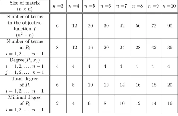
Size of matrix
(n×n) n=3 n=4 n=5 n=6 n=7 n=8 n=9 n=10 Number of terms
in the objective functionf
(n2−n)
6 12 20 30 42 56 72 90
Number of terms inPi i= 1,2, . . . , n−1
8 12 16 20 24 28 32 36
Degree(Pi, xj) i= 1,2, . . . , n−1 j= 1,2, . . . , n−1
4 4 4 4 4 4 4 4
Total degree of Pi i= 1,2, . . . , n−1
6 8 10 12 14 16 18 20
Minimal degree of Pi i= 1,2, . . . , n−1
2 4 6 8 10 12 14 16
Table 1. Properties of polynomial systems, n = 3,4, . . . ,10.
As Table 1 shows, the polynomial systems (12) have some properties of symmetry. Deg(Pi, xj)=4 for any i = 1,2, . . . , n−1, j = 1,2, . . . , n−1 indices and for any sizen. For a fixed sizen, both the total and the minimal degree of Pi and the number of terms in Pi are independent from i.
Polynomial systems are not easy to solve in general. The method based on Gröbner bases [7] in Maple (Groebner Package) works for the 3×3 ma- trices but runs out of memory as n >3. A method based on resultants was given for solving the LSM problem for 3×3 matrices [4], and another one with Robert H. Lewis [5] based on generalized resultants for 4×4 matrices.
Homotopy continuation method is a general technique for solving non- linear systems proposed by Drexler [15] Garcia, Zangwill [20]. Homotopy method is based on that if two non-linear systems have the same the number of roots, then the roots can be corresponded to each other and the path from a root to another one is a continuous trajectory or homotopy. The homotopy connects the nonlinear system to be solved with another system which is already solved. In the paper, the code written by Tien-Yien Li and Tangan Gao2 [27, 19] is used.
4 Numerical experiences
This section presents the solution of Example 1 in Section 1 followed by test results based on pairwise comparison matrices of size 3×3,4×4, . . . ,8×8.
The polynomial system derived from Example 1 in Section 2 has 212 solutions, 16 of which are real and there exist only one positive solution:
x⋆1 = 1.23095456;
x⋆2 = 3.88538906;
x⋆3 = 9.57889668.
Consequently, x⋆1, x⋆2, x⋆3 is the only stationary point of reduced LSM ob- jective function of Example 1. The Hessian matrix of f is positive definite in (x⋆1, x⋆2, x⋆3), and from formulas (5), the optimal solution of theLSM problem is
wLSM1 = 0.460;
wLSM2 = 0.374;
wLSM3 = 0.118;
wLSM4 = 0.048.
It is observed that the complexity of the LSM problem arises quickly as the dimension of the matrix increases: both the number of solutions of the polynomial systems and the CPU time grows exponentially. Table 2 presents some technical information about the solutions of polynomial systems from pairwise comparison matrices of sizes 3×3, . . . , 8×8. A processor of 1GHz with 1Gbyte memory is used3.
3The author thanks the National Information Infrastructure Development Program (NIIF) for the Supercomputer Service.
Size of matrix
(n×n) n=3 n=4 n=5 n=6 n=7 n=8
CPU time 0.05 sec 0.5 sec 20 sec 14 min 10 hours 3 days Number of
common 24 224 1640 O(104) O(105) O(106)
roots Number of
real common 4–10 8–18 16–46 32–76 64–92 128–160
roots Number of
positive real 1–7 1–11 1–31 1–15 1–28 1–21
common roots Number of
local 0–1 0–3 0–5 0–5 0–7 0–7
minima Number of
global 1–3 1–4 1–5 1–6 1–7 1–8
minima Total
number of 1–4 1–4 1–10 1–6 1–14 1–8
minima
Table 2. Solutions of polynomial systems, n= 3,4, . . . ,8.
Data in Table 2 come from the experiences with some thousands of mat- rices, some entries might be improved by analyzing more matrices and by finding specific examples.
5 LSM problem for incomplete pairwise com- parison matrices
If a decision maker hasnobjects to compare, he/she needs to fill inn(n−1)/2 elements of the upper triangular submatrix of then×npairwise comparison matrix. This number quickly increases by n, e.g., for n = 10 the decision maker is requested to make 45 comparisons.
The Least Squares approximation of a pairwise comparison matrix has the advantage that it can be used in cases of missing elements, too. If the value in the (i, j)-th position of the matrix is unknown, we simply skip the corresponding term
aij − wwi
j
2
from the objective function (1) or the term aij − xxj−1
i−1
2
in (8).
In the case of incomplete pairwise comparison matrices, theLSM problem is as follows:
min
n
X
i, j= 1 aijis known
aij − wi
wj
2
s.t.
n
X
i=1
wi = 1, (1’)
wi >0, i= 1,2, . . . , n.
Steps (4)-(8) may be applied also in the incomplete case with the mod- ification that only the pairs of indices (i, j) are considered in summation in (8) for which the values of aij are known. Based on symbolic computations of Maple, the denominator of ∂x∂f
i is x3i ·
n−1
Y
j= 1 j6=i aijis known
xj
2, i= 1,2, . . . , n−1 (9’)
and, similarly to the complete case, all the nominators of ∂x∂f
i-s (i= 1,2, . . . , n−1) contain a multiplier 2. Consequently, the modification of step (10) is as fol- lows:
Pi(x1, x2, . . . , xn−1) = 1 2
∂f
∂xi
x3i
n−1
Y
j= 1 j6=i aijis known
xj
2 (10’)
Example 2
Let us Cbe a4×4incomplete pairwise comparison matrix similar to matrix B in Example 1 but two elements and their reciprocals are omitted:
C=
1 2 9
1/2 1 3
1/3 1 4
1/9 1/4 1
.
f(x1, x2, x3) =||C−X||2F = (2−x1)2 + 1
2 − 1 x1
2
+ (9−x3)2+ 1
9 − 1 x3
2 +
3− x2
x1
2 +
1 3− x1
x2
2 +
4− x3
x2
2 +
1 4 − x2
x3
2 . Partial derivatives off can be written as
∂f
∂x1
=−4 + 2x1+ 2
1 2 −x1
1
x12 + 2
3−xx2
1
x2
x12 − 2
1 3− xx1
2
x2
;
∂f
∂x2
=− 2
3−xx21 x1
+ 2
1 3− xx12
x1
x22 + 2
4−xx32 x3
x22 − 2
1 4 −xx23
x3
;
∂f
∂x3
=−18 + 2x3− 2
4−xx32 x2
+ 2
1 9− x13
x32 + 2
1 4− xx23
x2
x32 .
After multiplication of the partial derivatives by x31x22, x21x32x23 and x22x33
respectively (note that the multipliers are different from Example 1’s), the polynomial system is
P1(x1, x2, x3) =−2x13
x22
+x14
x22
+1 2x1x22
−x22
+ 3x1x23
−x24
−1 3x13
x2+x14
; P2(x1, x2, x3) =−3x23
x1x32
+x24
x32
+1 3x2x13
x32
−x14
x32
+ 4x2x12
x33
−x12
x34
− 1 4x23
x12
x3+x24
x12
; P3(x1, x2, x3) =−9x33
x22
+x34
x22
−4x33
x2+x34
+1 9x3x22
−x22
+1 4x3x23
−x24
. The polynomial system above has 128 solutions, 8 of which are real and one of them is positive:
x⋆1 = 1.04817478;
x⋆2 = 2.53971708;
x⋆3 = 9.1562478.
Since the Hessian of f is positive definite in (x⋆1, x⋆2, x⋆3), the optimal so- lution of the LSM problem is computed from formulas (5):
wLSM1 = 0.407;
wLSM2 = 0.388;
wLSM3 = 0.160;
wLSM4 = 0.044.
The symmetrical properties regarding the number of terms and degrees of polynomial systems listed in Table 1 do not hold in the incomplete case.
However, numerical experience show that homotopy method for finding the roots of the polynomial system works as well as in the case of complete ma- trices.
What is the optimal number of pairwise comparisons if it is less than n(n −1)/2? It is an open question and the author’s opinion is that the answer should be based on both theoretical reasoning and empirical studies from real life decision problems.
6 Global and local optima
In this section, two numerical examples having multiple solutions are pre- sented. Both matrices have high inconsistency and it would be hard to find a real decision situation in which these matrices might be considered accept- able. At the same time, both have as many global optima as the dimension of the matrices, moreover, the second example has the same number of local optima, too. As it is shown, global and local optimum values may be very close to each other, which indicates the complexity of the optimization prob- lem.
Example 3
Let D be a 7×7 matrix as follows:
D=
1 8 1 1 1 1 1/8
1/8 1 8 1 1 1 1
1 1/8 1 8 1 1 1
1 1 1/8 1 8 1 1
1 1 1 1/8 1 8 1
1 1 1 1 1/8 1 8
8 1 1 1 1 1/8 1
.
There exist 7 global minimum places and the solutions have a cyclic sym- metry of the weights:
wLSM1 = (0.18757,0.08962, 0.22590, 0.07721,0.19463, 0.09299,0.13207), wLSM2 = (0.08962,0.22590, 0.07721, 0.19463,0.09299, 0.13207,0.18757), wLSM3 = (0.22590,0.07721, 0.19463, 0.09299,0.13207, 0.18757,0.08962), wLSM4 = (0.07721,0.19463, 0.09299, 0.13207,0.18757, 0.08962,0.22590), wLSM5 = (0.19463,0.09299, 0.13207, 0.18757,0.08962, 0.22590,0.07721), wLSM6 = (0.09299,0.13207, 0.18757, 0.08962,0.22590, 0.07721,0.19463), wLSM7 = (0.13207,0.18757, 0.08962, 0.22590,0.07721, 0.19463,0.09299),
f(wLSMi) = 342.721256 for i= 1,2, . . . ,7.
The existence of multiple cyclic symmetric solutions is due to the cyclic symmetry ofAand the 7 solutions result in 7 different ranks. In the next ex- ample, the number of minima is twice as many as the dimension of the matrix.
Example 4
Let E be a5×5 matrix as follows:
E=
1 6 1 1 1/6
1/6 1 6 1 1
1 1/6 1 6 1
1 1 1/6 1 6
6 1 1 1/6 1
.
There exist 5 global and 5 local minimum places and both groups of the
solutions have a cyclic symmetry:
wLSM1 = (0.28115, 0.12140,0.28693, 0.12389, 0.18663), wLSM2 = (0.12140, 0.28693,0.12389, 0.18663, 0.28115), wLSM3 = (0.28693, 0.12389,0.18663, 0.28115, 0.12140), wLSM4 = (0.12389, 0.18663,0.28115, 0.12140, 0.28693), wLSM5 = (0.18663, 0.28115,0.12140, 0.28693, 0.12389),
f(wLSMi) = 126.50024 fori= 1,2, . . . ,5,
wLSM6 = (0.10697, 0.21811,0.18711, 0.16052, 0.32730), wLSM7 = (0.21811, 0.18711,0.16052, 0.32730, 0.10697), wLSM8 = (0.18711, 0.16052,0.32730, 0.10697, 0.21811), wLSM9 = (0.16052, 0.32730,0.10697, 0.21811, 0.18711), wLSM10 = (0.32730, 0.10697,0.21811, 0.18711, 0.16052),
f(wLSMi) = 126.50148 for i= 6,7, . . . ,10.
Note that the difference between the global and the local optimum values is very small (0.00124), however, the global and the local minimum places are not close to each other at all. The 5 global and 5 local minima result in 10 different ranks. Finding the reasons of having multiple global and local optima simultaneously, may be one of the interesting questions of future re- search.
Matrices D and E have been created based on the idea of Jensen ([24], section 8. Degeneracy and Nonuniqueness of LSM Scalings) regarding3×3 pairwise comparison matrices. 3×3submatrices of pairwise comparison ma- trices of arbitrary size, which are, themselves, pairwise comparison matrices were analyzed in details by Kéri [26].
7 Conclusion
A new global optimization method for solving theLSM problem for pairwise comparison matrices is given in the paper. The LSM optimization problem is transformed to a polynomial system which can be solved by resultant method, generalized resultant method using the computer algebra system
Fermat implemented by Robert H. Lewis, or homotopy method, implemented by Tangan Gao and Tien-Yien Li. Present CPU and memory capacity allow us to solve the LSM problem up to8×8matrices. One of the advantages of LSM weighting method is that it can be used even if the pairwise comparison matrix is not completely filled in. The solution of LSM problem is not unique in general. Numerical examples show that the number of solutions of the LSM problem may be equal to or even twice as many as the dimension of the matrix.
References
[1] Barzilai, J., Cook, W.D, Golany, B. [1987]: Consistent weights for judge- ments matrices of the relative importance of alternatives, Operations Research Letters, 6, pp. 131-134.
[2] Blankmeyer, E., [1987]: Approaches to consistency adjustments,Journal of Optimization Theory and Applications, 54, pp. 479-488.
[3] Borda, J.C. de [1781]: Mémoire sur les électiones au scrutin, Histoire de l’Académie Royale des Sciences, Paris.
[4] Bozóki, S. [2003]: A method for solving LSM problems of small size in the AHP, Central European Journal of Operations Research,11, pp. 17- 33.
[5] Bozóki, S., Lewis, R. [2005]: Solving the Least Squares Method problem in the AHP for 3×3 and 4×4 matrices, Central European Journal of Operations Research, 13, pp. 255-270.
[6] Bozóki, S. [2006]: Weights from the least squares approximation of pair- wise comparison matrices (in Hungarian, Súlyok meghatározása páros összehasonlítás mátrixok legkisebb négyzetes közelítése alapján), Alkal- mazott Matematikai Lapok, 23,pp. 121-137.
[7] Buchberger, B. [1965]: On Finding a Vector Space Basis of the Residue Class Ring Modulo a Zero Dimensional Polynomial Ideal (in German), PhD Dissertation, University of Innsbruck, Department of Mathematics, Austria.
[8] Budescu, D.V., Zwick, R., Rapoport, A. [1986]: A comparison of the Eigenvector Method and the Geometric Mean procedure for ratio scal- ing, Applied Psychological Measurement, 10, pp. 69-78.
[9] Chu, A.T.W., Kalaba, R.E., Spingarn, K. [1979]: A comparison of two methods for determining the weight belonging to fuzzy sets, Journal of Optimization Theory and Applications 4, pp. 531-538.
[10] Cook, W.D., Kress, M. [1988]: Deriving weights from pairwise com- parison ratio matrices: An axiomatic approach, European Journal of Operational Research, 37, pp. 355-362.
[11] Condorcet, M. [1785]: Essai sur l’Application de l’Analyse à la Proba- bilité des Décisions Rendues á la Pluralité des Voix, Paris.
[12] Crawford, G., Williams, C. [1985]: A note on the analysis of subjective judgment matrices, Journal of Mathematical Psychology 29, pp. 387- 405.
[13] De Jong, P. [1984]: A statistical approach to Saaty’s scaling methods for priorities, Journal of Mathematical Psychology 28, pp. 467-478.
[14] DeGraan, J.G. [1980]: Extensions of the multiple criteria analysis method of T.L. Saaty (Technical Report m.f.a. 80-3) Leischendam, the Netherlands: National Institute for Water Supply. Presented at EURO IV, Cambridge, England, July 22-25.
[15] Drexler, F.J. [1978]: Eine Methode zur Berechnung sämtlicher Lösungen von Polynomgleichungssystemen, Numerische Mathematik, 29, pp. 45- 58.
[16] Farkas, A., Lancaster, P., Rózsa, P. [2003]: Consistency adjustment for pairwise comparison matrices, Numerical Linear Algebra with Applica- tions, 10, pp. 689-700.
[17] Fechner, G.T. [1860]: Elemente der Psychophysik, Breitkopf und Härtel, Leipzig.
[18] Fülöp, J. [2008]: A method for approximating pairwise comparison ma- trices by consistent matrices, Journal of Global Optimization (in print).
[19] Gao, T., Li, T.Y., Wang, X. [1999]: Finding isolated zeros of polynomial systems in Cn with stable mixed volumes, Journal of Symbolic Compu- tation, 28, pp. 187-211.
[20] Garcia, C.B., Zangwill, W.I. [1979]: Finding all solutions to polynomial systems and other systems of equations, Mathematical Programming, 16, pp. 159-176.
[21] Gass, S.I., Rapcsák, T. [2004]: Singular value decomposition in AHP, European Journal of Operational Research 154, pp. 573-584.
[22] Golany, B., Kress, M. [1993]: A multicriteria evaluation of methods for obtaining weights from ratio-scale matrices, European Journal of Operational Research, 69, pp. 210-220.
[23] Hashimoto, A. [1994]: A note on deriving weights from pairwise com- parison ratio matrices, European Journal of Operational Research, 73, pp. 144-149.
[24] Jensen, R.E. [1983]: Comparison of Eigenvector, Least squares, Chi square and Logarithmic least square meth- ods of scaling a reciprocal matrix, Working Paper 153 http://www.trinity.edu/rjensen/127wp/127wp.htm
[25] Jensen, R.E. [1984]: An Alternative Scaling Method for Priorities in Hi- erarchical Structures, Journal of Mathematical Psychology 28, pp. 317- 332.
[26] Kéri, G. [2005]: Criteria for pairwise comparison matrices (in Hungarian, Kritériumok páros összehasonlítás mátrixokra),Szigma,36, pp. 139-148.
[27] Li, T.Y. [1997]: Numerical solution of multivariate polynomial systems by homotopy continuation methods, Acta Numerica,6, pp. 399-436.
[28] Saaty, T.L. [1980]: The analytic hierarchy process, McGraw-Hill, New York.
[29] Saaty, T.L., Vargas, L.G. [1984]: Comparison of eigenvalues, logarithmic least squares and least squares methods in estimating ratios,Mathemat- ical Modeling, 5, pp. 309-324.
[30] Thorndike, E.L. [1920]: A Constant Error in Psychological Ratings, Journal of Applied Psychology, 4, pp. 25-29.
[31] Thurstone, L.L. [1927]: The Method of Paired Comparisons for Social Values, Journal of Abnormal and Social Psychology,21, pp. 384-400.
[32] Zahedi, F. [1986]: A simulation study of estimation methods in the Ana- lytic Hierarchy Process, Socio-Economic Planning Sciences,20, pp. 347- 354.