On optimal completions of incomplete pairwise comparison matrices

(1)

On optimal completions of incomplete pairwise comparison matrices

Sándor BOZÓKI^1,2 , János FÜLÖP ², Lajos RÓNYAI ³

Abstract

An important variant of a key problem for multi-attribute decision making is considered. We study the extension of the pairwise comparison matrix to the case when only partial information is avail- able: for some pairs no comparison is given. It is natural to define the inconsistency of a partially filled matrix as the inconsistency of its best, completely filled completion. We study here the uniqueness problem of the best completion for two weighting methods, the Eigen- vector Method and the Logarithmic Least Squares Method. In both settings we obtain the same simple graph theoretic characterization of the uniqueness. The optimal completion will be unique if and only if the graph associated with the partially defined matrix is connected.

Some numerical experiences are discussed at the end of the paper.

Keywords: Multiple criteria analysis, Incomplete pairwise comparison matrix, Perron eigenvalue, Convex programming

1 Introduction

Pairwise comparisons are often used in reflecting cardinal preferences, es- pecially in multi-attribute decision making, for computing the weights of criteria or evaluating the alternatives with respect to a criterion. It is assumed that decision makers do not know the weights of criteria (values of the alternatives) explicitly. However, they are able to compare any pairs of

1corresponding author

2Laboratory on Engineering and Management Intelligence, Research Group of Oper- ations Research and Decision Systems, Computer and Automation Research Institute, Hungarian Academy of Sciences; Mail: 1518 Budapest, P.O. Box 63, Hungary. Research was supported in part by OTKA grants K 60480, K 77420. E-mail: bozoki@sztaki.hu, fulop@sztaki.hu

3Informatics Laboratory, Computer and Automation Research Institute, Hungarian Academy of Sciences; and Institute of Mathematics, Budapest University of Technology and Economics. Research was supported in part by OTKA grants NK 63066, NK 72845, K77476. E-mail: ronyai@sztaki.hu

Manuscript of / please cite as

Bozóki, S., Fülöp, J., Rónyai, L. [2010]:

On optimal completions of incomplete pairwise comparison matrices, Mathematical and Computer Modelling 52, pp.318-333.

DOI 10.1016/j.mcm.2010.02.047

http://dx.doi.org/10.1016/j.mcm.2010.02.047

(2)

the criteria (alternatives). Pairwise comparison matrix [26, 27] is defined as follows. Given n objects (criteria or alternatives) to compare, the pairwise comparison matrix is A = [aij]i,j=1,...,n, where aij is the numerical answer given by the decision maker for the question ’How many times Criterion i is more important than Criterion j?’, or, analogously, ’How many times Al- ternative i is better or preferred than Alternative j with respect to a given criterion?’. A pairwise comparison matrix

A =







1 a12 a13 . . . a1n

a21 1 a23 . . . a2n

a31 a32 1 . . . a3n

... ... ... ... ...

an1 an2 an3 . . . 1







, (1)

is positive and reciprocal, i.e.,

aij > 0, aij = 1

aji

, (2)

for i, j = 1, . . . , n.

The problem is to determine the positive weight vectorw= (w1, w2, . . . , wn)^T

∈ Rⁿ+, (Rⁿ+ denotes the positive orthant of the n-dimensional Euclidean space), such that the appropriate ratios of the components of w reflect all the pairwise comparisons, given by the decision maker, as well as possible. In fact, there are several mathematical models for the objective ’as well as possible’. A comparative study of weighting methods is done by Golany and Kress [10] and a more recent one by Ishizaka and Lusti [16]. In the present paper, two well-known methods, the Eigenvector Method (EM) [26, 27] and the Logarithmic Least Squares Method (LLSM) [6, 7] are considered.

In the Eigenvector Method (EM) the approximation w^EM of w is defined by

Aw^EM =λmaxw^EM,

whereλmaxdenotes the maximal eigenvalue, also known as Perron eigenvalue, of A andw^EM denotes the the right-hand side eigenvector ofA corresponding to λmax.By Perron’s theorem,w^EM is positive and unique up to a scalar multiplication [23]. The most often used normalization is Pⁿ

i=1

w_i^EM = 1.

(3)

The Logarithmic Least Squares Method (LLSM) gives w^LLSM as the optimal solution of

min Xn

i=1

Xn

j=1

logaij −log wi

wj

2

Xn

i=1

wi = 1, (3)

wi >0, i= 1,2, . . . , n.

The optimization problem (3) is known to be solvable, and has a unique optimal solution, which can be explicitly computed by taking the geometric means of rows’ elements [7, 6].

Both the Eigenvector and Logarithmic Least Squares Methods are defined for complete pairwise comparison matrices, that is, when all then² elements of the matrix are known.

Both complete and incomplete pairwise comparisons may be modelled not only in multiplicative form (1)-(2) but also in additive way as in [8, 9, 33, 34].

Additive models of cardinal preferences are not included in the scope of this investigation. However, some of the main similarities and differences between multiplicative and additive models are indicated.

In the paper, we consider an incomplete version of the models discussed above (Section 2). We assume that our expert has given estimates aij only for a subset of the pairs (i, j). This may indeed be the case in practical situations. If the number nof objects is large, then it may be a prohibitively large task to to give as many as ⁿ₂

thoughtful estimates. Also, it may be the case that the expert agent is less certain about ranking certain pairs (i^′, j^′) than others, and is willing to give estimates only for those of the pairs, where s/he is confident enough as to the quality of the estimate.

Harker proposed a method for determining the weights from incomplete matrices, based on linear algebraic equations that could be interpreted not only in the complete case [12, 13]. Kwiesielewicz [20] considered the Logarith- mic Least Squares Method for incomplete matrices and proposed a weighting method based on the generalized pseudoinverse matrices.

A pairwise comparison matrix in (1) is calledconsistentif the transitivity aijajk = aik holds for all indices i, j, k = 1,2, . . . , n. Otherwise, the matrix

(4)

is inconsistent. However, there are different levels of inconsistency, some of which are acceptable in solving real decision problems, some are not. Mea- suring, or, at least, indexing inconsistency is still a topic of recent research [4].

Saaty [26, 27] defined the inconsistency ratio asCR = ^λmax

−n n−1

RIn ,whereλmax

is the Perron eigenvalue of the complete pairwise comparison matrix given by the decision maker, and RIn is defined as ^λ^max_n−1⁻ⁿ, where λmax is an average value of the Perron eigenvalues of randomly generatedn×npairwise comparison matrices. It is well known that λmax ≥n and equals to n if and only if the matrix is consistent, i.e., the transitivity property holds. It follows from the definition thatCR is a positive linear transformation ofλmax.According to Saaty, larger value of CR indicates higher level of inconsistency and the 10%-rule(CR≤0.10)separates acceptable matrices from unacceptable ones.

Based on the idea above, Shiraishi, Obata and Daigo [28, 29] considered the eigenvalue optimization problems as follows. In case of one missing element, denoted by x, the λmax(A(x))to be minimized:

minx>0 λmax(A(x)).

In case of more than one missing elements, arranged in vector x, the aim is to solve

minx>0 λmax(A(x)). (4) For a given incomplete matrixA, the notationsλmax(A(x))and λmax(x) are both used with the same meaning.

Pairwise comparisons may be represented not only by numbers arranged in a matrix but also by directed and undirected graphs with weighted edges [17]. A natural correspondence is presented between pairwise comparison matrices and edge weighted graphs.

A generalization of the Eigenvector Method for the incomplete case is introduced in Section 3. A basic concept of EM is that λmax is strongly related to the level of inconsistency: larger λ_max value indicates that the pairwise comparison matrix is more inconsistent. Based on this idea, the aim is to minimize the maximal eigenvalue among the complete positive reciprocal matrices extending the partial matrix specified by the agent. Here the minimum is taken over all possible positive reciprocal completions of the partial matrix. Based on Kingman’s theorem [18], Aupetit and Gen- est pointed out that when all entries of A are held constant except aij and

(5)

aji = _a¹

ij for fixedi6=j, thenλmax(A)is a logconvex (hence convex) function of logaij. We show that this result can be easily extended to the case when several entries of A are considered simultaneously as variables. This makes it possible to reformulate the maximal eigenvalue minimization problem (4) as an unconstrained convex minimization problem.

The question of uniqueness of the optimal solution occurs naturally. The first main result of the paper is solving the eigenvector optimization problem (4) and giving necessary and sufficient conditions for the uniqueness.

In Section 4, a distance minimizing method, the Logarithmic Least Squares Method (LLSM) is considered. The extension of (3) to the incomplete case appears to be straightforward. In calculating the optimal vector w we consider in the objective function the terms

logaij −log_w^wⁱ

j

2

only for those pairs (i, j) for which there exists an estimate aij.

The second main result of the paper is solving and discussing the incom- pleteLLSM problem. Analogously toEM, the same necessary and sufficient condition for the existence and uniqueness of the optimal solution is provided.

In both settings the connectedness of the associated graph characterizes the unique solvability of the problem.

Connectedness is a natural and elementary necessary condition but sufficiency is not trivial. Harker’s approximation of a missing comparison between items i and j is based on the product of known matrix elements which con- nect itoj [13]. This idea is also applied in our proof of Theorem 2. Fedrizzi and Giove apply connected subgraphs for indicating the dependence or inde- pendence of missing variables [9](Section 3., pp. 308-309). However, in the paper, the connectedness of known elements is analyzed.

The third main result of the paper is a new algorithm proposed in Section 5, based on the results of Section 3 for finding the best completion according to the EM model (i.e., with minimal λmax) of an incomplete pairwise comparison matrix. The well-known method of cyclic coordinates [3] is used.

In Section 6, numerical examples are presented for both incompleteEM and LLSM models. It is also shown that van Uden’s rule ([31],[21]) provides a very good approximation for the missing elements and may be used as a starting point for the optimization algorithm of Section 5.

All the results of the paper hold for arbitrary ratio scales including but not restricted to {1/9, . . . ,1/2,1,2, . . . ,9}proposed by Saaty [26, 27].

The conclusions of Section 7 ponder the questions of applicability from decision theoretical points of view.

(6)

2 Incomplete pairwise comparison matrices and graph representation

2.1 Incomplete pairwise comparison matrices

Let us assume that our pairwise comparison matrices are not completely given. It may happen that one or more elements are not given by the decision maker for various reasons. As we have pointed out in the Introduction, there may be several realistic reasons for this to happen.

Incomplete pairwise comparison matrices were defined by Harker [12, 13]

and investigated in [5, 20, 21, 28, 28, 30, 31]. Additive models are analyzed in [8, 9, 33, 34]. The reference list of Fedrizzi and Giove [9] is offered for more models, both multiplicative and additive.

Incomplete pairwise comparison matrix is very similar to the form (1) but one or more elements, denoted here by ∗, are not given:

A=







1 a12 ∗ . . . a1n

1/a12 1 a23 . . . ∗

∗ 1/a23 1 . . . a3n

... ... ... ... ...

1/a1n ∗ 1/a3n . . . 1







. (5)

Most of the linear algebraic concepts, tools and formulas are defined for complete matrices rather than for incomplete ones. We introduce variables x₁, x₂, . . . , xd ∈R+ for the missing elements in the upper triangular part of A.Their reciprocals, 1/x1,1/x2, . . . ,1/xd are written in the lower triangular part ofA as in (6). The total number of missing elements in matrixAis2d.

Let

A(x) =A(x1, x2, . . . , xd) =







1 a12 x1 . . . a1n

1/a12 1 a23 . . . xd

1/x₁ 1/a₂₃ 1 . . . a_3n ... ... ... ... ...

1/a1n 1/xd 1/a3n . . . 1







, (6)

where x = (x1, x2, . . . , xd)^T ∈ R^d+. The form (6) is also called incomplete pairwise comparison matrix. However, it will be useful to consider them as a class of (complete) pairwise comparison matrices as realizations of A, generated by all the values of x∈R^d+.Our notation involving variables cor- responds to the view that an incomplete pairwise comparison matrix A is actually the collection of all fully specified comparison matrices which are

(7)

identical to A at the previously specified entries.

From decision theoretical and practical points of view, the really important and exciting questions are: how to estimate weights and the level of inconsistency based on the known elements rather than somehow obtain possible, assumed, computed or generated values of the missing entries. Nev- ertheless, in many cases, ’optimal’ values of x resulted in by an algorithm may be informative as well.

2.2 Graph representation

Assume that the decision maker is asked to compare the relative importance of n criteria and s/he is filling in the pairwise comparison matrix. In each comparison, a direct relation is defined between two criteria, namely, the estimated ratio of their weights. However, two criteria, not compared yet, consequently, having no direct relation, can be in indirect relation, through further criteria and direct relations. It is a natural idea to associate graph structures to (in)complete pairwise comparison matrices.

Given an (in)complete pairwise comparison matrix A of size n×n, two graphs, G and −→G are defined as follows:

G := (V, E), where V = {1,2, . . . , n}, the vertices correspond to the objects to compare and E = {e(i, j)|aij (and aji) is given and i 6= j}, the undirected edges correspond to the matrix elements. There are no edges corresponding to the missing elements in the matrix. G is an undirected graph.

−

→G := (V,−→E), where −→E = {−−−→

e(i, j)|aij is given andi 6= j} ∪ {−−−→

e(i, i)|i = 1,2, . . . , n}, the directed edges correspond to the matrix elements. There are no edges corresponding to the missing elements in the matrix. −→G is a directed graph, which can be obtained fromGby orienting the edges ofG in both ways. Moreover, we add loops to the vertices.

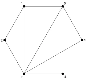
Example 1. LetCbe a 6×6incomplete pairwise comparison matrix as follows:

C=







1 a12 a13 ∗ ∗ a16

a21 1 a23 ∗ ∗ ∗

a31 a32 1 a34 a35 a36

∗ ∗ a43 1 ∗ ∗

∗ ∗ a53 ∗ 1 a56

a61 ∗ a63 ∗ a65 1





 .

Then, the corresponding graphs Gand −→G are presented in Figures 1 and 2.

(8)

Figure 1. The undirected graph Gcorresponding to matrix C

Figure 2. The directed graph −→G corresponding to matrix C

Remark 1. In the case of a complete matrix, G is the complete undirected graph ofn vertices and−→G is the complete directed graph ofn vertices, the edges of which are oriented in both ways and loops are added at the vertices.

(9)

3 The eigenvector method for incomplete ma- trices

In this section, the eigenvalue optimization problem (4) is discussed. Starting from an incomplete pairwise comparison matrix in form (6), we show that problem (4) can be transformed into a convex optimization problem, moreover, under a natural condition, into a strictly convex optimization problem.

This latter statement is our main result here.

Let us parameterize the entries of the (complete or incomplete) pairwise comparison matrix A(x) = A(x₁, x₂, . . . , xd) of form (6) as xi =e^yⁱ, (i= 1,2, . . . , d). This way we obtain a matrix

A(x) =B(y) =B(y1, y2, . . . , yd). (7) Definition 1. LetC ⊆R^k be a convex set and f :C →R+. A function f is called logconvex (or superconvex), iflogf :C→R is a convex function.

It is easy to see that a logconvex function is convex as well.

Proposition 1. For the parametrized matrix B(y) from (7) the Perron eigenvalue λmax(B(y)) is a logconvex (hence convex) function of y.

Proposition 1 has been proved by Aupetit and Genest [2], for the case when d= 1.The proof is based on Kingman’s theorem as follows.

Theorem 1. (Kingman [18]): If the elements of matrix A ∈ R^n×n, denoted by aij(t), (i, j = 1,2, . . . , n) are logconvex functions of t, then λmax(A(t))is logconvex (hence convex).

Proposition 1 for general d can also be proved by applying Theorem 1.

It is enough to show the logconvexity along the lines in the space y. The pairwise comparison matrices along any line in the yspace can be written as

B(t) =

e^c^ij^t+d^ij

i,j=1,...,n, (8)

wheretis a scalar variable, andcij, dij ∈R.Note that a matrix of this form is a pairwise comparison matrix for every value of t if and only if cii =dii = 0;

and cij =−cji, dij =−dji hold for every i, j.

Note also, that if the value aij is known, then we have cij = 0, and dij =

(10)

logaij. Using the parametrization of the line, Proposition 1 follows immediately from Theorem 1. However, for the reader’s convenience, and since some ideas of the proof will be used later, we outline a simple direct proof of Proposition 1.

Proof of Proposition 1: It suffices to show logconvexity along lines in the y space. It is sufficient to prove that λmax(B(t))is a logconvex function of the real variable t.

It is known (see, e.g., in [15], take the trace in Theorem 8.2.8) that for a strictly positive matrix A one has

λmax(A) = lim

m→∞

mp

T r(A^m).

Write

f(t) =fm(t) =T r((B(t))^m).

It suffices to prove that fm(t) is a logconvex function of t. Indeed, then

1

mlogfm(t)is convex, hence the limit,logλmax(t)is convex [25]. Here we use also the fact, that λmax≥n [26], hencefm(t) can be bounded away from 0.

It remains to verify that f(t) = fm(t) is logconvex. From the definition of the parametrization (8) we see that

f(t) = XN

i=1

e^cⁱ^t+dⁱ,

where N is a positive integer and ci, di ∈R (i, j = 1,2, . . . , N), all depend also on m. We have to prove thatlogf(t) is convex.

Lemma 1. The function f(t) above is logconvex.

Proof of Lemma 1: The convexity of logf(t)is to be proved.

[logf(t)]^′ = f^′(t) f(t)

[logf(t)]^′′ = f^′′(t)f(t)−f^′(t)f^′(t) f²(t)

It is enough to prove the non-negativity of the numerator, that is, the inequality f^′′(t)f(t)−f^′(t)f^′(t)≥0.

Since

f^′(t) = XN

i=1

cie^cⁱ^t+dⁱ,

(11)

f^′′(t) = XN

i=1

c²_ie^cⁱ^t+dⁱ,

we have

XN

i=1

c²_ie^cⁱ^t+dⁱ

! _N X

i=1

e^cⁱ^t+dⁱ

!

− XN

i=1

cie^cⁱ^t+dⁱ

!2

= X

i6=j

(c²_i +c²_j −2cicj)e^(cⁱ^+c^j^)t+dⁱ^+d^j ≥0,

which completes the proof of Lemma 1 as well as of Proposition 1.

Corollary 1. The tools of convex optimization can be used for solving the eigenvalue minimization problem (4).

Proposition 2: λmax(B(y)) is either strictly convex or constant along any line in the y space.

Proof of Proposition 2: Consider the parametrization of a line in the y space according to (8) and let

g(t) = λmax(B(t)), t∈R.

The functiong is logconvex and we shall show that it is either strictly convex or constant.

Assume that g is not strictly convex. Then there exist t1, t2 ∈R, t1 < t2 and 0< κ0 <1such that

g(κ0t1+ (1−κ0)t2) =κ0g(t1) + (1−κ0)g(t2). (9) Since the logarithmic function is strictly concave, we get from (9) that

logg(κ₀t₁+ (1−κ₀)t₂) = log(κ₀g(t₁) + (1−κ₀)g(t₂))≥

≥κ0logg(t1) + (1−κ0) logg(t2), (10) furthermore, the inequality in (10) holds as an equality if and only if g(t1) =g(t2). On the other hand, from the logconvexity of g we have

logg(κ₀t₁+ (1−κ₀)t₂)≤κ₀logg(t₁) + (1−κ₀) logg(t₂), (11) Now, (10) and (11) imply that g(t1) =g(t2)and taking (9) also into consideration:

g(κ₀t₁+ (1−κ₀)t₂) =g(t₁) =g(t₂).

(12)

Since g is convex, g(t)is constant on the interval [t1, t2]. Let Λ =g(t1).

Then Λ is the minimal value of g over the real line R.Let

S ={t∈R|g(t) = Λ}. (12)

Clearly [t1, t2] ⊆S, S is a convex and close subset of R, furthermore, since t1 < t2, S has a nonempty interior.

If S = R, we are done. Otherwise, we have either max{t|t ∈ S} < ∞ or min{t|t∈ S}>−∞. It suffices to detail the proof for one of these cases.

Assume that

t= max{t|t∈S}<∞. SinceΛ =g(t) =λmax(B(t)), ∀t∈S, we have

det(B(t)−ΛI) = 0, ∀t ∈S. (13) From the parametrization (8), we obtain

det(B(t)−ΛI) =α0+ XL

l=1

αle^β^l^t, (14)

where the values ofLand αl, βl come from the expansion of the determinant, and they depend on B(t)and Λ.Let

p(t) = α0+ XL

l=1

αle^β^l^t.

p(t) is an analytical function, which equals to zero on a segment [t₁, t₂]. By the Identity Theorem for complex analytic functions (Theorem 1.3.7 in Ash [1]) we have p(t) = det(B(t)−ΛI) = 0for allt∈R. This means thatΛ is an eigenvalue of B(t) for all t∈R. However, due to the properties that Perron eigenvalue of a positive matrix has multiplicity 1 (see Theorem 37.3 in [24]) and that the eigenvalues change continuously witht even when multiplicities are taken into consideration (see for example Rouché’s Theorem in [1]), it cannot happen thatΛ is the Perron eigenvalue in t =t, but it is not for any t > t. Consequently, we cannot have t <∞, thus S =R and

g(t) =λmax(B(t)) = Λ

(13)

for all t∈R. This completes the proof of Proposition 2.

The main result of this section is the following uniqueness theorem.

Theorem 2: The optimal solution of problem (4) is unique if and only if the graph G corresponding to the incomplete pairwise comparison matrix is connected.

Proof of Theorem 2: Necessity is based on elementary linear algebra.

If G is not connected, then the incomplete pairwise comparison matrix A can be rearranged by simultaneous changes of the rows and the columns into a decomposable form D:

D=







J X X^′ K





, (15)

where the square matrices J,Kcontain all the known elements of the incomplete pairwise comparison matrix A and X contains variables only. Matrix X^′ contains the componentwise reciprocals of the variables in X. Note that matrices J,K may also contain variables.

Assume that J is a u×u matrix. Let α > 0 be an arbitrary scalar and P = diag(α, α, . . . , α

| {z }

u

,1,1, . . . ,1

| {z }

n−u

). Then, the similarity transformation by P results in the matrix

PDP⁻¹ =E=







J α·(X)

1

α ·(X^′) K





,

For any fixed values of the variables in X the matrices A, D and E are similar. Since α > 0 is arbitrary, one may construct an infinite number of completions of A having the same eigenvalues, including the largest one.

For sufficiency, the directed graph representation introduced in Section 2 is considered.

We call a sequence of integers i₀, i₁, . . . , i_k−1, i₀ a closed walk of length k, provided that 0< ij ≤n holds forj = 0, . . . , k−1.

Let A = [aij] be an n×n matrix and γ = i0, i1, . . . , ik−1, i0 be a closed walk. The value vγ of γ is defined as the product of the entries of A along

(14)

the walk:

vγ :=ai0i1ai1i2· · ·ai_k−1i0.

Lemma 2. Let A = [aij] be a strictly positive n × n matrix and γ =i0, i1, . . . ik−1, i0 be a closed walk of length k. Then λmax(A)≥(vγ)^k¹.

Proof of Lemma 2: The formula λmax(A) = lim

m→∞

mp

T r(A^m) is used again.

Set m=ℓk, where ℓ is a positive integer. ThenT r(A^m) =P

δvδ, where the summation is for all the n^m closed walks δ of length m. The terms of the sum are positive by assumption. Let δ^∗ be the walk obtained by passing throughγ exactly ℓ times. Nowδ^∗ is a closed walk of lengthm andvδ^∗ =v_γ^ℓ. We infer that

mp

T r(A^m)> ^m√vδ^∗ = ^ℓkq

v_γ^ℓ = √^kvγ. The claim follows by taking ℓ → ∞.Lemma 2 is proved.

Lemma 3. Let the graph Gof the incomplete pairwise comparison ma- trixAbe connected. Let xh, (1≤h≤d)be one of the missing elements and (l, m) denote the position ofxh in the matrix. Then

λmax(A(x)) ≥max (

(Kxh)¹^k, 1

Kxh

¹_k) ,

where k >1is an integer, K >0, and the values of k andK depend only on the known elements of the matrix and on l, m, but not on the value of xh.

Proof of Lemma 3: Since G in connected, for some k there exists a path l = i0, i1, . . . , ik−1 = m in G connecting l to m. Please note that the entries airi_r+1 are all specified values inA for r = 0, . . . , k −1. Let γ be the following closed walk of length k

γ :=i0, i1, . . . , ik−1, i0. By Lemma 2 we have

λmax(A(x))≥(vγ)¹^k = (K·xh)¹^k,

where K = ai0i1ai1i2· · ·ai_k−2i_k−1 is a positive constant independent of the specializations of the variables xi, (i= 1,2, . . . , d). We obtain

λmax(A(x))≥ 1

Kxh

¹_k

(15)

in a similar way, simply taking the reverse direction of the closed walk γ.

Lemma 3 is proved.

Now we turn to the proof of Theorem 2. We are interested in Λ :=

minλmax(A), where the minimum is taken over all (numerical) reciprocal matrices which are specializations of A. To put it simply, we write positive real numbers bij in the place of the variables xh(h = 1,2, . . . , d) in all possible ways while maintaining the relations bijbji = 1, and take the minimum of the Perron roots of the reciprocal matrices obtained.

As before, we introduce the parametrization

x1 =e^y¹, x2 =e^y², . . . xd =e^y^d. (16) This wayA(x) = B(y)is parameterized by vectorsy= (y1, . . . , yd)from the space R^d. Set

Λ := min{λmax(B(y)) : y∈R^d}, (17) and

S ={y∈R^d: λmax(B(y)) = Λ}. (18) It follows from the connectedness of the graph G that the minimum is indeed attained in the definition ofΛ.Assume for contradiction, that infimum exists only, then there is a sequence of vectors inR^d,denoted by{y⁽ⁱ⁾}^i=1,...,∞, such that

i→∞limλmax(B(y⁽ⁱ⁾)) = Λ and

sup{y_h⁽ⁱ⁾}^i=1,...,∞ =∞, (19)

or

inf{y_h⁽ⁱ⁾}^i=1,...,∞=−∞. (20)

for some h(1 ≤ h ≤ d). It follows from reciprocal property of pairwise comparison matrices that (19) and (20) are practically equivalent, therefore, it is sufficient to discuss (19). After possibly renaming we may assume that

i→∞limy_h⁽ⁱ⁾=∞,

which contradicts Lemma 3 by choosing x⁽ⁱ⁾_h =e^y⁽ⁱ⁾^h , since Λ is a fixed finite number.

We shall prove that if |S|> 1, then the graph G of A is not connected.

To this end, assume first that p,q∈R^d are two different points ofS. Let L

(16)

be the line passing throughpandq.It follows from Proposition 2 thatL⊆S.

From L ⊆ S we obtain that there exists an undefined position (l, m) in the upper triangular part of matrix A, such that for every real M > 0there exists a completion C= [cij] of A (a complete pairwise comparison matrix, which agrees with A everywhere, where aij has been specified), such that λmax(C) = Λ and clm > M. It contradicts to Lemma 3 by setting xh =clm, because then λmax(C) will be unbounded if clm is arbitrarily large. This completes the proof of Theorem 2.

Corollary 3. If the graph G corresponding to the incomplete pairwise comparison matrix is connected, then by using the parametrization (16), problem (4) is transformed into a strictly convex optimization problem. Moreover, taking λmax(A(x))at an arbitrary x>0 as an upper bound of the optimal value of (4), a positive lower and an upper bound can be immediately obtained for xh,(1≤h≤d)from Lemma 3. This makes it possible to search for the optimal solution of (4) (and (17)) over ad-dimensional rectangle. We propose an algorithm for solving (4) in Section 5.

Consider the graph Gcorresponding to the incomplete pairwise comparison matrix A. A subgraph G^′ of G is called a connected component of G if it is a maximal connected subgraph of G. Clearly, G can be divided into a finite number of disjoint connected components. Let G1, . . . , Gs denote the connected components of G. The graph Gis connected when s = 1. In this case, according to Theorem 2, the optimal solution of problem (4) (thus of (17)) is unique. The next theorem extends this result to the general case, namely, proves that the minimum of (4) (equivalently Λ of (17)) exists and characterizes the set of the optimal solutions, i.e. S of (18) in they space.

Theorem 3: The functionλmax(B(y))attains its minimum overR^d, and the optimal solutions constitute an(s−1)-dimensional affine set ofR^d, where s is the number of the connected components in G.

Proof of Theorem 3: If s= 1, we are done. By Theorem 2, there is a single optimal solution, and itself is a 0-dimensional affine set.

We turn now to the case s >1. First, we show that λmax(B(y)) attains its minimum over R^d. An idea from the proof of Theorem 2 is used here again. For l = 1, . . . , s−1, applying necessary simultaneous changes of the rows and the columns, the incomplete pairwise comparison matrix Acan be rearranged into the decomposable form D of (15) such that the rows and

(17)

the columns ofJ are associated with the nodes of the connected components G1, . . . , Gl, the rows and the columns of K are associated with the nodes of the connected components Gl+1, . . . , Gs, and X consists of the variables whose rows and columns are associated with the nodes of G1, . . . , Gl and Gl+1, . . . , Gs, respectively. Here again, X^′ consists of the reciprocals of the variables inX.

As shown in the proof of Theorem 2, for any x ∈ R^d+, the value of λmax(A(x)) does not change if all the entries of x belonging to the block X in (15) are multiplied by the same α >0. Choose a variable xil from the block X arbitrarily such that its row and column are associated withGl and G_l+1, respectively. We can fix the value of xil at any positive level, say let xil = vil. Then, for any x ∈ R^d+ the vector ¯x ∈ R^d+ obtained from x by multiplying all the entries from the blockXby α=vi_l/xi_l has the properties

¯

xil =vil and λmax(A(¯x)) =λmax(A(x)).

Repeat the above idea for l = 1, . . . , s−1. In this way, we can choose variables xi_l, l = 1, . . . , s−1, such that they belong to missing elements of A, the row and column ofxil are associated with Gl and Gl+1, respectively;

furthermore, for anyx∈R^d+and for fixed valuesvil, l= 1, . . . , s−1, a vector

¯

x ∈ R^d+ can be easily constructed such that x¯i_l =vi_l, l = 1, . . . , s−1, and λmax(A(¯x)) =λmax(A(x)).

Thus, if we are interested only in finding an optimal solution of (4), it suffices to write arbitrary positive values into those missing entries of matrix A which belong to xi1, . . . , xis−1, and of course, the reciprocal values into the appropriate entries in the lower triangular part of A. Let A˜ denote the pairwise comparison matrix obtained in this way. Matrix A˜ has d−s+ 1 missing entries in the upper triangular part, and the graphGassociated with A˜ is connected. Thus, the problem

min˜x>0λmax(A(˜˜ x)) (21) has a unique optimal solution, where x˜ is the(d−s+ 1)-dimensional vector associated with the missing entries in the upper triangular part of A. It is˜ easy to see that by completing the optimal solution of (21) by the entries xi₁, . . . , xi_s−1 fixed inA, we obtain an optimal solution of (4), moreover, due to (16), an optimal solution where λmax(B(y)) attains its minimum overR^d, i.e. Λ of (17) exists andS of (18) is not empty.

We know that |S| > 1 if and only if s > 1. Let y,¯ ˆy ∈ S, y¯ 6= y.ˆ Since λmax(B(¯y)) = λmax(B(ˆy)) = Λ, we have λmax(B(y)) = Λ along the entire line passing through y¯ and ˆy. This comes from Proposition 2 since if λmax(B(y)) was strictly convex along the line, we would haveλmax(B(y))<

Λ for any interior point of the segment [¯y,ˆy]contradicting the minimality of

(18)

Λ. Consequently, for any ¯y,ˆy∈S, ¯y6=ˆy, the line passing through y¯ and yˆ lies in S, thus S is an affine set in the y space.

The affine set S can be written in the form of the solution set of a finite system of linear equalities

Fy=f, (22)

see [25]. For the sake of simplicity, assume that il = l, l = 1, . . . , s− 1, and for any y ∈ R^d, let y⁽¹⁾ be the vector of the first s −1 elements, and let y⁽²⁾ be the vector of the last d − s + 1 elements of y, i.e. y = (y⁽¹⁾^T,y⁽²⁾^T)^T. We know that for anyy⁽¹⁾there exists a uniquey⁽²⁾ such that y= (y⁽¹⁾^T,y⁽²⁾^T)^T ∈S. Lety⁽²⁾ =h(y⁽¹⁾)denote this relation. Since for any

¯

y⁽¹⁾,yˆ⁽¹⁾ ∈R^s−1 and α∈R, the vectors (¯y⁽¹⁾^T, h(¯y⁽¹⁾)^T)^T,(ˆy⁽¹⁾^T, h(ˆy⁽¹⁾)^T)^T and ((α¯y⁽¹⁾+ (1−α)ˆy⁽¹⁾)^T,(αh(¯y⁽¹⁾) + (1−α)h(ˆy⁽¹⁾))^T)^T are solutions of (22), we obtain that

h(α¯y⁽¹⁾+ (1−α)ˆy⁽¹⁾) =αh(y¯⁽¹⁾) + (1−α)h(yˆ⁽¹⁾),

i.e. h is a linear function. Let e^(l) denote the l-th unit vector. It is easy to see that the s vectors (0^T, h(0)^T)^T, (e^(l)T, h(e^(l))^T)^T, l = 1, . . . , s−1, are affinely independent, and their affine hull is the solution set of (22), i.e. S.

Consequently, S is a(s−1)-dimensional affine set, see [25]. This completes the proof of Theorem 3.

Corollary 4. It follows from Theorem 3 that if we are interested only in finding an optimal solution of (4), it suffices to solve (21) that can be, as shown before, reduced to the minimization of a strictly convex function over a rectangle. If we are interested in generating the whole set S, the proof of Theorem 3 shows how to construct affinely independent vectors whose affine hull is S.

Althoughλmax(A(x))is non-convex over R^d+ it is either constant or uni- modal over any line parallel to an axis, i.e., when a single entry of the pairwise comparison matrix varies. This comes directly from Proposition 2 and the parametrization (16). The advantage of this property will be used in Section 5 when the method of cyclic coordinates will be applied for solving (4).

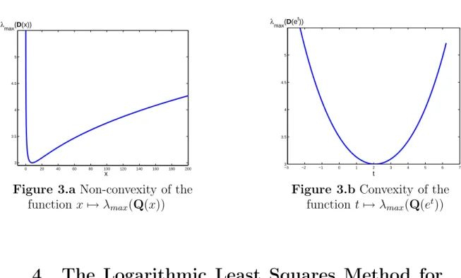
Remark 2. The Perron eigenvalue of a pairwise comparison matrix is non-convex function of its elements. Let Q be a 3×3 pairwise comparison matrix of variable x as follows:

Q=





1 2 x

1/2 1 4 1/x 1/4 1



.

(19)

λmax(Q(x)) is plotted in Figure 3.a. However, by using the exponential scaling x=e^t, λmax(Q(e^t)) becomes a convex function oft (Figure 3.b).

0 20 40 60 80 100 120 140 160 180 200

3 3.5 4 4.5 5

x λ_max(D(x))

Figure 3.a Non-convexity of the function x7→λmax(Q(x))

−3 −2 −1 0 1 2 3 4 5 6 7

3 3.5 4 4.5 5

t λ_max(D(e^t))

Figure 3.b Convexity of the functiont 7→λmax(Q(e^t))

4 The Logarithmic Least Squares Method for incomplete matrices

In this section, the extension of the LLSM problem (3) for incomplete matrices is discussed. Having an incomplete pairwise comparison matrixA,one should consider the terms for those pairs (i, j) only for which aij is given:

min X

e(i, j)∈E 1≤i < j≤n

logaij −log wi

wj

2

+

logaji−log wj

wi

2

(23)

Xn

i=1

wi = 1, (24)

wi >0, i= 1,2, . . . , n. (25)

For the reader’s convenience, each pair of terms related to aij and aji is written jointly in the objective function (23). By definition, the terms related to i=j equal to 0, therefore, they are omitted from the objective function.

(20)

Theorem 4: The optimal solution of the incomplete LLSM problem (23)-(25) is unique if and only if graph G corresponding to the incomplete pairwise comparison matrix is connected.

Proof: Since the value of the objective function is the same in an arbitrary point wand in αw for any α >0we can assume that

wn = 1, (26)

instead of normalization (24). Following Kwiesielewicz’s computations for complete matrices [20](pp. 612-613), let us introduce the variables

rij = logaij i, j = 1,2, . . . , nand e(i, j)∈E; (27) yi = logwi i= 1,2, . . . , n. (28) Note that yn = logwn = 0. The new problem, equivalent to the original one, is as follows:

min X

i, j: e(i, j)∈E 1≤i < j < n

(rij −yi+yj)²+ X

i: e(i, n)∈E

(rin−yi)² (29)

This problem is unconstrained (y1, y2, . . . , yn−1 ∈ R). The first-order conditions of optimality can be written as:







d₁ −1 0 . . . −1

−1 d2 −1 . . . 0 0 −1 d3 . . . 0 ... ... ... ... ...

−1 0 0 . . . dn−1











 y₁ y2

y3

...

yn−1







=







−P r_i1

−P ri2

−P ri3

...

−P ri,n−1







, (30)

where di denotes the degree of the i-th node in graph G (0 < di ≤ n−1), and the (i, j) position equals to −1 if e(i, j) ∈ E and 0 if e(i, j) ∈/ E. Note that the summation P

rik denotes X

i: e(i, k)∈E

rik

in each component (k = 1,2, . . . , n−1) of the right-hand side.

(21)

The matrix of the coefficients of size(n−1)×(n−1)can be augmented by then-th row and column based on the same rules as above: (n, n)position equals to dn, the degree of n-th node in graph G; (i, n) and (n, i) positions equal to −1 if e(i, n) ∈E (or, equivalently, e(n, i) ∈E) and 0 if e(i, n) ∈/ E (or, equivalently, e(n, i) ∈/ E) for all i = 1,2, . . . , n−1. The augmented n×n matrix has the same rank as the(n−1)×(n−1)matrix of the coefficients in (30) because the number of−1’s in thei-th row/column is equal to di(i = 1,2, . . . , n) and the n-th column/row is the negative sum of the first n−1columns/rows.

Now, the augmented matrix of size n×n, is exactly the Laplace-matrix of graph G, denoted by L_n×n. Some of the important properties of Laplace- matrix L_n×n are as follows (see, e.g., Section 6.5.6 in [11]):

(a) eigenvalues are real and non-negative;

(b) the smallest eigenvalue,λ1 = 0;

(c) the second smallest eigenvalue, λ2 >0 if and only if the graph is connected; λ2 is called Laplace-eigenvalue of the graph;

(d) rank ofL_n×n is n−1 if and only if graph Gis connected.

LetL(n−1)×(n−1) denote the upper-left(n−1)×(n−1)submatrix ofL_n×n. The solution of the system of first-order conditions uniquely exists if and only if matrix L(n−1)×(n−1) is of full rank, that is, graph Gis connected.

Since the equations of the first-order conditions are linear, the Hessian matrix is again L(n−1)×(n−1), which is always symmetric, and, following from the properties of Laplace-matrix above, it is positive definite if and only if graph G is connected.

Remark 3. The uniqueness of the solution depends only on the positions of comparisons (the structure of the graph G), and does not depend on the values of comparisons.

Remark 4. In the case of ann×ncomplete pairwise comparison matrix, the solution of (30) is as follows:





 y1

y2

y₃ ...

yn−1







=







n−1 −1 −1 . . . −1

−1 n−1 −1 . . . −1

−1 −1 n−1 . . . −1 ... ... ... ... ...

−1 −1 −1 . . . n−1







−1





−P ri1

−P ri2

−P r_i3 ...

−P ri,n−1







, (31)

(22)

whereP

rik consists ofn−1elements for everyk(1≤k≤n−1)and equals to the logarithm of the product of the k-th row’s elements of the complete pairwise comparison matrix. Applying (28) and (26), then renormalizing the weight vector by (24), the optimal solution of (23)-(25) is the well known geometric mean, also mentioned in the introduction (3).

Remark 5. Problem (29) has some similarities with additive models of pairwise comparisons, e.g., with the constraints in Xu’s goal programming model [33](LOP1 on p. 264). However, Xu’s objective function is linear, while (29) is quadratic. Fedrizzi and Giove considers several penalty functions originated from equations for consistency. One of their models [9]((4) on p. 304) is also similar, but not equivalent, to our (29).

Remark 6. Theorem 4 shows similarity to Theorem 1 of Fedrizzi and Giove [9](p. 310) regarding the uniqueness of the optimal solution and the connectedness of graph G. In both problems a sum of quadratic functions associated with the edges of G is minimized, although the functions are different in the two approaches.

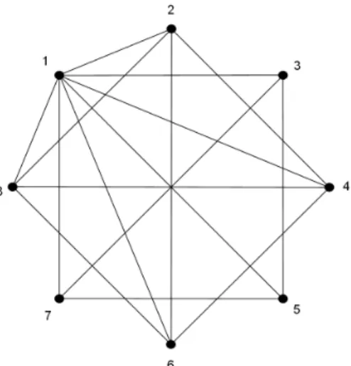
Example 2. As an illustration to the incomplete LLSM problem and our proposed solution, we introduce the partial matrix M below. In fact, M is an incomplete modification of the frequently cited ’Buying a house’

example by Saaty [27]. The undirected graph representation of the partial matrix M in shown in Figure 4.

M=







1 5 3 7 6 6 1/3 1/4

1/5 1 ∗ 5 ∗ 3 ∗ 1/7

1/3 ∗ 1 ∗ 3 ∗ 6 ∗

1/7 1/5 ∗ 1 ∗ 1/4 ∗ 1/8

1/6 ∗ 1/3 ∗ 1 ∗ 1/5 ∗

1/6 1/3 ∗ 4 ∗ 1 ∗ 1/6

3 ∗ 1/6 ∗ 5 ∗ 1 ∗

4 7 ∗ 8 ∗ 6 ∗ 1







. (32)

(23)

Figure 4. The undirected graph representation of the 8×8incomplete pairwise comparison matrix M

Using the notation of (27), the system of linear equations (30) is as follows:







7 −1 −1 −1 −1 −1 −1

−1 4 0 −1 0 −1 0

−1 0 3 0 −1 0 −1

−1 −1 0 4 0 −1 0

−1 0 −1 0 3 0 −1

−1 −1 0 −1 0 4 0

−1 0 −1 0 −1 0 3











 y1

y2

y3

y4

y5

y6

y7







=







−log(1/315)

−log(7/3)

−log(1/6)

−log 1120

−log 90

−log 27

−log(2/5)







, (33)

where thek-th (k = 1,2, . . . ,7) component of the right-hand side is computed as the negative sum of the logarithms of thek-th column’s elements in matrix Min (32), which also equals to the logarithm of the product of thek-th row’s elements.

The solution of (33) is y1 = −0.6485, y2 = −1.6101, y3 = −0.6485, y₄ =−2.8449, y₅ =−2.2214, y₆ =−2.0998, y₇ =−0.8674.

Using (28), then turning back to the normalization (24), the optimal solution of the incompleteLLSMproblem concerning matrixMis as follows:

w^LLSM₁ = 0.1770, w^LLSM₂ = 0.0676, w₃^LLSM = 0.1770, w₄^LLSM = 0.0197, w^LLSM₅ = 0.0367, w^LLSM₆ = 0.0415, w₇^LLSM = 0.1422, w₈^LLSM = 0.3385.

(24)

5 An algorithm for the λ

max

-optimal comple- tion

In this section, an algorithm is proposed for finding the best completion of an incomplete pairwise comparison matrix by the generalization of the eigenvector method. It is shown in Section 3 that the eigenvalue minimization leads to a convex optimization problem. However, the derivatives of λmax as functions of missing elements are not easily and explicitly computable. Therefore, one should provide an algorithm without derivatives. In our approach, the iterative method of cyclic coordinates is proposed. Let d denote the number of missing elements. Write variables x1, x2, . . . , xd in place of the missing elements. Let x⁽⁰⁾_i , i= 1,2, . . . , d be arbitrary positive numbers, we will use them as initial values. Each iteration of the algorithm consists of d steps.

In the first step of the first iteration, let variablex1 be free and the other variables be fixed to the initial values: xi = x⁽⁰⁾_i , (i = 2,3, . . . , d). The aim is to minimize λmax as a univariate function of x1. Since the eigenvalue optimization can be transformed into a multivariate convex optimization problem, it remains convex when restricting to one variable. Let x⁽¹⁾₁ denote the optimal solution computed by a univariate minimization algorithm.

In the second step of the first iterationx2 is free, the other variables are fixed as follows: x1 =x⁽¹⁾₁ , xi =x⁽⁰⁾_i , (i= 3,4, . . . , d).. Now we minimize λmax in x2. Let x⁽¹⁾₂ denote the optimal solution.

After analogous steps, the d-th step of the first iteration is to minimize λmax in xd, where all other variables are fixed by the rule xi = x⁽¹⁾_i , (i = 1,2, . . . , d−1).The optimal solution is denoted byx⁽¹⁾_d and it completes the first iteration of the algorithm.

In the second iteration the initial values computed in the first iteration are used. The univariate minimization problems are analogously written and solved.

The stopping criteria can be modified or adjusted in different ways. In our tests accuracy is set for 4 digits. The algorithm stops in the end of the k-th iteration if k is the smallest integer for which max

i=1,2,...,dkx^k_i −x^k−1_i k< T, where T denotes the tolerance level.

The global convergence of cyclic coordinates is stated and proved, e.g., in ([22], pages 253-254).

In our tests, x⁽⁰⁾_i = 1, (i = 1,2, . . . , d) and T = 10⁻⁴ were applied. We

(25)

used the function fminbnd in Matlab v.6.5 for solving univariable minimization problems.

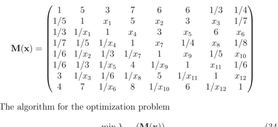
For the reader’s convenience, our algorithm is presented on the 8 ×8 incomplete pairwise comparison matrix M from the previous section (32).

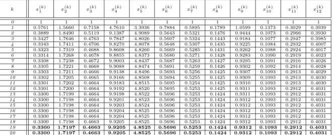
The aim is to find the completion ofM for which λmax is minimal. Write the variables xi, (i = 1,2, . . . ,12; xi ∈ R+) in place of the missing elements and let x= (x₁, x₂, x₃, x₄, x₅, x₆, x₇, x₈, x₉, x₁₀, x₁₁, x₁₂).

M(x) =







1 5 3 7 6 6 1/3 1/4

1/5 1 x₁ 5 x₂ 3 x₃ 1/7

1/3 1/x1 1 x4 3 x5 6 x6

1/7 1/5 1/x4 1 x7 1/4 x8 1/8 1/6 1/x₂ 1/3 1/x₇ 1 x₉ 1/5 x₁₀ 1/6 1/3 1/x5 4 1/x9 1 x11 1/6

3 1/x3 1/6 1/x8 5 1/x11 1 x12

4 7 1/x6 8 1/x10 6 1/x12 1







The algorithm for the optimization problem

minx λmax(M(x)) (34)

is as follows. Let x^(k)_i denote the value of xi in thek-th step of the iteration, which has 12 substeps for each k.

For k = 0 :

Let the initial points be equal to 1 for every variable:

x⁽⁰⁾_i := 1 (i= 1,2, . . . ,12).

while max

i=1,2,...,12kx^k_i −x^k−1_i k> T x^(k)_i := arg min

xi

λmax(M(x^(k)₁ , . . . , x^(k)_i−1, xi, x^(k−1)_i+1 , . . . , x^(k−1)₁₂ )), i= 1,2, . . . ,12 next k

end while

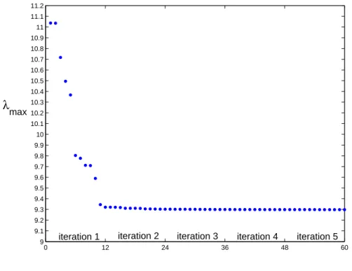
Table 1 presents the results of each substep of the first 20 iterations of the algorithm. Results reach the accuracy up to 4 digits in the 19-th iteration.

After plotting the objective function’s value during the iteration steps, it may be observed, that a significant decrease happens in the first iteration (Figure 5).