On Saaty's and Koczkodaj's inconsistencies of pairwise comparison matrices

(1)

On Saaty ’s and Koczkodaj ’s inconsistencies of pairwise comparison matrices

¹

Bozóki, S. and Rapcsák, T.

Computer and Automation Research Institute, Hungarian Academy of Sciences,

Budapest, Hungary

Abstract

The aim of the paper is to obtain some theoretical and numerical properties of Saaty’s and Koczkodaj’s inconsistencies of pairwise comparison matrices (PRM).

In the case of 3×3 PRM, a differentiable one-to-one correspondence is given be- tween Saaty’s inconsistency ratio and Koczkodaj’s inconsistency index based on the elements of PRM. In order to make a comparison of Saaty’s and Koczkodaj’s inconsistencies for 4×4 pairwise comparison matrices, the average value of the maximal eigenvalues of randomly generated n×n PRM is formulated, the ele- mentsa_ij (i < j) of which were randomly chosen from the ratio scale

1

M, 1

M−1, . . . ,1

2,1,2, . . . , M −1, M,

with equal probability1/(2M−1)anda_jiis defined as1/a_ij. By statistical analysis, the empirical distributions of the maximal eigenvalues of the PRM depending on the dimension number are obtained. As the dimension number increases, the shape of distributions gets similar to that of the normal ones. Finally, the inconsistency of asymmetry is dealt with, showing a different type of inconsistency.

1. Introduction

In multiattribute decision making (MADM), the aim is to rank a finite number of alternatives with respect to a finite number of attributes. Tender evaluations, public pro- curement processes, selections of applicants for positions, decisions on the best portfolios in investments are real-life decision situations in which MADM models can be used.

In solving a multiattribute decision problem, one needs to know the impor- tances or weights of the not equally important attributes and also the evaluations of the alternatives with respect to the attributes. One technique, often used, is the method of pairwise comparisons a concept which is more than two hundred years old.

Condorcet (1785) and Borda (1781) introduced it for voting problems in the 1780’s by using only 0 and 1 in the pairwise comparison matrices. In experimental psychology, Thorndike (1920) and Thurstone (1927) used it in the 1920’s. Especially, pairwise comparisons based on a ratio scale is one of the basic pillars of theAnalytic Hierarchy Process (Saaty, 1980).

1This research was supported, in part, by the Hungarian Scientific Research Fund, Grant Nos.

Manuscript of / please cite as

Bozóki, S., Rapcsák, T. [2008]: On Saaty's and Koczkodaj's inconsistencies of pairwise comparison matrices, Journal of Global Optimization, 42(2), pp.157-175. DOI 10.1007/s10898-007-9236-z

http://www.springerlink.com/content/v2x539n054112451

(2)

Givennobjects, e.g., attributes or alternatives, we suppose that the decision maker(s) is (are) able to compare any two of them. In preference modelling, this assumption is called comparability. For any pairs (i, j), i, j = 1,2, . . . , n, the decision maker is requested to tell how many times the i-th object is preferred (or more important) than the j-th one, which result is denoted bya_ij.

By definition,

a_ij >0; (1.1)

aii= 1; (1.2)

a_ij = 1

a_ji, (1.3)

for any pair of indices (i, j), i, j = 1,2, . . . , n. The name of matrices A = [aij]i,j=1,2,...,n ∈ R^n×n with properties (1.1-1.3) is pairwise comparison matrices or positive reciprocal matrices (PRM).

A pairwise comparison matrix A is consistent if it satisfies the transitivity property

aijajk =aik (1.4)

for any indices (i, j, k), i, j, k = 1,2, . . . , n. Otherwise, A is inconsistent. It was shown by Saaty (1980) that a pairwise comparison matrix is consistent if and only if it is of rank one. When a pairwise comparison matrix A is consistent, the normalized weights computed fromA are unique. Otherwise, an approximation of Aby a consistent matrix (determined by a vector) is needed.

A crucial point of this methodology is to determine the inconsistency of the pairwise comparison matrices. The only widely accepted rule of inconsistency is due to Saaty (1980), but his definition does not meet some important requirements (see Section 2). The aim of the paper is to make some comparison on Saaty’s and Koczkodaj’s inconsistencies of pairwise comparison matrices. The two approaches seem to be completely different, because while Saaty’s inconsistency ratio is an index for the departure from randomness,Koczkodaj’s inconsistency index is related to the departure from consistency with the possibility to locate inconsistency.

In Section 2, the question is how to investigate Saaty’s andKoczkodaj’s inconsistencies. In Section 3, the inconsistency formulas of 3×3pairwise comparison matrices are studied from theoretical and computational points of view. A differentiable one-to-one correspondence is given between Saaty’s and Koczkodaj’s inconsistencies. In Section 4, by using statistical tools, the average value of the maximal eigenvalues of randomly generated n×n PRM is formulated, the elements a_ij (i < j) of which were randomly chosen from the ratio scale 1

M, 1

M −1, . . . , 1

2,1,2, . . . , M −1, M, with equal probability 1/(2M−1)and a_ji is defined as1/a_ij. Then, a comparison ofKoczkodaj’s inconsistency index and Saaty’s inconsistency ratio is given for 4×4 pairwise comparison matrices.

In Section 5, the inconsistency of random pairwise comparison matrices is investigated and by statistical analysis, the empirical distributions of the maximal eigenvalues of the PRM depending on the dimension number are obtained. As the dimension number increases, the shape of distributions gets similar to that of the normal ones. In Section 6, the inconsistency of asymmetry is dealt with, showing a different type of inconsistency.

2

(3)

2. Inconsistency indices

In real-life decision problems, pairwise comparison matrices are rarely consistent.

Nevertheless, decision makers are interested in the level of consistency of the judgements, which somehow expresses the goodness or “harmony” of pairwise comparisons totally, because inconsistent judgements may lead to senseless decisions.

Saaty (1980) proposed the following method for calculating inconsistency. Computing the largest eigenvalue λ_max of A, he has shown that λ_max ≥ n and equals to n if and only if A is consistent. Then, inconsistency index (CI_n) is defined by

CI_n = λ_max−n n−1 ,

which gives the average inconsistency. Mathematically, inconsistency is not but a rescaling of the largest eigenvalue. Since λ_max ≥ n, CI_n is always non-negative. The inconsistency index in its own has no meaning, unless we compare it with some bench- mark to determine the magnitude of the deviation from consistency. Let a set of e.g.,500 random pairwise comparison matrices of size n×n be generated so that each element aij (i < j)be randomly chosen from the scale

1 9,1

8,1

7, . . . ,1

2,1,2, . . . ,8,9, and a_ji is defined as 1

aij

. Let RI_n denote the average value of the randomly obtained inconsistency indices, which depends not only on n but on the method of generating random numbers, too. The inconsistency ratio (CR_n) of a given pairwise comparison matrix A indicating inconsistency is defined by

CRn= CIn

RI_n.

If the matrix is consistent, then λ_max = n, so CI_n = 0 and CR_n = 0, as well.

Saaty concluded that an inconsistency ratio of about 10% or less may be considered acceptable. The intuitive meaning of the 10 percent rule is skipped by several authors.

A statistical interpretation of the 10 percent rule is given by Vargas (1982). More recently, Saaty’s threshold is 5% for 3×3, and 8% for 4×4 matrices (Saaty, 1994).

It is emphasized that the inconsistency ratio CRn is related to Saaty’s scale. The structuring process in AHP specifies that items to be compared should be within one order of magnitude. This helps avoid inaccuracy associated with cognitive overload as well as aijajk relationships that are beyond the 1-9 scale, see e.g. Lane and Verdini (1989) and Murphy (1993). If only two attributes (or alternatives) are present, inconsistency is always zero, since the decision maker gives only one importance ratio.

Though the only one widely accepted rule of inconsistency for any order of matrix is due to Saaty, its consistency definition has some drawbacks. By Koczkodaj (1993),

“The author of this paper truly believes that failure of the pairwise comparison method to become more popular has its roots in the consistency definition.” The major drawback of Saaty’s inconsistency definition seems to be the 10 percent rule of thumb. Another weakness of it is related to the location of inconsistency or rather its lack. Since an eigenvalue is a global characteristic of a matrix, by examining it, we cannot say which matrix element contributed to the increase of inconsistency. Some improvements can be found in Saaty (1990).

(4)

A general 3×3 pairwise comparison matrix has three comparisons a, b, c. In order to defineKoczkodaj’s inconsistency index ¡

Duszak and Koczkodaj (1994) and Koczkodaj (1993)¢

, consider a general 3×3 pairwise comparison matrix. Reduce this reciprocal matrix to a vector of three coordinates (a, b, c). In the consistent cases, the equality b = ac holds. It is always possible to produce three consistent reciprocal matrices (represented by three vectors) by computing one coordinate from the combination of the remaining two coordinates. These three vectors are:

µb c, b, c

¶

,(a, ac, c)and µ

a, b, b a

¶ . The inconsistency index of a general 3×3pairwise comparison matrix is defined by Koczkodaj as the relative distance to the nearest consistent 3×3 pairwise comparison matrix represented by one of these three vectors.

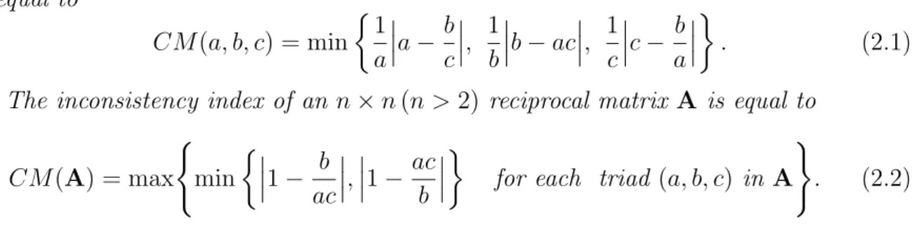
Definition 2.1 The inconsistency index of a general 3×3 pairwise comparison matrix is equal to

CM(a, b, c) = min

½1 a

¯¯

¯a− b c

¯¯

¯, 1 b

¯¯

¯b−ac

¯¯

¯, 1 c

¯¯

¯c− b a

¯¯

¯

¾

. (2.1)

The inconsistency index of an n×n(n >2) reciprocal matrix A is equal to

CM(A) = max (

min

½¯¯¯1− b ac

¯¯

¯,

¯¯

¯1− ac b

¯¯

¯

¾

for each triad (a, b, c) in A )

. (2.2) In the case of matrices of higher orders, the inconsistency index of a matrix element is equal to the maximum of CM of all possible triads which include this element.

Note that the inconsistency index is not a metric. By Duszak and Koczkodaj (1994), the number of all possible triads of the n×n comparison matrices is equal to

n(n−1)(n−2)/3!. (2.3)

In the case of 4×4 pairwise comparison matrices and a scale of 1 to 5, the threshold should be 1/3 (Koczkodaj et al., 1997).

Other inconsistency indices have been introduced. The inverse inconsistency index suggested by Dodd,Donegan and McMaster (1993),Monsuur (1996) applied a transfor- mation of the maximal eigenvalues, Peláez and Lamata (2003) examined all the triples of elements and used the determinant to indicate consistency, furthermore, Stein and Mizzi (2007) obtained the harmonic consistency index. Another type of inconsistency index is the distance from a specific consistent matrix. Chu,Kalaba andSpingarn (1979) used the least squares estimation error, Crawford and Williams (1985) the logarithmic least squares estimation error, furthermore, Aguarón and Moreno-Jiménez (2003) the geometric consistency index for the logarithmic least squares method (the row geometric mean method).

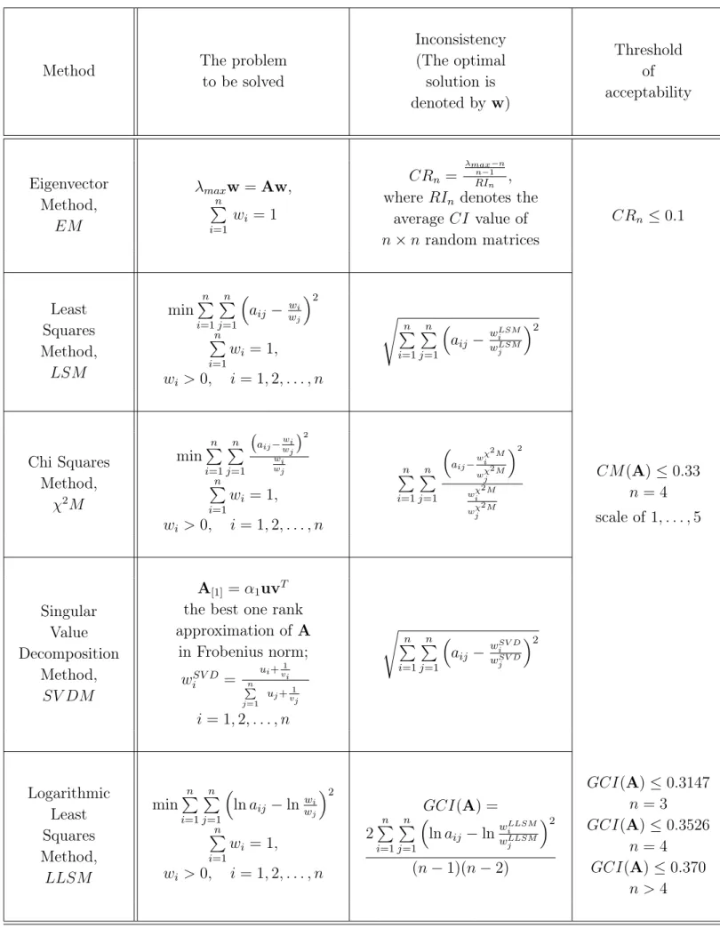
Table 1 summarizes some weighting methods and inconsistency indices, namely, the eigenvector method (EM) and inconsistency ratio (CR) (Saaty, 1980), the least squares method (LSM) (Chu,Kalaba andSpingarn, 1979), theχsquares method (χ²M) (Jensen, 1983), the singular value decomposition method (SVDM) (Gass and Rapcsák, 2004) and Koczkodaj’s inconsistency index (Koczkodaj, 1993, 1994), the logarithmic least squares method (LLSM), (Crawford and Williams, 1985) and GCI,(Aguarón and Moreno-Jiménez, 2003).

4

(5)

Method The problem to be solved

Inconsistency (The optimal

solution is denoted by w)

Threshold of acceptability

Eigenvector Method,

EM

λ_maxw=Aw, Pn

i=1

w_i = 1

CR_n = ^λmax_RIⁿ⁻¹_n⁻ⁿ, where RI_n denotes the

average CI value of n×n random matrices

CR_n≤0.1

Least Squares Method, LSM

minPⁿ

i=1

Pn j=1

³

a_ij − ^w_w_jⁱ

´₂

Pn i=1

w_i = 1,

w_i >0, i= 1,2, . . . , n

sPn

i=1

Pn j=1

³

a_ij − ^w_w^LSMⁱLSM j

´₂

Chi Squares Method,

χ²M

minPⁿ

i=1

Pn j=1

¡

aij−^wi

wj

¢2 wi wj

Pn i=1

wi = 1,

w_i >0, i= 1,2, . . . , n

Pn i=1

Pn j=1

³

aij−^w

χ2M i wχ2M

j

´²

wχ2M i wχ2M

j

CM(A)≤0.33 n = 4 scale of 1, . . . ,5

Singular Value Decomposition

Method, SV DM

A_[1] =α₁uv^T the best one rank approximation of A

in Frobenius norm;

w^{SV D}_i = ^uⁱ⁺

1 n vi

P

j=1

uj+¹

vj

i= 1,2, . . . , n

sPn

i=1

Pn j=1

³

a_ij− ^w_wⁱ^{SV D}SV D j

´₂

Logarithmic Least Squares Method, LLSM

minPⁿ

i=1

Pn j=1

³

lna_ij −ln^w_wⁱ

j

´₂

Pn i=1

wi = 1,

wi >0, i= 1,2, . . . , n

GCI(A) = 2Pⁿ

i=1

Pn j=1

³

lna_ij −ln^w_w^LLSMⁱLLSM j

´₂

(n−1)(n−2)

GCI(A)≤0.3147 n = 3 GCI(A)≤0.3526

n = 4 GCI(A)≤0.370

n >4

Table 1. Weighting methods and inconsistency indices

(6)

3. Inconsistency of 3 × 3 pairwise comparison matrices

In this part, it is shown that there exists a one-to-one correspondence betweenSaaty’s inconsistency ratio and Koczkodaj’s inconsistency index.

The general form of 3×3 positive reciprocal matrices is as follows:





1 a b

1/a 1 c 1/b 1/c 1



, a, b, c∈R+. (3.1)

ByTummalaandLing (1998), the maximal eigenvalues of matrices (3.1) can be explicitly given by the function

λ_max(a, b, c) = 1 + ³ r b

ac+ ³ rac

b , (a, b, c)∈R³₊. (3.2) A consequence of this formula is that λ_max does not change if the elements a and b are multiplied by the same constant. Thus, the CR-inconsistencies of matrices





1 2 2 1 2 1



,





1 7 7 1 2 1



,





1 9 9 1 2 1



 (3.3)

are equal, though the consistency violations in the matrices are different.

By formula (3.2), it is possible to make a connection between λ_max and the inconsistency originated from the elements a, b, cof the positive reciprocal matrices.

Definition 3.1 In the case of (3.1), let T denote the maximum of two ratios, ^ac_b and

b

ac, i.e., T = max©_ac

b ,_ac^bª .

If the matrix is consistent, T equals to 1, otherwise, T >1.

Theorem 3.1In the case of 3×3pairwise comparison matrices, there exists a differen- tiable one-to-one correspondence for every pair of the inconsistency CR defined by Saaty, the inconsistency CM defined by Koczkodaj and T = max©_ac

b,_ac^b ª

as follows:

CR(T) =

√3

T + √3¹

T −2

2RI₃ , T >1. (3.4)

T(CR) = ³

1 +RI₃CR+p

RI₃CR(2 +RI₃CR)´₃

, CR ∈(0,∞), (3.5)

CM(T) = 1− 1

T, T(CM) = 1

1−CM, CM ∈(0,1), (3.6)

CR(CM) =

1

√3

1−CM +√³

1−CM−2

2RI₃ , CM ∈(0,1), (3.7)

CM(CR) = 1− 1

³

1 +RI₃CR+p

RI₃CR(2 +RI₃CR)

´₃, CR∈(0,∞). (3.8)

6

(7)

Proof. From Definition 3.1, it follows that

3

rac b + ³

r b

ac =√³

T + 1

√3

T. Since λmax= 1 + ³

q

ac b + ³

q

b

ac,it can be written in the equivalent form λmax= 1 +√³

T + 1

√3

T. (3.9)

Saaty defined the inconsistency ratio asCR=

λmax−n n−1

RIn . Let us substituten = 3 and (3.9) for the formula ofCR, and (3.4) is proved.

Function CR(T)is differentiable on the domain T > 1, and CR⁰(T) = 1− √₃¹

T²

6RI3 ³

√T², (3.10)

which is positive if T > 1, consequently, CR is invertable in this domain. Its inverse function is equal to

T(CR) =

³

1 +RI₃CR+p

RI₃CR(2 +RI₃CR)

´₃

, CR∈(0,∞), which proves (3.5).

Since

CM = min

½1 a

¯¯

¯a− b c

¯¯

¯, 1 b

¯¯

¯b−ac

¯¯

¯, 1 c

¯¯

¯c− b a

¯¯

¯

¾

=

min

½¯¯¯1− b ac

¯¯

¯,

¯¯

¯1− ac b

¯¯

¯,

¯¯

¯1− b ac

¯¯

¯

¾

= min

½¯¯¯1− b ac

¯¯

¯,

¯¯

¯1−ac b

¯¯

¯

¾ , it follows that

CM(T) = 1− 1

T, CM⁰(T) = 1

T², T > 1, and

T(CM) = 1

1−CM, T⁰(CM) = 1

(1−CM)², CM ∈(0,1).

In order to obtain CR(CM), formulas (3.4) and (3.6) are used:

CR(CM) =

1

√3

1−CM +√³

1−CM−2

2RI₃ , CM ∈(0,1). (3.11)

Similarly, formulas (3.5) and (3.6) are used to obtain

CM(CR) = 1− 1

³

1 +RI3CR+p

RI3CR(2 +RI3CR)

´₃, CR∈(0,∞). (3.12) Since the derivatives

CR⁰(CM) =CR⁰(T)T⁰(CM) and CM⁰(CR) =CM⁰(T)T⁰(CR)

are different from zero, we have one-to-one correspondences. ¥

(8)

Corollary 3.1 In the case of 3 × 3 pairwise comparison matrices, the following properties are equivalent:

CR≤10%; (3.13)

1

2.63 = 0.38≤ ac

b ≤2.63; (3.14)

CM ≤0.62. (3.15)

Proof. (3.13) ⇔(3.14): Let x= ³ r b

ac. From (3.2) and since λ_max corresponding to CR= 10% is 3.1048, (3.13) is equivalent to

x²−2.1x+ 1 ≤0, x >0.

By solving equality x² − 2.1x + 1 = 0, x > 0, we obtain that x^∗₁ ≈ 1.38 and x^∗₂ = 1

x^∗₁ ≈0.7244. Thus,

1 x^∗ ≤ ³

r b

ac ≤x^∗₁, which is equivalent to the statement.

(3.13) ⇔(3.15) follows from (3.11) and (3.12). ¥

The intuitional meaning of (3.13) ⇔ (3.14) in Theorem 3.1 may be interpreted by the following example. Let

A=





1 2 6

1/2 1 3 1/6 1/3 1



.

Now, a = 2, b = 6, c = 3, and A is consistent

³ac b = 1

´

. Let us fix a and b. If, e.g., c= 4, the inconsistency of matrix A remains acceptable, because

ac

b = 2·4

6 = 1.33<2.63.

The maximal value of c, for which matrix A is acceptable by the 10% rule, is 3·2.63 = 7.89.

We remark that the CM-inconsistencies of matrices (3.3) are equal as well.

8

(9)

4. A comparison of Saaty’s and Koczkodaj ’s inconsistency indices for 4 × 4 pairwise comparison matrices

Koczkodaj (1997) reported on concrete inconsistency index calculations based on a ratio scale 1/5,1/4,1/3,1/2,1,2,3,4,5 for 4×4 pairwise comparison matrices. He remarked that in this case, an acceptable threshold of inconsistency is 1/3. In order to make comparisons betweenSaaty’s and Koczkodaj’s inconsistency indices, we have to fit Saaty’s threshold to the ratio scale1/5,1/4,1/3,1/2,1,2,3,4,5.

By the definition of CR, the rule of acceptability of a pairwise comparison matrix is that the maximal eigenvalueλmaxshould not be greater than a linear combination of the average λ_max of randomly generated matrices, denoted by λ_max, with a coefficient 0.1, and λ_max(=n)of a consistent matrix, with a coefficient 0.9, i.e.,

CR≤0.10 ⇐⇒ λmax≤0.1λmax+ 0.9n. (4.1) We remark that λ_max grows more rapidly (the slope of the approximating line is 2.76) than n.

Let λ¯_max(n, M) denote the average value of the dominant eigenvalue of a randomly generated n×n matrix the elements of which are chosen from the ratio scale

1 M, 1

M −1, . . . ,1

2,1,2, . . . , M −1, M, (4.2) with equal probability 1

2M−1.

Table 2 presents the values of λ¯max(n, M) for n = 3,4, . . . ,10 and M = 3,4, . . . ,15.

λ¯_max(n, M)can be well approximated by using a 4-parameter quasilinear regression.

Theorem 4.1

λ¯max = 0.5625n−0.621M+ 0.2481Mn+ 1.1478 +ε(n, M), (4.3) where ε(n, M) denotes the approximation error of λ¯_max(n, M).

Proof. The least-squares optimal solution of the 4-parameter quasilinear approximation problem

λ¯max(n, M)≈αn+βM +γnM+δ is as follows:

α = 0.5625, β = −0.6210, γ = 0.2481, δ = 1.1478.

The maximal approximate error ε(n, M), while 3≤n ≤10, 3≤M ≤15, is 0.35.

¥

(10)

The largest elemen t ( M ) λ

max(n,M)3456789101112131415 33.2363.3693.5053.6413.7783.9134.0494.1844.3174.4504.5824.7144.845 44.5554.8845.2265.5785.9336.2926.6527.0157.3787.7428.1068.4728.834 55.9016.4457.0177.6068.2088.8199.43510.05710.68311.31111.94012.57413.209 Matrix67.2568.0198.8239.65610.50611.37012.24513.12814.01714.91315.81116.71217.620 size78.6159.59710.63311.70512.80113.91515.04516.18517.33118.48619.64520.81021.978 (n)89.97711.17712.44213.75215.09116.45217.83019.22020.62022.02823.44524.86526.290 911.33912.75714.25215.79717.37718.98320.60522.24423.89525.55527.22228.89630.574 1012.70214.33716.05917.84019.65821.50423.37325.25827.15529.06330.98032.90334.832 Table2.AveragevalueofthelargesteigenvaluesofrandomPRMdependingonthelargestelementoftheratioscale

(11)

Let CI(n, M), RI(n, M) and CR(n, M) denote the inconsistency index, the average value of the randomly obtained inconsistency indices and the inconsistency ratio with respect to the dimension numbernand ratio scale (4.2), respectively. The theorem above provides an equivalent characterization of the 10 percent rule as follows:

Corollary 4.1

CR(n, M) = CI(n, M)

RI(n, M) ≤0.10 ⇐⇒ λmax ≤0.95625n−0.0621M +0.02481Mn+ 0.1148.

(4.4)

Proof. By substituting (4.3) for (4.1), we have the result. ¥

We emphasize that the condition for the acceptable inconsistency in (4.4) depends only on the data of the experimental pairwise comparison matrix, namely, on its dimension and its largest element. If we use a continuous ratio scale instead of the discrete scale bySaaty, the results remain almost the same.

The results of Theorem 4.1 and Corollary 4.1 can be used in the case of experimental pairwise comparison matrices. A set of 384 PRM taken from real-world AHP analyses were studied in Gass and Standard (2002). The experimental distribution of the numbers in the basic AHP comparison scale was unexpected. It seems that for these real-world problems, the decision makers did not use with large experimental probability the extreme comparison values of 8 and 9 (see Table 1 in Gass and Standard, 2000).

Consequently, in order to estimate the inconsistency more precisely, the influence of the pairwise comparisons determined by the decision makers can be taken into consideration through the largest ratio numbers, respectively.

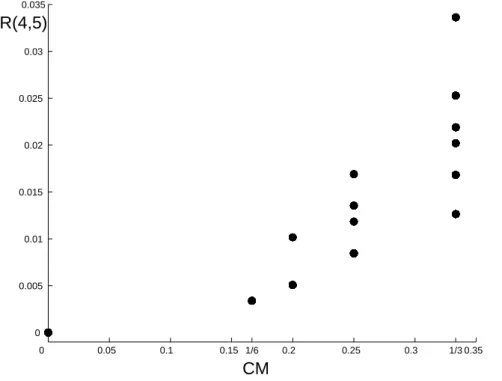
Based on Theorem 4.1 and Table 3, the inconsistency ratio CR(4,5) can be determined. By generating all the possible PRM (9⁶ = 531441 matrices) with CM ≤ 1/3 (1377 matrices) on the ratio scale 1/5, . . . ,1, . . . ,5, Figure 1 shows that the possible values ofCM under1/3 are from the set{0,1/6,1/5,1/4,1/3}and the total number of different pairs (CM, CR(4,5)) is 14. We can state that the threshold CM ≤1/3 corresponds toCR(4,5)≤0.0336 (3.36%). It follows thatKoczkodaj’s inconsistency index for 4×4pairwise comparison matrices with respect to ratio scale1/5, . . . ,1, . . . ,5,is stricter than that ofSaaty’s. It is noted that the10%rule allows much higherCM-inconsistency when using the ratio scale 1/9, . . . ,1, . . . ,9.An example is as follows:

A =







1 1/8 2 6

8 1 7 9

1/2 1/7 1 2 1/6 1/9 1/2 1





,

where CR=CR(4,9) = 9.47% and CM = 0.8125.

(12)

0 0.05 0.1 0.15 1/6 0.2 0.25 0.3 1/3 0.35 0

0.005 0.01 0.015 0.02 0.025 0.03 0.035

CR(4,5)

CM

Figure 1. Koczkodaj’sCM ≤1/3 rule corresponds to CR(4,5)≤3.36%

It is emphasized that the threshold CM ≤1/3is given for 4×4pairwise comparison matrices with respect to the ratio scale1/5, . . . ,1, . . . ,5. A question arises, namely, how to determine the threshold values for higher dimensions. A possible way is to use the

“one grade off” or “two grades off” rules. By Koczkodaj (1997), “An acceptable threshold of inconsistency is0.33because it means that one judgement is not more than two grades of the scale “different” from the remaining two judgements.”

12

(13)

The largest elemen t ( M )

RI(n,M)3456789101112131415 30.1180.1850.2520.3210.3890.4570.5250.5920.6580.7250.7910.8570.922 40.1850.2950.4090.5260.6440.7640.8841.0051.1261.2471.3691.4911.611 50.2250.3610.5040.6510.8020.9551.1091.2641.4211.5781.7351.8942.052 Matrix60.2510.4040.5650.7310.9011.0741.2491.4261.6031.7831.9622.1422.324 size70.2690.4330.6060.7840.9671.1531.3411.5311.7221.9142.1082.3022.496 (n)80.2820.4540.6350.8221.0131.2071.4041.6031.8032.0042.2062.4092.613 90.2920.4700.6570.8501.0471.2481.4511.6561.8622.0692.2782.4872.697 100.3000.4820.6730.8711.0731.2781.4861.6951.9062.1182.3312.5452.759 Table3.AveragevalueoftheinconsistencyindicesofrandomPRMdependingonthelargestelementoftheratioscale

(14)

Let us consider the general form of 3×3 positive reciprocal matrices formulated in (3.1). In the consistent cases, a = b/c, 1/a = c/b, b = ac, 1/b = 1/(ac), c = b/a, 1/c=a/b. In the inconsistent cases, the approximation of an element by the other two elements can be considered by the grade difference

GD(a, b, c) = min n

max{|a−b/c|,|1/a−c/b|}, max{|b−ac|,|1/b−1/(ac)|},max{|c−b/a |,|1/c−a/b |}

o .

Thus, the one grade off rule and the two grades off rule are GD(a, b, c)≤1 and GD(a, b, c)≤2, respectively.

In the case of matrices A of higher orders, the one grade off rule and the two grades off rule (Koczkodaj et al., 1997) are

GD(A) = maxn

GD(a, b, c) for each triad (a, b, c)in Ao

≤ 1 or 2.

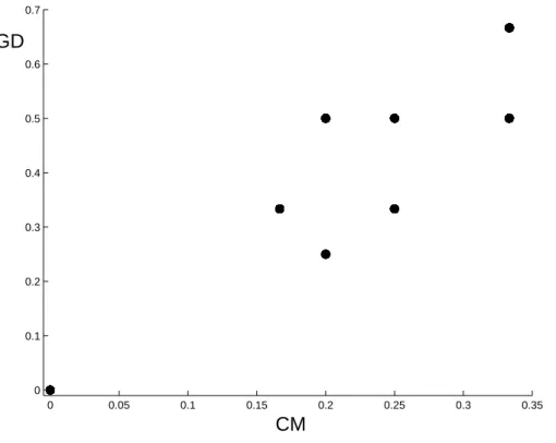
Figure 2 shows that the threshold CM ≤ 1/3 corresponds to GD ≤ 2/3, which is close to the one grade off rule.

0 0.05 0.1 0.15 0.2 0.25 0.3 0.35

0 0.1 0.2 0.3 0.4 0.5 0.6 0.7

CM GD

Figure 2. CM ≤1/3 threshold corresponds to GD≤2/3

14

(15)

5. Inconsistency of random pairwise comparison matrices

Golden and Wang (1990) computed the random inconsistency indices and Forman (1990) the same for incompletePRM.Dodd,Donegan andMcMaster (1993) investigated the frequency distributions of random inconsistency indices and their statistical signif- icance levels. Lane and Verdini (1989) determined the exact distribution of random inconsistency indices for 3× 3 matrices, and random samples of 2500 matrices were produced and analysed for 4×4 to 10×10 and selected higher-order matrices, as well as stricter consistency requirements for 3×3 and 4×4 pairwise comparison matrices were suggested. Standard 2000 generated randomly 1000 PRM, but restricted the CR_n as follows. For n = 3,4 or 5, CR_n < 0.1 was required, for n = 6, CR_n < 0.2, and for n = 7, CR_n < 0.3. The computer was very slow in generating the random, low CR_n, P RM regarding sizes 6 and 7 and the results became more scattered asnincreased. Ad- ditionally, regardingn= 7, there were no results forCR_n <0.1. Due to these conditions, the low CR_n analysis was not run regarding matrices of sizes 8 and 9. A conclusion is that Saaty’s rule is statistically very strict for large PRM.

We have performed a statistical analysis of CR and CM inconsistencies. The aim of our simulation was to analyze the empirical distributions of the maximal eigenvalues λ_max of randomly generated pairwise comparison matrices. The elementsa_ij(i < j)were randomly chosen from the scale

1 9,1

8,1

7, . . . ,1

2,1,2, . . . ,8,9, and a_ji is defined as 1

aij

. In the paper, the assumption of equal probabilities is used.

In order to have equal probabilities (₁₇¹), we used Matlab’s rand function for simulat- ing uniform distribution, the period of which is 2¹⁴⁹². We have computed the average value of λ_max of randomly generated pairwise comparison matrices which is the basis of the mean random consistency index (RI_n). The values of λ_max corresponding to the CRn = 10%, the number of matrices which satisfies the CRn ≤ 10%, GD ≤ 1 and GD ≤2conditions were also computed. (It follows from the definition of CR_n that – if the comparisons are carried out randomly – the expected value of CR_n is 1.) InTable 4, n varies from 3 to 10, the sample size is 10⁷ for all n.

In the case of 3×3 matrices, the sample size 10⁷ is much larger than the number of different matrices 17³ = 4913. Thus, many (or all) of the matrices may have been counted more than once. The ratios of the numbers of matrices holding CR ≤ 10%, GD ≤ 1 and GD ≤ 2 compared to the sample size have been also computed if each matrix counted exactly once, and found to have almost the same results as above.

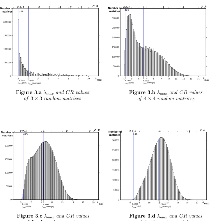
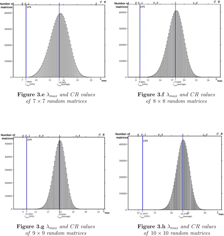
Our simulations are visualized in histograms, too. Figures 3.a –3.h show the empirical distributions ofλ_max on the lower horizontal axis and the corresponding consistency ratio CR_n on the upper horizontal axis. As n increases, the shape of distribution of λ_max gets similar to a normal one in our sample. For n = 3, a notable part of the randomly generated matrices satisfies the CR_n ≤ 10% rule. The number of matrices with CR_n ≤ 10% drastically decreases as n increases (see Table 4). Regarding n = 8,9,10, we have not found a matrix in the sample of ten million with acceptable inconsistency.

Based on the results, it seems that the meaning of 10% for n = 3 is very different from n = 8, which is one of the weaknesses of the inconsistency ratio by Saaty. It is also interesting that consistency and randomness do not exclude each other: 1.7% of 3×3 random matrices (and 0.0014% of 4×4random matrices) are consistent.

(16)

nSample size Average value ofλmaxRInλmax correspondingto CR=10%

Numberof matrices CR≤10%

Numberof matrices GD≤1

Numberof matrices GD≤2 3107 4.04840.52423.10482.08×106 1.42×106 withGD≤1 2.0×106 withGD≤2

1.42×106 allwithCR≤10%2.68×106 2.0×106 withCR≤10% 4107 6.65250.88424.2653.15×105 2.76×104 withGD≤1 1.55×105 withGD≤2

2.76×104 allwithCR≤10%1.7×105 1.55×105 withCR≤10% 5107 9.43471.10875.44352.39×104 61withGD≤1 2371withGD≤2

61 allwithCR≤10%2404 2371withCR≤10% 6107 12.2441.24886.6244770 0withGD≤1 13withGD≤2013 allwithCR≤10% 7107 15.0451.34087.80459 0withGD≤1 0withGD≤200 8107 17.8311.40048.9831000 9107 20.6041.450510.16000 10107 23.3741.48611.3374000 Table4.Averagevalueofλmaxofrandomlygeneratedpairwisecomparisonmatrices,RIn,thenumberofmatriceswithCR≤10%, GD≤1andGD≤2

(17)

6. Inconsistency of asymmetry

A conceptual weakness of some weighting method is related to the issue of asymmetry.

The question: “To what extent does alternative i dominate j?” may be replaced by the question “To what extent is j dominated by i?” The answers to these questions are logically reciprocal. If a technique is applied first to the pairwise comparison matrix A, yielding a solution w, and then to the transposeA^T, yielding a solution w⁰, is wi

w_j = w_j⁰ w⁰_i for every pair (i, j)?

EM does not possess this asymmetry property, since the principal right and left eigenvectors of A are not elementwise reciprocal in the cases of inconsistent pairwise comparison matrices. Consequently, a conceptual limitation of EM is the lack of asymmetry with respect to A and A^T, which means that, for n ≥ 4, there exist, generally, two competing solutions (Johnson et al., 1979). Now, it will be shown that the property of asymmetry is related to the inconsistency.

Definition 6.1 Let A be a pairwise comparison matrix, w and w⁰ the priority vectors of A and A^T, respectively. The invariance under transpose holds if

w_i ≥w_j implies w_i⁰ ≤w_j⁰, ∀(i, j), i, j = 1, . . . , n. (6.1) It follows from the definitions that LSM,χ²M and LLSM defined in Table 1 always fulfil the property of invariance under transpose. SVDM takes this asymmetry, in some sense, into account.

Lemma 6.1 SVDM fulfils the invariance under transpose if and only if uivi+ 1

u_jv_j + 1 ≥ vi

v_j implies uivi+ 1 u_jv_j+ 1 ≤ ui

u_j, ∀(i, j) i, j = 1, . . . , n, (6.2) where u and v are the left and right singular vectors belonging to the largest singular value of A, respectively.

Proof. By the formula in Table 1, the invariance under transpose holds if and only if

ui+ 1

v_i ≥uj + 1

v_j implies vi+ 1

u_i ≤vj + 1

u_j, ∀(i, j) i, j = 1, . . . , n, which is equivalent to

u_iv_i+ 1 u_jv_j + 1 ≥ v_i

v_j implies u_iv_i+ 1 u_jv_j + 1 ≤ u_i

u_j, ∀(i, j) i, j = 1, . . . , n.

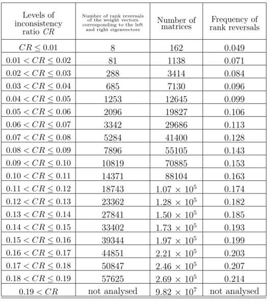
¥ 10⁸ matrices of size 5×5 have been generated randomly in order to detect the rank reversals of the weights computed from the left and right eigenvectors. Based on our hypothesis, the frequency of rank reversals varies as theCR inconsistency ratio changes.

By Table 5 and Figure 4, the frequency of rank reversals increases as the CR increases.

We can conclude that the larger theCR-inconsistency is, the more often theEM violates the property of invariance under transpose. Since no “cut off” point appears inFigure 4, this seems to be another reason for reconsidering the asymmetry property.

(18)

The next example (Dodd et al., 1995) shows that a good inconsistency ratioCR does not exclude the rank reversal between the weights computed from the left and right eigenvectors. Let

A=







1 1 3 9 9

1 1 5 8 5

1/3 1/5 1 9 5 1/9 1/8 1/9 1 1 1/9 1/5 1/5 1 1





 ,

where CR(A) = 0.0820, the weights of the right eigenvector

w^T = (36.5652,38.9564,16.7155,3.4693,4.2936), and the weights of the left eigenvector

w⁰^T = (40.6431,36.4208,15.0669,3.4391,4.4302).

It is interesting that GD(A) = 4.1111. There remain open questions, namely, how to detect and eliminate the inconsistency of asymmetry.

18

(19)

Levels of inconsistency

ratioCR

Number of rank reversals of the weight vectors corresponding to the left

and right eigenvectors

Number of

matrices Frequency of rank reversals

CR≤0.01 8 162 0.049

0.01< CR≤0.02 81 1138 0.071

0.02< CR≤0.03 288 3414 0.084

0.03< CR≤0.04 685 7130 0.096

0.04< CR≤0.05 1253 12645 0.099

0.05< CR≤0.06 2096 19827 0.106

0.06< CR≤0.07 3342 29686 0.113

0.07< CR≤0.08 5284 41400 0.128

0.08< CR≤0.09 7896 55105 0.143

0.09< CR≤0.10 10819 70885 0.153

0.10< CR≤0.11 14371 88104 0.163

0.11< CR≤0.12 18743 1.07 × 10⁵ 0.174

0.12< CR≤0.13 23362 1.28 × 10⁵ 0.182

0.13< CR≤0.14 27841 1.50 × 10⁵ 0.185

0.14< CR≤0.15 33402 1.73 × 10⁵ 0.193

0.15< CR≤0.16 39344 1.97 × 10⁵ 0.199

0.16< CR≤0.17 44851 2.21 × 10⁵ 0.203

0.17< CR≤0.18 50847 2.46 × 10⁵ 0.207

0.18< CR≤0.19 57625 2.69 × 10⁵ 0.214

0.19< CR not analysed 9.82 × 10⁷ not analysed

Table 5. Frequency of rank reversals of the weight vectors corresponding to the left and right eigenvectors with respect to different levels of inconsistency ratio CR

Figure 4. Frequency of rank reversals of the weight vectors corresponding to the left and right eigenvectors with respect to different levels of inconsistency ratioCR

(20)

7. Concluding remarks

In the paper, some theoretical and numerical properties of Saaty’s and Koczkodaj’s inconsistencies of PRM are investigated. Based on the results, it seems that the deter- mination of the inconsistency ofPRM has some drawbacks, thus the improvement of the notion of inconsistency should be necessary.

Related to Saaty’s inconsistency ratio, some basic questions are as follows:

What is the relation between an empirical matrix from human judgements and a randomly generated one? Is an index obtained from several hundreds of randomly generated matrices the right reference point for determining the level of inconsistency of pairwise comparison matrix built up from human decisions, for a real decision problem? How to take the size of matrices into account in a more precise form?

Related to Koczkodaj’s consistency index, a major question seems to be the elabora- tion of the thresholds in higher dimensions or to replace the index by a refined grade off rule.

The existence of the inconsistency of asymmetry shows the complexity of the problem.

By the example inSection 6,Saaty’s consistency ofPRM is insufficient to exclude asym- metric inconsistency, therefore, this latter should be considered as a separate issue. Thus, it seems that only one inconsistency index is insufficient for describing the inconsistency.

Acknowledgement

The authors thank the Referees for the remarks and advice. The distinction ofSaaty’s and Koczkodaj’s inconsistencies, given by one of the Referees, is emphasized.

20

(21)

References

Aguarón, J. and Moreno-Jiménez, J.M., The geometric consistency index: Approxi- mated thresholds,European Journal of Operational Research 147 (2003) 137-145.

Borda, J.C. de, Mémoire sur les électiones au scrutin, Histoire de l’Académie Royale des Sciences,Paris, 1781.

Chu, A.T.W., Kalaba, R.E. and Spingarn, K., A comparison of two methods for determining the weight belonging to fuzzy sets, Journal of Optimization Theory and Applications 4 (1979) 531-538.

Condorcet, M., Essai sur l’application de l’analyse à la probabilité des décisions rendues á la pluralité des voix, Paris, 1785.

Crawford, G. and Williams, C., A note on the analysis of subjective judgment matrices, Journal of Mathematical Psychology 29 (1985) 387-405.

Dodd, F.J., Donegan, H.A. and McMaster, T.B.M., A statistical approach to consistency in AHP, Mathematical and Computer Modelling 18 (1993) 19-22.

Dodd, F.J., Donegan, H.A. and McMaster, T.B.M., Inverse inconsistency in analytic hierarchy process,European Journal of Operational Research 80 (1995) 86-93.

Duszak, Z. and Koczkodaj, W.W., Generalization of a new definition of consistency for pairwise comparisons, Information Processing Letters 52 (1994) 273-276.

Forman, E.H., Random indices for incomplete pairwise comparison matrices, European Journal of Operational Research 48 (1990) 153-155.

Gass, S.I. and Rapcsák, T., Singular value decomposition in AHP,European Journal of Operational Research 154 (3) (2004) 573-584.

Gass, S.I. and Standard, S.M., Characteristics of positive reciprocal matrices in the analytic hierarchy process, Journal of Operational Research Society 53 (2002) 1385-1389.

Golden, B.L. and Wang, Q., An alternative measure of consistency, in: Analytic Hierarchy Process: Applications and Studies, B.L. Golden, E.A. Wasil and P.T. Hacker (eds.), Springer-Verlag (1990) 68-81.

Jensen, R.E., Comparison of eigenvector, least squares, Chi square and logarithmic least squares methods of scaling a reciprocal matrix, Trinity University, Working Paper 127 (1983). (http://www.trinity.edu/rjensen/127wp/127wp.htm)

Johnson, C.R., Beine, W.B. and Wang, T.J., Right-left asymmetry in an eigenvector ranking procedure, Journal of Mathematical Psychology 19 (1979) 61-64.

Koczkodaj, W.W., A new definition of consistency of pairwise comparisons, Mathematical and Computer Modelling 8 (1993) 79-84.

Koczkodaj, W.W., Herman, M.W. and Orlowski, M., Using consistency-driven pairwise comparisons in knowledge-based systems, in: Proceedings of the sixth international conference on Information and knowledge management, ACM Press (1997) 91-96.

(22)

Lane, E.F. and Verdini, W.A., A consistency test for AHP decision makers, Decision Sciences 20 (1989) 575-590.

Monsuur, H., An intrinsic consistency threshold for reciprocal matrices, European Journal of Operational Research 96 (1996) 387-391.

Murphy, C.K., Limits on the analytic hierarchy process from its consistency index, European Journal of Operational Research 65 (1993) 138-139.

Peláez, J.I. and Lamata, M.T., A new measure of consistency for positive reciprocal matrices, Computers and Mathematics with Applications 46 (2003) 1839-1845.

Saaty, T.L., The analytic hierarchy process, McGraw-Hill, New York, 1980 and 1990.

Saaty, T.L., Fundamentals of Decision Making,RSW Publications, 1994.

Standard, S.M., Analysis of positive reciprocal matrices, Master’s Thesis, Graduate School of the University of Maryland, 2000.

Stein, W.E. and Mizzi, P.J., The harmonic consistency index for the analytic hierarchy process, European Journal of Operational Research 177 (2007) 488-497.

Thorndike, E.L., A constant error in psychological ratings, Journal of Applied Psychology 4 (1920) 25-29.

Thurstone, L.L., The method of paired comparisons for social values, Journal of Abnormal and Social Psychology 21 (1927) 384-400.

Tummala, V.M.R. and Ling, H., A note on the computation of the mean random consistency index of the analytic hierarchy process (AHP), Theory and Decision 44 (1998) 221-230.

Vargas, L.G., Reciprocal matrices with random coefficients, Mathematical Modelling 3 (1982) 69-81.

22

(23)

List of Figures 3

3 4 5 6 7 8 9 10

0 500000 1000000 1500000 2000000

λ_max Number of

matrices

0 1 2 3 4 5 6 C R

3.1048 4.0484 λ_max(10%)λ_max(average)

0.1 10%

4 5 6 7 8 9 10 11 12 13 14

0 50000 100000 150000 200000 250000 300000

matrices

0 1 2 3 C R

4.2652 6.6525

λ_max(10%) λ_max(average) 0.1

10%

Figure 3.a λmax and CR values of 3×3random matrices

Figure 3.b λmax and CR values of 4×4 random matrices

5 7 9 11 13 15 17 19

0 50000 100000 150000 200000

matrices

0 1 2 3 C R

5.4435 9.4347

10%

6 8 10 12 14 16 18 20

0 50000 100000 150000 200000 250000 300000

matrices

0 1 2 C R

6.6244 12.2442

10%

Figure 3.cλmax and CR values of 5×5 random matrices

Figure 3.d λmax and CRvalues of 6×6 random matrices

(24)

7 10 13 16 19 22 0

100000 200000 300000 400000

matrices

0 1 2 C R

7.8045 15.0452

λ_max(10%) λ_max(average)

0.1 10%

8 11 14 17 20 23 26

0 100000 200000 300000 400000

λmax Number of

matrices

0 0.5 1 1.5 C R

8.9831 17.8309

0.1 10%

Figure 3.e λ_max and CR values of 7×7 random matrices

Figure 3.f λ_max and CRvalues of 8×8 random matrices

9 13 17 21 25 29 33

0 100000 200000 300000 400000 500000

matrices

0 0.5 1 1.5 C R

10.1604 20.6044

0.1 10%

10 15 20 25 30

0 100000 200000 300000 400000

matrices

0 0.5 1 1.5 C R

11.3374 23.3743

0.1 10%

Figure 3.g λ_max and CR values of 9×9 random matrices

Figure 3.h λ_max and CR values of 10×10 random matrices

24