Efficiency analysis of double perturbed pairwise comparison matrices
Kristóf Ábele-Nagy
1,2∗Sándor Bozóki
1,2†Örs Rebák
‡Abstract
Efficiency is a core concept of multi-objective optimization problems and multi-attribute decision making. In the case of pairwise comparison matrices a weight vector is called efficient if the approximations of the elements of the pairwise comparison matrix made by the ratios of the weights cannot be improved in any position without making it worse in some other position. A pairwise comparison matrix is called double perturbed if it can be made consistent by altering two elements and their reciprocals. The most frequently used weighting method, the eigenvector method is analyzed in the paper, and it is shown that it produces an efficient weight vector for double perturbed pairwise comparison matrices.
Keywords: pairwise comparison matrix, efficiency, Pareto optimality, eigen- vector
1 Introduction
Ranking alternatives, or picking the best alternative is a commonly investigated prob- lem. The case of a single cardinal objective function to be maximized or minimized is long studied by various operations research disciplines. This is however often not feasible. Alternatives can be ranked by assigning a cardinal utility to them, or by set- ting up ordinal preference relations among them. In the case of a single criterion and a single decision maker, modelling the preferences is often possible through standard methods. If there are multiple, often contradicting criteria, this becomes significantly harder. A dominant alternative, which is the best with respect to all criteria, very rarely exists. Thus, when a decision making method is used to aid the decision of a decision maker, some form of compromise is needed. Modelling the preferences of the decision maker by ranking or weighting the criteria can accomplish such a compro- mise. It allows the “best” alternative to be chosen (or the possible alternatives to be
∗E-mail: kristof.abele-nagy@uni-corvinus.hu
†E-mail: bozoki.sandor@sztaki.mta.hu
‡E-mail: rebakors@gmail.com
1Laboratory on Engineering and Management Intelligence, Research Group of Operations Research and Decision Systems, Institute for Computer Science and Control, Hungarian Academy of Sciences;
Mail: 1518 Budapest, P.O. Box 63, Hungary.
2Department of Operations Research and Actuarial Sciences, Corvinus University of Budapest, Hungary
arXiv:1602.07137v2 [math.OC] 11 Sep 2018
Manuscript of / please cite as
Ábele-Nagy, K., Bozóki, S., Rebák, Ö. [2018]:
Efficiency analysis of double perturbed pairwise comparison matrices, Journal of the Operational Research Society
69(5), pp.707-713.
http://dx.doi.org/10.1080/01605682.2017.1409408
ranked) with respect to the subjective preferences of the decision maker. Examples of multi-criteria decision problems range from “Which house to buy?” or “What should the company invest in?” to public tenders.
When weighting criteria, giving the weights directly is almost never feasible. In- stead, a common method is to apply pairwise comparisons. Answers to the questions
“How many times is Criterion A more important than Criterion B?” and so on (which are explicit cardinal ratios) can be arranged in a matrix, called a pairwise compari- son matrix (PCM). Formally, a PCM is a square matrix A = [aij]i,j=1,...,n with the properties aij >0 and aij = 1/aji (which implies aii = 1). If the cardinal transitivity property aikakj = aij for all i, j, k = 1, . . . , n also holds for a PCM, it is called con- sistent, otherwise it is called inconsistent [21]. Let PCMn denote the set of PCMs of size n×n. The next step is to extract the weights of criteria from the PCM. Several methods exist for this task [3, 10, 13, 18]. The eigenvector method (EM) is one of the classical [21], important and most often studied weighting methods related to pairwise comparison matrices, its further analysis is actual and relevant both in decision theory and operations research. We focus on EM in this paper. The eigenvector method gives the weight vectorwEM = (w1, . . . , wn)T as the right Perron eigenvector ofA ∈ PCMn, thusAwEM =λmaxwEM holds, whereλmaxis the principal eigenvalue ofA. λmax ≥n, and λmax =n if and only if A is consistent [21]. A consistent PCM can be written as
A=
1 x1 x2 . . . xn−1
1/x1 1 x2/x1 . . . xn−1/x1 1/x2 x1/x2 1 . . . xn−1/x2
... ... ... . .. ... 1/xn−1 x1/xn−1 x2/xn−1 . . . 1
∈ PCMn,
where x1, . . . , xn−1 >0.
The elements of a PCM approximate the ratios of the weights, therefore the ratios of the elements of the weight vector should be as close as possible to the corresponding matrix elements. If a weight vector cannot be trivially improved in this regard (there is no other weight vector which is at least as good approximation, and strictly better in at least one position), it is called Pareto optimal or efficient. It has been proved that the eigenvector method does not always produce an efficient solution [4, Section 3]. However, in some special cases the eigenvector method always gives an efficient weight vector. If the PCM is simple perturbed, i.e., it differs from a consistent PCM in only one element and its reciprocal, the principal right eigenvector is efficient [1].
In the paper this will be extended to double perturbed PCMs, which only differ from a consistent PCM in two elements and their reciprocals.
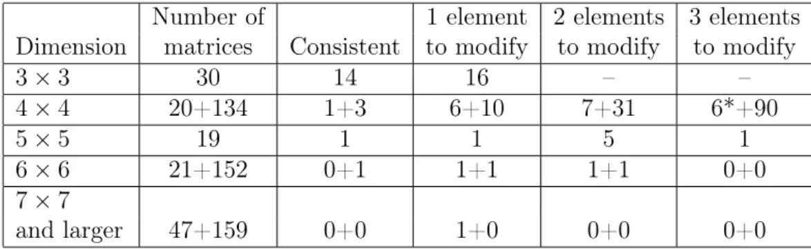
These special types of PCMs are not just theoretically important, but also occur in real decision problems. Poesz [20] gathered a handful of empirical PCMs that were analyzed in [8]. Although double perturbed PCMs are rare among large PCMs, they appear more frequently among smaller matrices, in other words, when the number of criteria is small. This is especially true if one considers simple perturbed and consistent PCMs as special cases of double perturbed PCMs (see [8, Table 1] – note there is a misprint in the cited Table, the number in the “3 elements to modify” column in the 4×4 row should be 6 instead of 0). We also conducted an analysis of the prevalence of double perturbed PCMs among the empirical matrices analyzed in [6]. Below is a
Number of 1 element 2 elements 3 elements Dimension matrices Consistent to modify to modify to modify
3×3 30 14 16 – –
4×4 20+134 1+3 6+10 7+31 6*+90
5×5 19 1 1 5 1
6×6 21+152 0+1 1+1 1+1 0+0
7×7
and larger 47+159 0+0 1+0 0+0 0+0
Table 1: The number of element modifications needed to get a consistent PCM.
*There was a misprint in [8, Table 1], this number was 0. The correct value is 6.
in [6] had sizes 4×4, 6×6 and 8×8. The numbers after the + sign are from [6], all others are from [8]. As it can be seen from Table 1, double (and less) perturbed PCMs are rare among large matrices, but they appear among smaller ones.
In Section 2 we will introduce the key definitions and tools used in the paper, together with an example. In Section 3 the main result of the paper is presented:
through obtaining explicit formulas for the principal right eigenvector and a series of lemmas, the efficiency of the principal right eigenvector is shown for the case of double perturbed PCMs. The proofs of the lemmas, are given in detail in the Appendix. In Section 4 conclusions follow.
2 Efficiency and perturbed pairwise comparison ma- trices
The general form of a multi-objective optimization problem ([14, Chapter 2][23, Chap- ter 6]) is
min{f1(y), f2(y), . . . , fm(y), . . . , fM(y)}
subject toy∈S
whereM ≥2denotes the number of objective functions,fm :Rn→Rfor all1≤m≤ M. Variables arey= (y1, y2, . . . , yn) and the feasible set is denoted by S ⊆Rn.
Efficiency or Pareto optimality is a basic concept of multi-objective optimization and multi-attribute decision making, too. A vector y ∈ S is called efficient, if there does not exist another vector y0 ∈ S such that fm(y0) ≤ fm(y) for all 1 ≤ m ≤ M, and fk(y0)< fk(y) for at least one index k.
Let A = [aij]i,j=1,...,n ∈ PCMn and w = (w1, w2, . . . , wn)T be a positive weight vector (S =Rn++,the positive orthant of then-dimensional Euclidean space), wheren is the number of criteria. Let us specify the objective functions byfij(w) :=
aij− wwi
j
for all i6=j. We have M =n2 −n objective functions.
Definition 1. A positive weight vectorwis calledefficient if no other positive weight vector w0 = (w01, w20, . . . , wn0)T exists such that
aij − wi0 wj0
≤
aij − wi
wj
for all 1≤i, j ≤n, (1)
ak`− wk0 w`0
<
ak`− wk w`
for some 1≤k, `≤n. (2) A weight vector wis called inefficient if it is not efficient.
It follows from the definition that an arbitrary renormalization does not influence (in)efficiency.
Remark 1. Weight vector w is efficient if and only if cw is efficient for any c >0.
For a consistent PCM aij = wEMi /wEMj for all i, j = 1, . . . , n [21], which implies the following remark:
Remark 2. The principal right eigenvectorwEM is efficient for every consistent PCM.
For inconsistent PCMs however, the principal right eigenvector can be inefficient, found by Blanquero, Carrizosa and Conde [4, Section 3]. This result was also rein- forced by Bajwa, Choo and Wedley [3], by Conde and Pérez [11] and by Fedrizzi [17].
Blanquero, Carrizosa and Conde [4] developed LP models to test whether a weight vector is efficient. Bozóki and Fülöp [7] further developed the models and provided algorithms to improve an inefficient weight vector. Anholcer and Fülöp [2] devised a new algorithm to derive an efficient solution from an inconsistent PCM.
Furthermore, Bozóki [5] showed that the principal right eigenvector of a whole class of matrices, namely the parametric PCM
A(p, q) =
1 p p p . . . p p
1/p 1 q 1 . . . 1 1/q 1/p 1/q 1 q . . . 1 1
... ... ... . .. ... ... ... ... ... . .. ... ...
1/p 1 1 1 . . . 1 q
1/p q 1 1 . . . 1/q 1
∈ PCMn,
where n≥4, p >0 and 16=q >0, is inefficient.
Several necessary and sufficient conditions were examined by Blanquero, Carrizosa and Conde [4], one of which is of crucial importance here. It uses a directed graph representation as follows:
Definition 2. LetA= [aij]i,j=1,...,n ∈ PCMn andw= (w1, w2, . . . , wn)T be a positive weight vector. A directed graphG= (V,−→
E)A,wis defined as follows: V ={1,2, . . . , n}
and −→
E =
arc(i→j)
wi
wj ≥aij, i6=j
.
It follows from Definition 2 that if wi/wj = aij, then there is a bidirected arc between nodes i and j. The result of Blanquero, Carrizosa and Conde using this
Theorem 1 ([4, Corollary 10]). Let A ∈ PCMn. A weight vector w is efficient if and only if G= (V,−→
E)A,w is a strongly connected digraph, that is, there exist directed paths from i to j and from j to i for all pairs of nodes i, j.
The following numerical example provides an illustration for Theorem 1.
Example 1. Let A∈ PCM4 be as follows:
A=
1 1 4 7
1 1 7 4
1/4 1/7 1 3
1/7 1/4 1/3 1
.
The principal right eigenvectorwEM and the consistent approximation ofAgenerated bywEM are as follows:
wEM =
0.39940672 0.43144159 0.10721105 0.06194064
,
wEMi wEMj
=
1 0.9257 3.7254 6.4482 1.0802 1 4.0242 6.9654 0.2684 0.2485 1 1.7309 0.1551 0.1436 0.5777 1
.
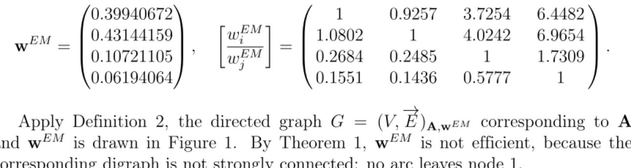
Apply Definition 2, the directed graph G = (V,−→
E)A,wEM corresponding to A and wEM is drawn in Figure 1. By Theorem 1, wEM is not efficient, because the corresponding digraph is not strongly connected: no arc leaves node 1.
4 1
2
3
Figure 1: The principal right eigenvector in Example 1 is inefficient, because the corresponding digraph is not strongly connected: no arc leaves node 1
It can be seen in a more constructive way why the principal right eigenvector wEM is inefficient. Increase the first coordinate until 0.428844188, and keep the other coordinates unchanged:
w0 =
0.428844188 0.431441588 0.107211052 0.061940644
,
w0i w0j
=
1 0.9940 4 6.9235
1.0061 1 4.0242 6.9654
1/4 0.2485 1 1.7309
0.1444 0.1436 0.5777 1
.
The approximation in the entries marked by bold became strictly better ((2) holds in Definition 1), while for all other entries the approximation remained the same ((1)
holds with equality in Definition 1).
As it can be seen from Example 1 above, Theorem 1 is a powerful an applicable characterization of efficiency.
Open problem 1. What is the necessary and sufficient condition of the principal right eigenvector’s efficiency?
In the rest of the paper, special types of PCMs are considered.
A simple perturbed PCM differs from a consistent PCM in only one element and its reciprocal, or in other words it can be made consistent by altering only one element (and its reciprocal). Thus, without loss of generality, a simple perturbed PCM can be written as
Aδ =
1 δx1 x2 . . . xn−1
1/(δx1) 1 x2/x1 . . . xn−1/x1
1/x2 x1/x2 1 . . . xn−1/x2 ... ... ... . .. ... 1/xn−1 x1/xn−1 x2/xn−1 . . . 1
∈ PCMn,
where x1, . . . , xn−1 >0 and 0< δ 6= 1.
Theorem 2 ([1, Theorem 3.1]). The principal right eigenvector of a simple perturbed pairwise comparison matrix is efficient.
Similarly, a double perturbed PCM differs from a consistent PCM in two elements and their reciprocals, or in other words it can be made consistent by altering two elements (and their reciprocals). We have to differentiate between three cases of double perturbed PCMs. Without loss of generality, every double perturbed PCM is equivalent to one of them. Also, we can suppose without the loss of generality, that from now onn≥4, because a PCM withn= 3is either simple perturbed or consistent.
In Case 1, the perturbed elements are in the same row, and they are multiplied by 0< δ 6= 1 and 0< γ 6= 1 respectively. In Case 2, they are in different rows, but this case needs to be further divided into two subcases (2A and 2B) due to algebraic issues.
In Case 2A matrix size is 4×4, while in Case 2B matrix size is at least 5×5. Thus, these matrices take the following form:
Case 1:
Pγ,δ =
1 δx1 γx2 x3 . . . xn−1
1/(δx1) 1 x2/x1 x3/x1 . . . xn−1/x1 1/(γx2) x1/x2 1 x3/x2 . . . xn−1/x2 1/x3 x1/x3 x2/x3 1 . . . xn−1/x3
... ... ... ... . .. ... 1/xn−1 x1/xn−1 x2/xn−1 x3/xn−1 . . . 1
, (3)
Case 2A:
Qγ,δ =
1 δx1 x2 x3
1/(δx1) 1 x2/x1 x3/x1 1/x2 x1/x2 1 γx3/x2
, (4)
Case 2B:
Rγ,δ =
1 δx1 x2 x3 x4 . . . xn−1
1/(δx1) 1 x2/x1 x3/x1 x4/x1 . . . xn−1/x1 1/x2 x1/x2 1 γx3/x2 x4/x2 . . . xn−1/x2
1/x3 x1/x3 x2/(γx3) 1 x4/x3 . . . xn−1/x3 1/x4 x1/x4 x2/x4 x3/x4 1 . . . xn−1/x4
... ... ... ... ... . .. ...
1/xn−1 x1/xn−1 x2/xn−1 x3/xn−1 x4/xn−1 . . . 1
. (5)
Once again, x1, . . . , xn−1 >0 and 0< δ, γ 6= 1.
Remark 3. If either δ= 1 or γ = 1 then the PCM is simple perturbed. If δ =γ = 1 then the PCM is consistent.
Remark 4. If n = 4 and δ = γ, then the PCM Pδ,δ in Case 1 is simple perturbed (multiply the single element x3 in position (1,4) by δ to have a consistent PCM).
Bozóki, Fülöp and Poesz examined PCMs that can be made consistent by modify- ing at most 3 elements [8]. Each of the three cases above corresponds to a graph: Case 1 corresponds to [8, Fig. 6(b)] while Case 2 corresponds to [8, Fig. 6(a)]. Cook and Kress [12] and Brunelli and Fedrizzi [9] also examined the similar idea of comparing two PCMs that differ in only one element.
3 Main result: the principal right eigenvector of a double perturbed PCM is efficient
The main result of the paper is the extension of Theorem 2 for double perturbed PCMs.
Theorem 3. The principal right eigenvector of a double perturbed PCM is efficient.
Proof. For the purpose of easy readability, only an outline of the proof is presented here. The detailed proof can be found in the Appendix.
A method to acquire the explicit form of the principal right eigenvector of a PCM when the perturbed elements are in the same row or column has been developed by Farkas, Rózsa and Stubnya [16]. Farkas [15] writes the explicit formula for the simple perturbed case. Our first goal is to extend the method for the double perturbed case.
Similar to [15], the characteristic polynomial is needed first. Proposition 1 covers Case 1 and Proposition 2 covers Cases 2A and 2B.
Using the formulas for the characteristic polynomial, explicit formulas can be de- rived for the principal right eigenvector. Proposition 3 presents these formulas. For each Case the formulas can be written in several different forms.
Utilizing the different explicit formulas for the principal right eigenvector a series of inequalities can be proved. These inequalities are presented in 28 lemmas (Lemmas 1a–3h). The different forms of the formula for the principal right eigenvector make it possible to use the form most suited to each proof. Obtaining these inequalities makes it possible to prove the efficiency of the principal right eigenvector of a double perturbed PCM.
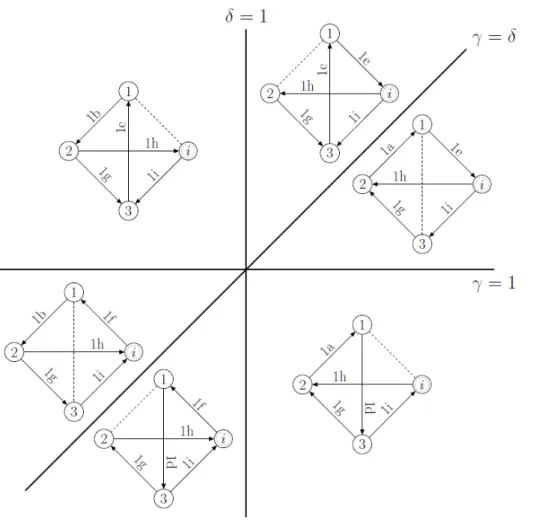
As per Theorem 1, the strong connectedness of the digraph in Definition 2 needs to be shown. All possible digraphs are shown in Figures 2–4. The direction of each arc (where applicable) is determined by the corresponding Lemma using Definition 2, which is labeled on the arc itself. In the cases where there is a node named i, this represents the complete subgraph of the rest of the nodes (consisting of n−3in Case 1 and n−4 nodes in Case 2B). In these subgraphs there are bidirected arcs between any two nodes, due to Lemmas 1j and 3h. This is a strongly connected subgraph, and for any fixed j ≤ 3 the direction of the arc between nodes i and j is the same for every i ≥ 4 in Case 1 (see Lemmas 1e, 1f, 1h, 1i). Similarly, for any fixed j ≤ 4 the direction of the arc between nodes iand j is the same for every i≥5 in Case 2B (see Lemmas 3c, 3d, 3e). Hence, it can be contracted into a single node when analyzing strong connectedness. Figures 2, 3, 4 correspond to Cases 1, 2A, 2B respectively.
For the strong connectedness of each digraph, it is sufficient to find a directed cycle.
Unchecked arcs are denoted by dashed lines in Figures 2–4. The directed cycles are presented in Corollary 1, 2 and 3 for Cases 1, 2A and 2B respectively.
The presence of a directed cycle implies strong connectedness for all of the digraphs, which implies efficiency in all cases by Theorem 1.
Figure 2: The digraph of the principal right eigenvector in Case 1 is strongly connected, independently of the orientation of dashed arcs that have not been analyzed
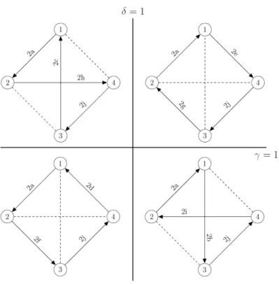
Figure 3: The digraph of the principal right eigenvector in Case 2A is strongly connected, independently of the orientation of dashed arcs that have not been analyzed
Figure 4: The digraph of the principal right eigenvector in Case 2B is strongly connected, independently of the orientation of dashed arcs that have not been analyzed
4 Conclusions
In the paper we used linear algebraic methods to derive explicit formulas for the prin- cipal eigenvector of double perturbed PCMs. We also used a necessary and sufficient condition for efficiency which uses a directed graph representation (the weight vector is efficient if and only if this graph is strongly connected) developed by Blanquero, Carrizosa and Conde [4]. Double perturbed PCMs had to be divided into three cases in order to get explicit formulas for every case. In all three cases the digraph has been studied arc by arc, however not all arcs had to be studied in order to determine strong connectedness. Utilizing all these tools, we have shown in the paper, that the often used eigenvector method produces an efficient weight vector in the case of double perturbed PCMs. This is an extension of our earlier result for simple perturbed PCMs [1].
A direct extension to the triple (or more) perturbed case is not possible, since all PCMs of at least 4×4 size which are not (at most) double perturbed are triple perturbed, and there are examples, e.g. Example 1, of inefficiency of size4×4. Thus, while in some cases (e.g. when all perturbed elements are in different rows/columns) it may be possible to show efficiency, for all triple perturbed PCMs this is impossible.
Furthermore, a triple perturbed PCM can be equivalent to five separate basic cases (see [8, Fig. 7]), which may need to be further divided into more subcases, making the efficiency analysis of triple perturbed PCMs difficult. A full characterization of the efficiency of the principal right eigenvector is still an open question, and a possible subject of future research.
Acknowledgements
The authors are grateful to the anonymous reviewers for their constructive remarks.
András Farkas (Óbuda University, Budapest) and János Fülöp (Institute for Computer Science and Control, Hungarian Academy of Sciences (MTA SZTAKI) and Óbuda University, Budapest) are greatly acknowledged for their valuable comments. Research was supported in part by the Hungarian Scientific Research Fund (OTKA) grant K 111797. S. Bozóki acknowledges the support of the János Bolyai Research Fellowship no. BO/00154/16/3.
References
[1] K. Ábele-Nagy and S. Bozóki. Efficiency analysis of simple perturbed pairwise comparison matrices. Fundamenta Informaticae, 144(3-4):279–289, 2016.
[2] M. Anholcer and J. Fülöp. Deriving priorities from inconsistent PCM using the network algorithms. Under review, http://arxiv.org/pdf/1510.04315, 2017.
[3] G. Bajwa, E. U. Choo, and W. C. Wedley. Effectiveness analysis of deriving pri- ority vectors from reciprocal pairwise comparison matrices. Asia-Pacific Journal of Operational Research, 25(3):279–299, 2008.
[4] R. Blanquero, E. Carrizosa, and E. Conde. Inferring efficient weights from pairwise comparison matrices. Mathematical Methods of Operations Research, 64(2):271–284, 2006.
[5] S. Bozóki. Inefficient weights from pairwise comparison matrices with arbitrarily small inconsistency. Optimization, 63(12):1893–1901, 2014.
[6] S. Bozóki, L. Dezső, A. Poesz, and J. Temesi. Analysis of pairwise comparison matrices: an empirical research. Annals of Operations Research, 211(1):511–528, feb 2013.
[7] S. Bozóki and J. Fülöp. Efficient weight vectors from pairwise comparison matri- ces. European Journal of Operational Research, 264(2):419–427, 2018.
[8] S. Bozóki, J. Fülöp, and A. Poesz. On pairwise comparison matrices that can be made consistent by the modification of a few elements. Central European Journal of Operations Research, 19(2):157–175, 2011.
[9] M. Brunelli and M. Fedrizzi. Axiomatic properties of inconsistency indices for pairwise comparisons. Journal of the Operational Research Society, 66(1):1–15, 2014.
[10] E. Choo and W. Wedley. A common framework for deriving preference values from pairwise comparison matrices. Computers & Operations Research, 31(6):893–908, 2004.
[11] E. Conde and M. d. l. P. R. Pérez. A linear optimization problem to derive relative weights using an interval judgement matrix. European Journal of Operational Research, 201(2):537–544, 2010.
[12] W. Cook and M. Kress. Deriving weights from pairwise comparison ratio matrices:
An axiomatic approach. European Journal of Operational Research, 37(3):355–
362, 1988.
[13] T. K. Dijkstra. On the extraction of weights from pairwise comparison matrices.
Central European Journal of Operations Research, 21(1):103–123, 2013.
[14] M. Ehrgott. Multicriteria Optimization. Volume 491 of Lecture Notes in Eco- nomics and Mathematical Systems. Springer Verlag, Berlin, 2000.
[15] A. Farkas. The analysis of the principal eigenvector of pairwise comparison ma- trices. Acta Polytechnica Hungarica, 4(2):99–115, 2007.
[16] A. Farkas, P. Rózsa, and E. Stubnya. Transitive matrices and their applications.
Linear Algebra and its Applications, 302–303:423–433, 1999.
[17] M. Fedrizzi. Obtaining non-dominated weights from preference relations through norm-induced distances. XXXVII Meeting of the Italian Association for Math- ematics Applied to Economic and Social Sciences (AMASES), September 5–7, 2013, Stresa, Italy, 2013.
[18] B. Golany and M. Kress. A multicriteria evaluation of methods for obtaining weights from ratio-scale matrices. European Journal of Operational Research, 69(2):210–220, 1993.
[19] D. A. Harville. Matrix Algebra From a Statistician’s Perspective. Springer, 2008.
[20] A. Poesz. Empirical pairwise comparison matrices (EPCM) – an on-line collection from real decisions, version EPCM-October-2009.
http://www.sztaki.hu/%7ebozoki/epcm, 2009.
[21] T. L. Saaty. A scaling method for priorities in hierarchical structures. Journal of Mathematical Psychology, 15(3):234–281, 1977.
[22] J. Sherman and W. J. Morrison. Adjustment of an inverse matrix corresponding to a change in one element of a given matrix. Annals of Mathematical Statistics, 21(1):124–127, 1950.
[23] R. E. Steuer. Multiple Criteria Optimization: Theory, Computation, and Appli- cation. Wiley Series in Probability and Mathematical Statistics. Wiley, 1986.
Appendix
Let D= diag(1,1/x1, . . . ,1/xn−1), and let e= (1, . . . ,1)T. For A∈ PCMn,
eeT −UiVTi =D−1AD (6) holds for i= 1,2. For i= 1, A has form (3) (Case 1) and
U1 =
0 1
1−1/δ 0 1−1/γ 0
0 0
... ...
0 0
∈Rn×2, V1 =
1 0
0 1−δ 0 1−γ
0 0
... ...
0 0
∈Rn×2. (7)
For i= 2, A has form (4) or (5) (Case 2) and
U2 =
0 1 0 0
1−1/δ 0 0 0
0 0 0 1
0 0 1−1/γ 0
0 0 0 0
... ... ... ...
0 0 0 0
∈Rn×4,V2 =
1 0 0 0
0 1−δ 0 0
0 0 1 0
0 0 0 1−γ
0 0 0 0
... ... ... ...
0 0 0 0
∈Rn×4. (8)
Lemma 1 (Matrix determinant lemma, [19]). If A ∈Rn×n is invertible, and U,V ∈ Rn×m, then
det(A+UVT) = det(Im+VTA−1U) det(A), where Im denotes the identity matrix of size m×m.
Lemma 2 (Sherman–Morrison formula, [22]). Let A ∈ Rn×n, u,v ∈ Rn. If A is invertible and 1 +vTA−1u 6= 0, then A+uvT−1
exists, and A+uvT−1
=A−1− 1
1 +vTA−1uA−1uvTA−1.
Let A ∈ PCMn be a double perturbed PCM and Ui,Vi be as in (6). Let the matrix KA(λ)∈Rn×n be defined as follows:
KA(λ) = λI+UiVTi −eeT =λI−D−1AD,
where I denotes In, e = (1, . . . ,1)T ∈ Rn, i = 1 in Case 1, i = 2 in Case 2, and the second equation follows from (6).
Lemma 3. The characteristic polynomial of the double perturbed PCM A ∈ PCMn is
pA(λ) = (−1)ndet(KA(λ)).
Proof. As before,i= 1 in Case 1 and i= 2 in Case 2.
pA(λ) = det(A−λI)
= (−1)ndet(λI−A)
= (−1)ndet λI+D UiViT −eeT D−1
= (−1)ndet D λI+UiViT −eeT D−1
= (−1)ndet(D) det λI+UiVTi −eeT
det D−1
= (−1)ndet(KA(λ)).
Lemma 4. det(λI−eeT) =λn−nλn−1.
Proof. If λ= 0, then both sides of the equation are 0. Ifλ6= 0, apply Lemma 1 with m= 1, A=λI, U=−e, V=e:
det(λI−eeT) = (1−eT(λI)−1e) det(λI) = λn−nλn−1.
Lemma 5. If λ6= 0 and λ6=n, then λI−eeT−1
exists, and λI−eeT−1
= 1
λ(λ−n)eeT + 1 λI.
Proof. Apply the Sherman–Morrison formula (Lemma 2) with A = λI, u = −e, v=e.
Lemma 6. Let U,V ∈Rn×m be arbitrary matrices. If λ6= 0 and λ 6=n, then det λIn+UVT −eeT
= λn−nλn−1 det
Im+ 1
λ(λ−n)VTeeTU+ 1 λVTU
.
Proof. Apply Lemma 1 with A=λIn−eeT. According to Lemma 5, A is invertible.
Utilizing Lemmas 1, 4 and 5 the following equations hold:
det λIn−eeT
+UVT
= det
Im+VT λIn−eeT−1 U
det λIn−eeT
= det
Im+ 1
λ(λ−n)VTeeTU+ 1 λVTU
λn−nλn−1 .
We can write the characteristic polynomial of double perturbed PCMs in explicit form.
Proposition 1. Letn ≥4. The characteristic polynomial of a double perturbed PCM in form (3) (Case 1) is
p (λ) = (−1)nλn−3
λ3−nλ2− γ
+ δ
−(n−3)
γ+δ+ 1 +1
+ 4n−10
.
Proof. Lemma 3 implies that
pP(λ) = (−1)ndet(KP(λ)) = (−1)ndet λI+U1V1T −eeT ,
where U1 and V1 are defined by (7). Suppose that λ 6= n and λ 6= 0. According to Lemma 6
pP(λ) = (−1)n λn−nλn−1 det
I2+ 1
λ(λ−n)V1TeeTU1+ 1
λV1TU1
= (−1)n λn−nλn−1
det(S)
= (−1)nλn−3
λ3−nλ2− γ
δ + δ γ
−(n−3)
γ+δ+ 1 γ +1
δ
+ 4n−10
,
where
S= 1 + 2−1/δ−1/γλ(λ−n) λ(λ−n)1 +λ1
(2−δ−γ)(1−1/δ)+(2−δ−γ)(1−1/γ)
λ(λ−n) + (1−δ)(1−1/δ)
λ +(1−γ)(1−1/γ)
λ 1 + λ(λ−n)2−δ−γ
! .
A polynomial of degreenis uniquely determined byn+1points, and we have calculated pP(λ)in all but two points, which completes the proof.
Proposition 2. Letn ≥4. The characteristic polynomial of a double perturbed PCM in form (5) (Case 2B) is
pR(λ) = (−1)nλn−5
λ5−nλ4−(n−2)
γ+δ+ 1 γ +1
δ −4
λ2−cλ−(n−4)c
,
where
c= (γ−1)2(δ−1)2
γδ .
Furthermore, the characteristic polynomial of a double perturbed PCM in form (4) (Case 2A), pQ(λ) is a special case of pR(λ) with n = 4. Namely,
pQ(λ) =λ4−4λ3 −2
γ+δ+ 1 γ +1
δ −4
λ− (γ−1)2(δ−1)2
γδ .
Proof. Lemma 3 implies that
pR(λ) = (−1)ndet(KR(λ)) = (−1)ndet λI+U2V2T −eeT ,
where U2 and V2 are defined by (8). Suppose that λ 6= n and λ 6= 0. According to Lemma 6
pR(λ) = (−1)n λn−nλn−1 det
I4 + 1
λ(λ−n)V2TeeTU2+ 1
λV2TU2
= (−1)n λn−nλn−1
det(T)
= (−1)nλn−5
λ5−nλ4−(n−2)
γ+δ+ 1 γ +1
δ −4
λ2−cλ−(n−4)c
,
where
T=
1 + λ(λ−n)1−1/δ λ(λ−n)1 +λ1 λ(λ−n)1−1/γ λ(λ−n)1
(1−δ)(1−1/δ)
λ(λ−n) +(1−δ)(1−1/δ)
λ 1 + λ(λ−n)1−δ (1−δ)(1−1/γ) λ(λ−n)
1−δ λ(λ−n) 1−1/δ
λ(λ−n)
1
λ(λ−n) 1 + λ(λ−n)1−1/γ λ(λ−n)1 +λ1
(1−γ)(1−1/δ) λ(λ−n)
1−γ λ(λ−n)
(1−γ)(1−1/γ)
λ(λ−n) + (1−γ)(1−1/γ)
λ 1 + λ(λ−n)1−γ
and
c= (γ−1)2(δ−1)2
γδ .
Again, a polynomial of degree n is uniquely determined by n+ 1 points, and we have calculated pR(λ) in all but two points, which completes the proof. The case n = 4 is analogous, and
pQ(λ) = λ4−4λ3−2
γ+δ+ 1 γ + 1
δ −4
λ− (γ−1)2(δ−1)2 γδ is resulted in.
Proposition 3. The principle right eigenvector of a double perturbed PCM can be written in explicit ways.
In Case 1 (γ and δ are in the same row), the formulas for the principal right eigenvector are the following:
wEM =
δγλ(λ−n+ 1)
1
x1 [γλ−(n−2)γ+δ+ (n−3)δγ]
1
x2 [δλ−(n−2)δ+γ + (n−3)δγ]
1
x3 [γ+δ+δγλ−2δγ]
...
1
xi−1 [γ+δ+δγλ−2δγ]
...
1
xn−1 [γ+δ+δγλ−2δγ]
, (9)
wEM =
x1γλ[δλ−(n−2)δ+γ+n−3]
γλ3−(n−1)γλ2−(n−3)(γ2−2γ+ 1)
x1
x2 [γλ2 −γλ+δλ+ (n−3)(δγ−δ−γ+ 1)]
x1
x3 [γλ2 −γλ−γ+δ+δγλ−δγ+γ2] ...
x1
xi−1 [γλ2−γλ−γ+δ+δγλ−δγ+γ2] ...
x1
xn−1 [γλ2−γλ−γ +δ+δγλ−δγ+γ2]
, (10)
wEM =
x2δλ[δ+γλ−(n−2)γ+n−3]
x2
x1 [δλ2−δλ+γλ+ (n−3)(δγ−δ−γ+ 1)]
δλ3−(n−1)δλ2−(n−3)(δ2 −2δ+ 1)
x2
x3 [δλ2 −δλ+γ−δ+δ2+δγλ−δγ]
...
x2
xi−1 [δλ2−δλ+γ−δ+δ2+δγλ−δγ]
...
x2
xn−1 [δλ2−δλ+γ−δ+δ2+δγλ−δγ]
, (11)
wEM =
x3δγλ(δ+γ+λ−2)
x3
x1 [δγλ2−δγλ+γ2+γλ−γ−δγ+δ]
x3
x2 [δγλ2−δγλ−δγ+γ+δ2+δλ−δ]
δγλ2−4δγ+γ+δ+δ2γ +γ2δ
x3
x4 [δγλ2−4δγ+γ+δ+δ2γ+γ2δ]
...
x3
xn−1 [δγλ2−4δγ+γ+δ+δ2γ+γ2δ]
. (12)
Formulas (9)–(12) give the same principal right eigenvector, up to a scalar multiplier.
In Case 2A (γ and δ are in different rows, and matrix size is 4×4) the formulas take the following form:
wEM =
δ(λ3γ−3λ2γ−1 + 2γ−γ2)
1
x1 [λ2γ−2λγ+δ+ 2λδγ−2δγ+δγ2]
1
x2γ[γ+λ−1 +δλ2−2λδ+δ+λδγ−δγ]
1
x3 [1 +λγ−γ+λδ−δ+δγλ2−2λδγ+δγ]
, (13)
wEM =
x1[δγλ2−2λδγ+ 1 + 2λγ−2γ+γ2] λ3γ−3λ2γ−1 + 2γ−γ2
x1
x2γ[λγ+λ2−2λ−γ+ 1 +λδ−δ+δγ]
x1
x3 [λ+λ2γ−2λγ−1 +γ+δ+λδγ−δγ]
, (14)
wEM =
x2δ(1 +λγ −γ)(δ+λ−1)
x2
x1 [1 +λγ−γ+λδ−δ+δγλ2−2λδγ+δγ]
γ(δλ3−3δλ2 −1 + 2δ−δ2)
x2
x3 [2λδγ+δλ2 −2λδ−2δγ+γ+δ2γ]
, (15)
wEM =
x3δ(λγ+λ2−2λ−γ+ 1 +λδ−δ+δγ)
x3
x1 [γ+λ−1 +δλ2−2λδ+δ+λδγ−δγ]
x3
x2 [2λδ+δγλ2−2λδγ−2δ+ 1 +δ2] δλ3−3δλ2−1 + 2δ−δ2
. (16)
Again, formulas (13)–(16) give the same principal right eigenvector, up to a scalar multiplier.
In Case 2B (γ and δ are in different rows, and matrix size is at least 5×5) the formulas are the following:
wEM =
δλ[λ3γ−(n−1)λ2γ −(n−3)(γ2−2γ+ 1)]
1
x1{λ3γ−(n−2)λ2γ+(n−2)δγλ2+[λδ+(n−4)(δ−1)](γ2−2γ+1)}
1
x2γλ[γ+λ−1 +δλ2−2λδ+δ+λδγ−δγ]
1
x3λ[1 +λγ−γ+λδ−δ+δγλ2 −2λδγ+δγ]
1
x4[γ2−2γ+λ2γ+1+λδ−δγλ2−2λδγ+λγ2δ+λ3δγ−δ+2δγ−δγ2] ...
1
xn−1[γ2−2γ+λ2γ+1+λδ−δγλ2−2λδγ+λγ2δ+λ3δγ−δ+2δγ−δγ2]
, (17)
wEM =
x1[λ3δγ−(n−2)δγλ2−(n−4)δ(γ−1)2+λ+(n−2)λ2γ−2λγ+λγ2+(n−4)(γ−1)2]
λ(λ3γ−(n−1)λ2γ−(n−3)(γ−1)2)
x1
x2γλ(λγ +λ2 −2λ−γ + 1 +δλ−δ+δγ)
x1
x3λ(λ+λ2γ−2λγ−1 +γ+δ+λδγ−δγ)
x1
x4(λγ2−2λγ+λ3γ+λ−γ2+2γ−λ2γ−1+δ−2δγ+δγ2+δγλ2)
...
x1
xn−1(λγ2−2λγ+λ3γ+λ−γ2+2γ−λ2γ−1+δ−2δγ+δγ2+δγλ2)
, (18)
wEM =
x2δλ(1 +λγ−γ)(δ+λ−1)
x2
x1λ(1 +λγ −γ)(1 +δλ−δ) γλ[λ3δ−(n−1)δλ2−(n−3)(δ−1)2]
x2
x3[δλ3−(n−2)δλ2(1−γ)−2λδγ+2(n−4)δ(1−γ)+λγ+δ2λγ+(n−4)(−1+γ−δ2+δ2γ)]
x2
x4(1 +λγ−γ)(δλ2+ 1−2δ+δ2) ...
x2
xn−1(1 +λγ −γ)(δλ2+ 1−2δ+δ2)
, (19)
wEM =
x3δλ(λγ +λ2−2λ−γ+ 1 +δλ−δ+δγ)
x3
x1λ(γ+λ−1)(1 +δλ−δ)
x3
x2[λ3δγ−(n−2)δλ2(γ−1)−2δλ+2(n−4)δ(γ−1)+λ+δ2λ+(n−4)(1−γ+δ2−δ2γ)]
λ[δλ3−(n−1)δλ2−(n−3)(δ−1)2]
x3
x4(δγλ2+λ3δ−δλ2−2δλ−2δγ+2δ−1+γ+λ+δ2λ−δ2+δ2γ)
...
x3
xn−1(δγλ2+λ3δ−δλ2−2δλ−2δγ+2δ−1+γ+λ+δ2λ−δ2+δ2γ)
, (20)
wEM =
x4δλ(γ2−2γ+λ2γ+ 1)(δ+λ−1)
x4
x1λ(γ2−2γ+λ2γ + 1)(1 +δλ−δ)
x4
x2γλ(δγλ2+λ3δ−δλ2−2δλ−2δγ+2δ−1+γ+λ+δ2λ−δ2+δ2γ)
x4
x3λ(δλ2+λ3δγ−δγλ2−2λδγ−2δ+2δγ−γ+1+λγ+δ2+δ2λγ−δ2γ)
(γ2−2γ+λ2γ+ 1)(δλ2+ 1−2δ+δ2)
x4
x5(γ2−2γ+λ2γ+ 1)(δλ2+ 1−2δ+δ2) ...
x4
xn−1(γ2−2γ+λ2γ+ 1)(δλ2 + 1−2δ+δ2)
. (21)
Again, formulas (17)–(21) give the same principal right eigenvector, up to a scalar multiplier.
Proof. The proof is similar to that of the eigenvector formulas (24)–(26) in [15]. Let us
withU1 and V1 as defined by (7). Since Dis invertible, every column of the one rank matrix Dadj(KP(λmax))D−1 is a Perron eigenvector of P.
For Case 2, replace U1 by U2 and V1 by V2 as defined by (8).
Remark 5. Formulas (9)–(21) are positive.
Proof. It is sufficient to prove the positivity of any arbitrary element of each formula, because the Perron–Frobenius theorem then guarantees the positivity for the vectors as well. The conclusions of the proofs generally follow fromxi >0for all i= 1, . . . , n, γ, δ >0 and λ > n≥4 (or n≥5 in Case 2B). The proof for each formula follows:
Formula (9): Positivity is apparent for w1EM. Formula (10):
wEM1 =x1γλ[δλ−(n−2)δ+γ+n−3]
=x1γλ[δ(λ−n+ 2) +γ+ (n−3)]. Formula (11):
wEM1 =x2δλ[δ+γλ−(n−2)γ+n−3]
=x2δλ[δ+γ(λ−n+ 2) + (n−3)]. Formula (12): Positivity is apparent for w1EM.
Formula (13):
w2EM = 1 x1
λ2γ−2λγ+δ+ 2λδγ−2δγ+δγ2
= 1 x1
λγ(λ−2) +δ+ 2δγ(λ−1) +δγ2 .
Formula (14):
w1EM =x1[δγλ2−2λδγ+ 1 + 2λγ−2γ+γ2]
=x1[δγλ(λ−2) + 1 + 2γ(λ−1) +γ2].
Formula (15):
wEM1 =x2δ(1 +λγ−γ)(δ+λ−1)
=x2δ[1 +γ(λ−1)][δ+ (λ−1)].
Formula (16):
w3EM = x3 x2
2λδ+δγλ2 −2λδγ−2δ+ 1 +δ2
= x3 x2
2δ(λ−1) +δγλ(λ−2) + 1 +δ2 .
From here on in the proof, n ≥5.
Formula (17): w3EM in formula (17) is the same as λw3EM in formula (13), which is already proven to be positive.
Formula (18): w3EM in formula (18) is the same as λw3EM in formula (14), which is already proven to be positive.
Formula (19):
wEM1 =x2δλ(1 +λγ−γ)(δ+λ−1)
=x2δλ[1 +γ(λ−1)][δ+ (λ−1)].
Formula (20):
w2EM = x3
x1λ(γ+λ−1)(1 +δλ−δ)
= x3
x1λ[γ+ (λ−1)][1 +δ(λ−1)].
Formula (21):
wEM1 =x4δλ(γ2−2γ +λ2γ + 1)(δ+λ−1)
=x4δλ[γ2+γ(λ2−2) + 1][δ+ (λ−1)].
Using these formulas, the paper’s main result can be obtained through a series of lemmas. Each of these lemmas corresponds to a directed edge in a digraph. Using these results, the direction of certain arcs can be determined. Thus, it will be shown that directed graphs of Cases 1, 2A and 2B are strongly connected. By Theorem 1, efficiency of the principal right eigenvector is implied.
It follows from the positivity ofwEM (see Remark 5), that both sides of the starting inequalities of each lemma can be multiplied by the respective wiEM without further discussion. Since there are 28 lemmas, the proofs are in the Appendix.
Cases of δ = 1 and γ = 1 are not covered by Lemmas 1a–3h due to Remark 3.
The first group of lemmas correspond to Case 1 (γ andδ are in the same row), i.e., the double perturbed PCM is written in form (3).
Lemma 1a (Case 1). δ >1 and δ≥γ ⇒wEM1 /wEM2 < δx1. Proof. Using formula (10),
wEM1
wEM2 =x1 γλ(δλ−(n−2)δ+γ+n−3) γλ3−(n−1)γλ2−(n−3)(γ2−2γ+ 1).
Substitute λ=λmax in the characteristic polynomial pP(λ) by Proposition 1:
(−1)nλn−3
λ3−nλ2− γ
δ + δ γ
−(n−3)
γ+δ+ 1 γ +1
δ
+ 4n−10
= 0, which can be transformed to
γδλ3 −γδnλ2 =γ2 +δ2+ (n−3) γ2δ+γδ2+δ+γ
−γδ(4n−10). (22) The statement to be proven is equivalent to
γλ(δλ+γ−(n−2)δ+n−3)< δ γλ3−(n−1)γλ2−(n−3)(γ−1)2 .
Using (22) this is further equivalent to
(γδλ3−γδnλ2) +λ γδ(n−2)−γ2 −γn+ 3γ
−δ(n−3)(γ−1)2 >0.
Now apply further equivalent transformations:
γλ(δ(n−2)−γ−n+ 3) +γ2+δ2−(n−3)(δγ2−2δγ+δ) + (n−3) δ2γ+δγ2+δ+γ
−δγ(4n−10)>0 γλ((δ−1)(n−3) +δ−γ) +γ2+δ2
+ (n−3) δ2γ+ 2δγ+γ
−4δγ(n−3)−2δγ >0 γλ((δ−1)(n−3) + (δ−γ)) +γ(n−3)(δ−1)2+ (δ−γ)2 >0.
Lemma 1b (Case 1). δ <1 and δ ≤γ ⇒w1EM/w2EM > δx1. Proof. According to formula (10)
wEM1
wEM2 =x1 γλ(δλ−(n−2)δ+γ+n−3) γλ3−(n−1)γλ2−(n−3)(γ2−2γ+ 1). Transforming (22) similar to Lemma 1a,
γλ((δ−1)(n−3) +δ−γ) +γ(n−3)(δ−1)2+ (δ−γ)2 <0.
Transforming this further yields
γ(δ−1)(n−3) (λ+ (δ−1)) +γλ(δ−γ) + (δ−γ)2 <0 γ(δ−1)(n−3) (λ+ (δ−1)) + (δ−γ)(γ(λ−1) +δ)<0.
Lemma 1c (Case 1). γ >1 and γ ≥δ⇒wEM1 /wEM3 < γx2.
Proof. The proof follows from switching the role of δ and γ in the proof of Lemma 1a.
Lemma 1d (Case 1). γ <1 and γ ≤δ⇒wEM1 /wEM3 > γx2.
Proof. The proof follows from switching the role of δ and γ in the proof of Lemma 1b.
Lemma 1e (Case 1). γ, δ >1⇒w1EM/wiEM > xi−1, i= 4, . . . , n.
Proof. According to formula (9) wEM1
wEMi =xi−1 γδλ(λ−n+ 1) γ+δ+γδλ−2γδ, which means the statement to be proven is equivalent to
γδλ(λ−n+ 1) > γ+δ+γδλ−2γδ.
Further equivalent transformations yield
(γδλ(λ−n)) + (2γδ−γ−δ)>0 γδλ(λ−n) + (δ−1)(γ−1) + (δγ−1)>0.