Technical reportS
TR-2017-10. Published by the Egerv´ary Research Group, P´azm´any P. s´et´any 1/C, H–1117, Budapest, Hungary. Web site: www.cs.elte.hu/egres. ISSN 1587–4451.
A tight √
2-approximation for Linear 3-Cut
Krist´ of B´erczi, Karthekeyan Chandrasekaran, Tam´ as Kir´ aly, and Vivek Madan
2017
A tight √
2-approximation for Linear 3-Cut
Krist´ of B´ erczi
?, Karthekeyan Chandrasekaran
??, Tam´ as Kir´ aly
?, and Vivek Madan
??Abstract
We investigate the approximability of the linear 3-cut problem in directed graphs, which is the simplest unsolved case of the linear k-cut problem. The input here is a directed graphD= (V, E) with node weights and three specified terminal nodes s, r, t∈ V, and the goal is to find a minimum weight subset of non-terminal nodes whose removal ensures that s cannot reach r and t, and r cannot reach t. The problem is approximation-equivalent to the problem of blocking rooted in- and out-arborescences, and it also has applications in network coding and security.
The approximability of linear 3-cut has been wide open until now: the best known lower bound under the Unique Games Conjecture (UGC) was 4/3, while the best known upper bound was 2 using a trivial algorithm. In this work we completely close this gap: we present a√
2-approximation algorithm and show that this factor is tight assuming UGC. Our contributions are twofold: (1) we analyze a natural two-step deterministic rounding scheme through the lens of a single-step randomized rounding scheme with non-trivial distributions, and (2) we construct integrality gap instances that meet the upper bound of √
2.
Our gap instances can be viewed as a weighted graph sequence converging to a
“graph limit structure”.
1 Introduction
We investigate the complexity of the linear 3-cut problem in directed graphs. In the node weighted variant, abbreviated (s, r, t)-Node-Lin-3-Cut, the input is a directed graphD= (V, E) with specified nodess, r, t∈V and node weightsw∈RV+\{r,s,t}, and the goal is to find a minimum weight node setU ⊆V \ {r, s, t}such thatD[V −U] has no path froms tot, from s tor and fromr tot. The edge-weighted variant, (s, r, t)- Edge-Lin-3-Cut, has edge weights w ∈ RE+, and the goal is to find a minimum
?MTA-ELTE Egerv´ary Research Group, E¨otv¨os Lor´and University, Budapest, email: {berkri, tkiraly}@cs.elte.hu. Supported by the Hungarian National Research, Development and Innova- tion Office – NKFIH grants K109240 and K120254, and by the ´UNKP-17-4 New National Excellence Program of the Ministry of Human Capacities.
??University of Illinois, Urbana-Champaign, email: {karthe,vmadan2}@illinois.edu. Vivek is supported by the NSF grant CCF-1319376.
weight edge setF ⊆E such thatD−F has no path froms tot, fromstorand from r tot. These two variants are equivalent by standard transformations.
We emphasize that the unreachability requirements are determined by an ordering of the terminal nodes s, r, and t, and this is the origin for the terminology linear 3-cut [6]. While it might appear to be a fabricated/secondary cut problem, there are fundamental motivations to study linear 3-cut, which are described below. Be- fore explaining the motivations, we note that (s, r, t)-Node-Lin-3-Cut is NP-hard and has no (4/3−)-approximation assuming UGC (by an approximation-preserving reduction from node 3-way cut1 in undirected graphs), and admits a combinatorial 2-approximation2. It is a special case of directed multicut3, which, for constantk, ad- mits a trivialk-approximation and does not admit a (k−)-approximation assuming UGC [4].
1.1 Motivations
Blocking arborescences. We recall that an out-r-arborescence (similarly, anin-r- arborescence) in a directed graph is a minimal subset of arcs such that every node has a unique path fromr(tor) in the subgraph induced by the arcs. The smallest number of edges/nodes whose removal ensures that the graph has no arborescence holds the key to understanding reliability in networks. Computing this number is also a special case of the interdiction problem of covering bases of two matroids [2]. We recall that the problem of finding a minimum weight subset of edges/nodes whose deletion ensures that the remaining graph has no out-r-arborescence for a specified nodercan be solved efficiently (by reducing to min u → v cut in directed graphs). The main motivation behind this work arose from the following closely related problem, abbreviated r-In- Out-Node-Blocker: the input is a node-weighted directed graph with a specified terminal node r and the goal is to find a minimum weight set of non-terminal nodes whose removal ensures that the resulting graph has no out-r-arborescenceand no in-r- arborescence. In this work, we show an approximation-preserving equivalence between r-InOut-Node-Blockerand (s, r, t)-Node-Lin-3-Cut. This equivalence, in turn, motivates the need to investigate the latter.
Global Bicut. In the {s, t}-Edge-BiCut problem the input is a directed graph and two specified nodes s and t, and the goal is to find a smallest subset of edges whose deletion ensures that s and t cannot reach each other in the resulting graph.
1In the nodek-way cut problem, the input is a node-weighted undirected graph withkterminal nodes{t1, . . . , tk}and the goal is to find a minimum weight set of non-terminal nodes whose removal ensures that the terminals cannot reach each other. It has no (2−2/k−)-approximation assuming UGC [5]. Reduction from node 3-way cut to (s, r, t)-Node-Lin-3-Cut: Bidirect all edges and add new nodess, r, twith edgess→t1, t2→r→t2, t3→t.
2Find a minimum s →t cut, delete it. In the resulting graph (i) if r can reach t, then find a minimum r → t cut and delete it, (ii) else if s can reach r, then find a minimum s → r cut and delete it.
3The input to Dir-Multicut is an edge-weighted directed graph G = (V, E) with k source-sink pairs of nodes (s1, t1),(s2, t2), . . . ,(sk, tk). The goal is to find a minimum weight subset of edges E0⊆E such that there is no path fromsi toti inG−E0 for everyi∈ {1, . . . , k}.
In the global variant of this problem, abbreviated Edge-BiCut, the input is a di- rected graph, and the goal is to find a smallest subset of edges whose deletion ensures that the resulting graph has two distinct nodess and t that cannot reach each other.
We note that {s, t}-Edge-BiCut and Edge-BiCut are extensions of min {s, t}- cut and global min cut in undirected graphs to directed graphs respectively. While {s, t}-Edge-BiCut does not admit an efficient (2−)-approximation assuming UGC [4, 9], Edge-BiCut admits an efficient (2−1/448)-approximation [1], thus exhibit- ing a dichotomy in the approximability between fixed-terminal and global variants.
Intriguingly, determining whetherEdge-BiCutis NP-complete is still an open prob- lem.
The algorithm achieving the (2−1/448)-approximation for Edge-BiCutgiven in [1] uses a 3/2-approximation for a global version of (s, r, t)-Edge-Lin-3-Cut as a subroutine. Since this global version can be reduced to (s, r, t)-Edge-Lin-3-Cut, improving the approximability of the latter beyond 3/2 would improve the approx- imability of Edge-BiCut itself. This suggests that the exact approximability of (s, r, t)-Edge-Lin-3-Cut merits careful investigation.
Network Security. Interdiction problems have long served as a way to understand network reliability and to secure networks. The linear 3-cut problem also arose from one such application. Muthukumaran et al. [10] and Talele et al. [11] formulated the problem of placing security mediators in a distributed system as a cut problem. They modeled a distributed system as a directed graph with arcs indicating the direction of possible communication. The nodes are classified into various levels of integrity by monitoring how much they are compromised. Security is achieved by blocking information traveling from low integrity nodes to high integrity nodes. However, blocking information flow also alters the task that the system is trying to accomplish.
Hence, minimum blocking is needed. This is naturally modeled as a cut problem involving ordered terminals, a special case of which is the lineark-cut problem. In the lineark-cut problem (Edge-Lin-k-Cut), the input is a directed graph andk ordered terminal nodes and the goal is to find a smallest subset of edges whose removal ensures unreachability from any lower terminal node to any higher terminal node. Erbacher et al. [6] showed that Edge-Lin-k-Cut admits a fixed parameter algorithm when parameterized by the size of the optimal solution.
Linear k-cut and Network coding. The information capacity in networks with delay constraints is closely related to a variant of multicut, namely Skew-Multicut [3]. In Skew-Multicut, the input consists of a directed graph with two ordered sets of terminals (s1, . . . , sk−1), (t1, . . . , tk−1) and the goal is to find a smallest subset of edges whose deletion ensures thatsi cannot reachtj for everyi≤j. Skew-Multicut is equivalent toEdge-Lin-k-Cut4. Chekuri et al. [3] showed that the upper bound on
4Reduction from Skew-(k−1)-Multicut to Edge-Lin-k-Cut: Add new nodes s01, . . . , s0k and infinite weight edgess0i →si for i∈ [1, k−1],ti−1 →s0i fori ∈ [2, k] and solve the Edge-Lin-k- Cutinstance with terminals (s01, . . . , s0k). Reduction fromEdge-Lin-k-Cutto Skew-(k−1)-Skew- Multicut: Given a directed graph with terminals (s1, . . . , sk), add new nodess01, . . . , s0k−1, t01, . . . , t0k−1 and infinite weight edgess0i→si fori∈[1, k−1],si→t0i−1fori∈[2, k] and solve the Skew-Multicut problem w.r.t. terminal sets (s01, . . . , s0k−1), (t01, . . . , t0k−1)
the integrality gap of a natural LP relaxation (Distance LP) for Skew-Multicut gives an upper bound on the gap between routing and optimal network coding in a delay constrained graph. Thus, obtaining tight bounds on the integrality gap of the Distance LP for Skew-Multicut/Edge-Lin-k-Cut is of special significance to network coding.
In particular, it is an intriguing open question to determine whether the integrality gap of the Distance LP for Edge-Lin-k-Cut is constant for arbitrary k.
There is a straightforward rounding scheme showing an upper bound of dlog2(k)e on the integrality gap by recursively partitioning the terminal set and cutting all paths from terminals on the left to terminals on the right based on the LP solution.
A simple reduction from node k-way cut toEdge-Lin-k-Cut, shows a lower bound of 2(1−1/k) on the integrality gap. Chekuri-Madan [4] proved that the hardness of approximation for Edge-Lin-k-Cut matches the integrality gap of the Distance LP. However, they do not improve the upper bound of dlog2ke or the lower bound of 2(1−1/k) on the integrality gap. In this work, we improve both these bounds for k= 3.
1.2 Results
The following is our main result.
Theorem 1.1. There is an efficient √
2-approximation for (s, r, t)-Node-Lin-3- Cut. Assuming UGC, the problem has no efficient (√
2−)-approximation for any >0.
Both the algorithm and the hardness result are based on a natural distance-based LP relaxation of the problem. We briefly remark on some of the salient features of our results.
Approximation. Our main contribution for the upper bound is an analysis exhibit- ing the tight approximation factor for a natural rounding scheme. A natural rounding scheme is to take the best of the following two alternatives: (i) first ensure thatsand r cannot reach t by suitably rounding the LP-solution to obtain a node set K1 to be removed, and then find a minimum s→ r directed cut K2 in the graph obtained after deletingK1, and returnK1∪K2; (ii) first ensure thatscannot reachr and t by suitably rounding the LP-solution to obtain a node set K1 to be removed, and then find a minimum r → t directed cut K2 in the graph obtained after deleting K1, and returnK1∪K2. We note that in both alternatives, the first step can be implemented by standard deterministic ball-cut rounding schemes5 while the second step can be solved exactly in polynomial time. The main technical challenge lies in analyzing the approximation factor of such abest of alternatives rounding scheme where the second step in each alternative depends on the first. We overcome this challenge by showing that a weaker, single-step randomized ball-cut rounding scheme already achieves the desired expected value. The distribution underlying our single-step scheme turns out
5Pickθ∈(0,1) and setK1 to be the set of nodes which have incoming (outgoing) arcs to nodes which are within a distanceθ from the terminal(s) of interest. Since there are only finitely manyθ values of interest, the best solution can be obtained in polynomial time.
to be extremely non-trivial in nature. In the proofs, we derive the distribution with the goal of obtaining the best approximation factor instead of stating the distribution upfront and bounding the approximation factor.
Inapproximability. It is known that the inapproximability factor under UGC for (s, r, t)-Node-Lin-3-Cut is identical to the integrality gap of a natural distance- based LP [4]. We construct a sequence of instances such that the sequence of inte- grality gaps of the distance-based LP converges to √
2. Our gap instances are also non-trivial and can be viewed as a weighted graph sequence converging to a kind of
“graph limit structure” having irrational weights. While irrational gap instances for semi-definite programming relaxations of natural combinatorial optimization prob- lems are known to exist (e.g., the max-cut problem [7, 8]), the authors are unaware of irrational gap instances for natural LP-relaxations of natural combinatorial opti- mization problems besides the one studied in this work.
We next turn towards the applications that motivated our study of (s, r, t)-Node- Lin-3-Cut. We show that the approximability factors of r-InOut-Node-Blocker and (s, r, t)-Node-Lin-3-Cut coincide by exhibiting a combinatorial reduction be- tween the two problems.
Theorem 1.2. There exists an efficient α-approximation algorithm for r-InOut- Node-Blocker if and only if there exists an efficient α-approximation for (s, r, t)- Node-Lin-3-Cut.
We finally mention that our upper bound on the approximability of (s, r, t)-Node- -Lin-3-Cut in Theorem 1.1 in turn improves the approximability of Edge-BiCut. The new approximation factor is (2−(√
2−1)/(72 + 58√
2)) ≈1.9973 thus improving upon the previously known (2−1/448)≈1.9977 [1]. We refrain from including a proof of this result since it is identical to the one presented in [1] and the improved factor is obtained by directly plugging in the improved approximation factor for (s, r, t)- Node-Lin-3-Cutfrom Theorem 1.1.
Organization. We present the upper bound of Theorem 1.1 in Section 2 and the integrality gap instances leading to the lower bound of Theorem 1.1 in Section 3. We show the approximation-preserving equivalence between r-InOut-Node-Blocker and (s, r, t)-Node-Lin-3-Cut (Theorem 1.2) in Section 4.
2 A √
2-approximation algorithm for (s, r, t)-Node- Lin-3-Cut
LetD= (V, E) be an input digraph with specified nodess, r, t∈V, and node weights w ∈ RV+\{s,r,t}. The (s, r, t)-Node-Lin-3-Cut problem asks for a minimum weight node set U ⊆ V \ {s, r, t} such that D[V −U] has no path from s to t, from s to r, and from r to t. The collection of feasible solutions remains the same if we add the arcst →rand r→sto the digraph. In the rest of this section, we assume that these arcs are present in D.
For a subset U ⊆V, let us denote w(U) :=P
u∈Uwu. For nodes u, v ∈V, let Puv
denote the set of all directed paths from u to v in D. For x ∈ RV+ and a path P in D, we define x(P) := P
v∈V(P)xv. For u, v ∈ V, let distx(u, v) := min{x(P) : P ∈ Puv}. A natural LP relaxation of (s, r, t)-Node-Lin-3-Cutis the following, denoted Distance-LP:
minwTx (Distance-LP) x∈RV+
distx(s, t), distx(s, r), distx(r, t)≥1 xs=xr =xt = 0.
This LP is solvable in polynomial time, since separation amounts to finding shortest paths. If xis a feasible solution to Distance-LP, then there is a feasible solution x0 toDistance-LP such that x0v ≤xv for every v ∈V and moreover:
if x0v >0, then distx0(r, v) +distx0(v, r)≤1 +x0v. (1) To achieve this property, we observe that ifxv >0 anddistx(r, v)+distx(v, r)>1+xv, thenx(P)>1 for allP ∈ Pst∪ Psr∪ Prt that containsv. Indeed, for any such pathP, there is a subsetF of arcs from the set of arcs{t →r, r→s}such that F ∪P is the concatenation of P1 ∈ Prv and P2 ∈ Pvr; therefore, x(P) = x(P1) +x(P2)−xv > 1.
This means that we can decrease xv until the property is satisfied.
Let x be a feasible solution to Distance-LP that satisfies (1). We present an algorithm that, given x as input, constructs in polynomial time a feasible solution U to (s, r, t)-Node-Lin-3-Cutthat satisfies w(U)≤√
2wTx. The algorithm itself is a simple and natural deterministic ball-cut scheme, described below. The main novelty is the proof of the approximation ratio, which is obtained by considering a weaker, randomized ball-cut algorithm.
For a nodeu∈V and 0< θ≤1, let
Bout(u, θ) :={v ∈V :distx(u, v)< θ},
Sout(u, θ) :={v ∈V :distx(u, v)−xv < θ≤distx(u, v)}, Bin(u, θ) :={v ∈V :distx(v, u)< θ},
Sin(u, θ) :={v ∈V :distx(v, u)−xv < θ≤distx(v, u)}.
One can think of Bout(u, θ) as the open ball of radius θ around u with respect to distances fromu, andSout(u, θ) can be thought of as the boundary of Bout(u, θ). The setsBin(u, θ) andSin(u, θ) are analogous, but with respect to distancesto u. We note that Sout(u, θ) and Sin(u, θ) cannot contain nodesv with xv = 0.
Claim 2.1. For any θ∈(0,1], there existsθ0 ∈(0,1] such thatSout(r, θ0) = Sout(r, θ), and θ0 =distx(r, v) or θ0 =distx(r, v)−xv for some v ∈V. A similar statement holds for Sin(r, θ).
Proof. Letθ0 = min{γ :γ ≥θ, γ=distx(r, v) or γ =distx(r, v)−xv for some v ∈V}.
The minimum is chosen from a non-empty set because distx(r, t) = 1. Now it is easy to verify that Sout(r, θ) = Sout(r, θ0).
As a consequence, there are at most 2n distinct sets of the form Sout(r, θ) (where θ∈(0,1]). The deterministic ball-cut scheme is based on enumerating these.
Deterministic Ball-Cut Algorithm for (s, r, t)-Node-Lin-3-Cut Input: feasible solution xto Distance-LP that satisfies (1)
Compute distancesdistx(r, v) anddistx(v, r) for every v ∈V U :=V \ {r, s, t}
for every v ∈V do
for every θ∈(0,1]∩ {distx(r, v),distx(r, v)−xv}do K1 :=Sout(r, θ)
Find minimum weight s→r cut K2 in D[V \K1] if w(K1∪K2)< w(U) then U :=K1∪K2
for every θ∈(0,1]∩ {distx(v, r),distx(v, r)−xv}do K1 :=Sin(r, θ)
Find minimum weight r→t cut in D[V \K1] if w(K1∪K2)< w(U) then U :=K1∪K2
return U
The algorithm has the running time ofO(|V|) max flow computations. The follow- ing claim implies that the output is a feasible solution to (s, r, t)-Node-Lin-3-Cut. Claim 2.2. Ifθ ∈(0,1]andK is ans→rcut in D[V\Sout(r, θ)], thenSout(r, θ)∪K is a feasible solution to (s, r, t)-Node-Lin-3-Cut. Similarly, if K is an r →t cut in D[V \Sin(r, θ)], then Sin(r, θ)∪K is a feasible solution.
Proof. We prove the first part of the claim, the second part being similar. We observe that for every u, v ∈ V, every P ∈ Puv, and every two consecutive nodes w and w0 in the direction of P, we have distx(u, w) ≥ distx(u, w0)−xw0 and distx(w0, v) ≥ distx(w, v)−xw.
We now show that every path P ∈ Prt contains a node in Sout(r, θ). Let P ∈ Prt with the nodesw0 :=r, w1, w2, . . . , wk, wk+1 :=tappearing in order. Ifdistx(r, wi)< θ for every i ∈[k], then distx(r, wk)< θ ≤1 and hence, distx(r, t)<1, a contradiction.
Hence, there exists a node wi such that distx(r, wi) ≥ θ. Pick the node wi with the smallest index i such that distx(r, wi) ≥ θ. By the observation from the previous paragraph, we havedistx(r, wi)−xwi ≤distx(r, wi−1)< θ, where the second inequality is by the choice of the index i. Thus, wi ∈Sout(r, θ) and hence, the path P contains a node inSout(r, θ).
Due to the presence of the edger→sin the graph and the fact thats, r6∈Sout(r, θ), we also have that every path P ∈ Pst contains a node in Sout(r, θ). Now, let us consider a pathP ∈ Psr without any nodes in Sout(r, θ). Since K is an s→ r cut in D[V \Sout(r, θ)],P contains a node in K. This means thatSout(r, θ)∪K is a feasible solution to (s, r, t)-Node-Lin-3-Cut.
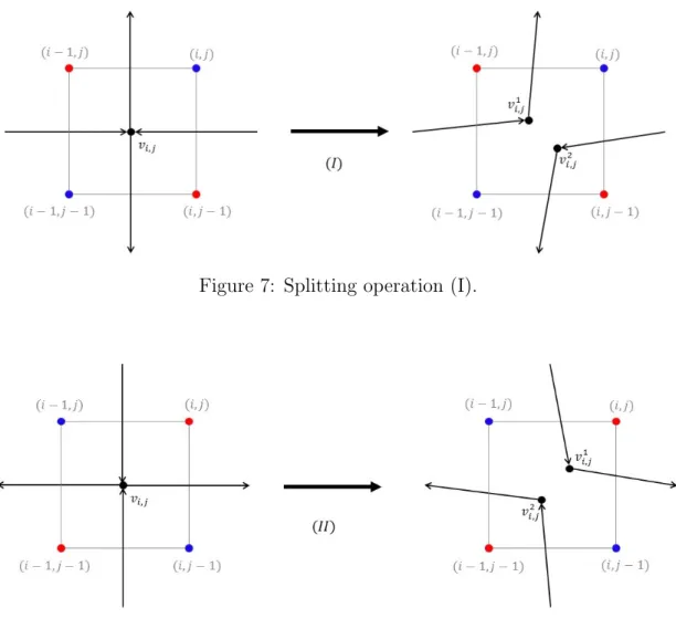
The difficulty of analyzing the approximation factor is due to the way the choice of K2 depends on the choice of K1. We overcome this difficulty by abandoning the minimum weight cuts K2 in favor of random ball cuts that are easier to analyze. To do this, we need to define two types of feasible solutions to (s, r, t)-Node-Lin-3-Cut. For 0< θ1 ≤1 and 0< θ2 ≤1, thevertical T-shaped cut V(θ1, θ2) is defined as
V(θ1, θ2) := Sout(r, θ1)∪(Bout(r, θ1)∩Sin(r, θ2)), while the horizontal T-shaped cut H(θ1, θ2) is defined as
H(θ1, θ2) := Sin(r, θ2)∪(Bin(r, θ2)∩Sout(r, θ1)).
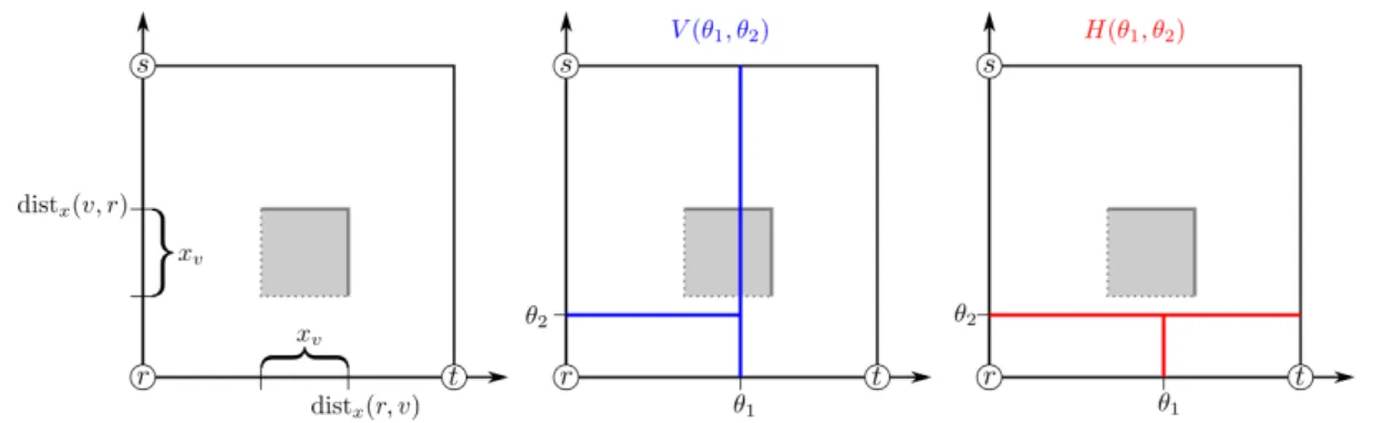
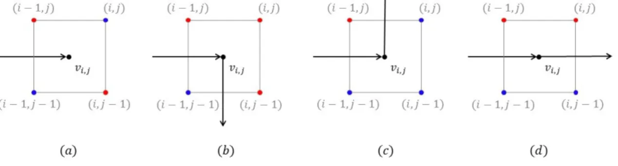
The name “T-shaped cut” comes from the observation that if each node v is repre- sented in the plane by the square (distx(r, v)−xv,distx(r, v)]×(distx(v, r)−xv,distx(v, r)], then the cut consists of nodes whose square is intersected by two segments forming a rotated “T” shape (see Figure 1).
Figure 1: Representation of T-shaped cuts. Left: the square corresponding to node v. Center: v is in V(θ1, θ2) because one of the blue lines intersects the square. Right:
v is not inH(θ1, θ2) because the red lines do not intersect the square.
Lemma 2.1. The set Bout(r, θ1)∩Sin(r, θ2)is an s→r cut in D[V \Sout(r, θ1)], and Bin(r, θ2)∩Sout(r, θ1) is an r→t cut in D[V \Sin(r, θ2)].
Proof. We prove only the first part of the claim, the proof of the second part being similar. Let us consider a path P ∈ Psr without any nodes in Sout(r, θ1). Let the nodes inP bew0 :=s, w1, w2, . . . , wk, wk+1 :=rappearing in order. We will show that wi ∈Bout(r, θ1) for everyi∈ {1, . . . , k}by induction on i. For the base case, owing to the presence of the edge r→s in the graph, we have that distx(r, w0)−xw0 = 0< θ1 and sincew0 6∈Sout(r, θ1), it follows that distx(r, w0)< θ1. For the induction step, we have thatdistx(r, wi+1)−xwi+1 ≤distx(r, wi)< θ1, where the second inequality follows by induction hypothesis. Now, since wi+1 6∈Sout(r, θ1), it follows thatdistx(r, wi+1)<
θ1. Hence, all nodes of P are in Bout(r, θ1).
We now show that at least one of the nodes in P should be in Sin(r, θ2). If distx(wi, r)< θ2 for everyi∈[k], thendistx(w1, r)< θ2 ≤1 and hence, distx(s, r)<1, a contradiction. Hence, there exists a node wi such that distx(wi, r) ≥ θ2. Pick the
node wi with the largest index i such that distx(wi, r) ≥ θ2. We have distx(wi, r)− xwi ≤ distx(wi+1, r) < θ2, where the second inequality is by the choice of the in- dex i. Thus, wi ∈ Sin(r, θ2) and hence, the path P contains a node in Sin(r, θ2).
Consequently, P contains a node inBout(r, θ1)∩Sin(r, θ2).
Corollary 2.1. Every T-shaped cut is a feasible solution to (s, r, t)-Node-Lin-3- Cut, and the weight of the cut found by the Deterministic Ball-Cut Algorithm is at most the minimum weight of a T-shaped cut.
Proof. Feasibility follows directly from Lemma 2.1 and Claim 2.2. For the second statement, consider V(θ1, θ2) for some θ1, θ2 ∈ (0,1]. By Claim 2.1, there exists θ0 ∈ {distx(r, v),distx(r, v)−xv} for some v ∈ V such that Sout(r, θ0) = Sout(r, θ1).
When the algorithm considers v and θ0, it finds a minimum weight s → r cut K2 in D[V \Sout(r, θ)]. As Bout(r, θ1)∩Sin(r, θ2) is also an s → r cut in D[V \Sout(r, θ)]
by Lemma 2.1, w(Sout(r, θ0)∪K2)≤w(Sout(r, θ1)∪(Bout(r, θ1)∩Sin(r, θ2)).
We can bound the approximation factor of Deterministic Ball-Cut Algorithm by estimating the minimum weight of a T-shaped cut. We show that this gives the desired factor of √
2.
Theorem 2.1. There exists a T-shaped cut U such that w(U)≤√ 2wTx.
To prove Theorem 2.1, we will follow a probabilistic argument. We will exhibit a distribution over T-shaped cuts for which the expected weight satisfies the bound mentioned in Theorem 2.1. This distribution turns out to be non-trivial in nature.
Instead of stating this distribution upfront and analyzing its approximation factor, we will derive the optimal distribution as a natural consequence of the following lemma, which provides a sufficient condition for achieving a certain approximation factor.
Lemma 2.2. Let ξ : [0,1]2 →R+ be a function satisfying Z 1
0
(ξ(a, z) +ξ(b, z)) dz+ Z 1
a
ξ(z, b) dz+ Z 1
b
ξ(z, a) dz = 1 ∀a, b∈R+, a+b ≤1.
(2) Let α := 2R1
0
R1
0 ξ(z1, z2) dz1dz2. Then, for any instance of (s, r, t)-Node-Lin-3- Cut, there exists a T-shaped cut U such that
w(U)≤ 1
α
wTx.
Proof. We define a probability distribution on the set of T-shaped cuts by giving a weighing functionf :{Ver,Hor}×[0,1]2 →R+. For (θ1, θ2)∈[0,1]2, letf(Ver, θ1, θ2) :=
ξ(θ1, θ2)/α and f(Hor, θ1, θ2) :=ξ(θ2, θ1)/α. For a T-shaped cut U, let Pr(U) :=
Z
(θ1,θ2):V(θ1,θ2)=U
f(Ver, θ1, θ2) dθ1dθ2+ Z
(θ1,θ2):H(θ1,θ2)=U
f(Hor, θ1, θ2) dθ1dθ2. We mention that a node setU could be both a horizontal and a vertical T-shaped cut in which case, the probability mass forU comes from both integrals in the above sum.
Furthermore Pr(·) is a probability distribution supported over the set of T-shaped cuts because of the definition of α. Let U be a T-shaped cut chosen according to this distribution.
Claim 2.3. For v ∈ V \ {r, s, t}, probability that v is in the chosen T-shaped cut U is at most xv/α.
Proof. We may assume that xv 6= 0 since every vertex in a T-shaped cut necessarily has this property. Leta:=distx(r, v) and b:=distx(v, r). We recall that a vertical T- shaped cutV(θ1, θ2) is defined asSout(r, θ1)∪(Bout(r, θ1)∩Sin(r, θ2)). Thus,V(θ1, θ2) contains the node v if and only if either (1) a−xv < θ1 ≤ a, or (2) a < θ1 and b−xv < θ2 ≤b. Similarly, a horizontal T-shaped cut H(θ1, θ2) contains the nodev if and only if either (3) b−xv < θ2 ≤b, or (4) b < θ2 and a−xv < θ1 ≤ a. Therefore the probability of v being in a random T-shaped cut is at most
P :=1 α
Z 1 z2=0
Z a z1=a−xv
ξ(z1, z2) dz1dz2+ Z b
z2=b−xv
Z 1 z1=a
ξ(z1, z2) dz1dz2 +
Z b z2=b−xv
Z 1 z1=0
ξ(z2, z1) dz1dz2+ Z 1
z2=b
Z a z1=a−xv
ξ(z2, z1) dz1dz2
By change of variables, we have that P = 1
α Z xv
y=0
Z 1 z=0
ξ(a−y, z) dz+ Z 1
z=a
ξ(z, b−xv +y) dz +
Z 1 z=0
ξ(b−xv+y, z) dz+ Z 1
z=b
ξ(z, a−y) dz
dy.
For 0 ≤ y ≤ xv, we have a−y ≤ a and b−xv +y ≤ b. By assumption, ξ(z1, z2) is non-negative in the domain. Therefore, we have
Z xv
y=0
Z 1 z=a
ξ(z, b−xv +y) dzdy≤ Z xv
y=0
Z 1 z=a−y
ξ(z, b−xv +y) dzdy, and Z xv
y=0
Z 1 z=b
ξ(z, a−y) dzdy≤ Z xv
y=0
Z 1 z=b−xv+y
ξ(z, a−y) dzdy.
Hence,
P ≤ 1 α
Z xv
y=0
Z 1 z=0
ξ(a−y, z) dz+ Z 1
z=a−y
ξ(z, b−xv +y) dz +
Z 1 z=0
ξ(b−xv+y, z) dz+ Z 1
z=b−xv+y
ξ(z, a−y) dz
dy
= 1 α
Z xv
y=0
1 dy = xv α,
where the equality at the beginning of the last row follows from (2), since for 0≤y≤ xv, we have (a−y) + (b−xv +y) =a+b−xv =distx(r, v) +distx(v, r)−xv ≤1 by (1), and moreover a−y ≥ a−xv = distx(r, v)−xv ≥ 0 and b−xv +y ≥ b−xv = distx(v, r)−xv ≥0 by the definition of distx(·,·).
Since every node v is in the random T-shaped cut with probability at most xαv, expected weight of a random T-shaped cut is at most wαTx. Therefore, there is a T-shaped cut U with w(U)≤ wαTx.
To prove the Theorem 2.1, it is enough by Lemma 2.2 to show the existence of a function ξ: [0,1]2 →R+ satisfying (2) for which
Z 1 0
Z 1 0
ξ(z1, z2) dz1dz2 = 1 2√
2. (3)
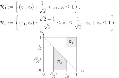
It turns out that such a function exists, but its structure is surprisingly complex. We define two regions where the function ξ will have positive values, see Figure 2.
R1 :=
(z1, z2) : 1
√2 < z1, z2 ≤1
,
R2 :=
(
(z1, z2) :
√2−1
√2 ≤z1 ≤ 1
√2, z1+z2 ≤1 )
.
Figure 2: The regions R1 and R2.
Remark. The reason for this restriction on the support of ξ will become apparent in Section 3, where we present an infinite sequence of node-weighted graphs for which the integrality gap of Distance-LP converges to √
2. It can be seen that R1 ∪ R2 consists of the pairs (z1, z2) for which the weight of the vertical T-shaped cutV(z1, z2) (based on the optimal LP solutionx) converges to 1 in the graph sequence. Informally, the regionR1∪ R2 is the region where the complementary slackness conditions allow positive density, if we consider the “limit” of the weighted graph sequence defined in Section 3. However, this is not the usual notion of graph limit, so we do not formalize this statement as it is not necessary for the proof.
Proof of Theorem 2.1. To prove the theorem, we define a function ξ with the above properties. The value ofξ is defined to be 0 for (z1, z2)∈[0,1]2\(R1∪ R2). For every (z1, z2)∈ R1, we set ξ(z1, z2) := (√
2 + 1)/√
2. In the regionR2, the value of ξ(z1, z2) will depend only on z1. In particular, we will define a function ζ : [
√√2−1 2 ,√1
2]→ R+, and define ξ(z1, z2) in the region R2 as
ξ(z1, z2) :=ζ(z1).
Let us examine the properties that must be satisfied by ζ in order for ξto satisfy (2).
Claim 2.4. Condition (2) is satisfied by ξ if the following hold for ζ:
ζ
√2−1
√2
!
= 0, (4)
(1−y)ζ(y) + Z 1−y
y
ζ(z) dz = 1 2 if
√2−1
√2 ≤y≤ 1
2, (5)
(1−y)ζ(y)− Z y
1−y
ζ(z) dz = 1 2 if 1
2 ≤y≤ 1
√2. (6)
Proof. We consider several cases based on the values of a and b. Let Γ(a, b) denote the LHS of (2). By taking y =
√√2−1
2 in (5) and substituting ζ(
√√2−1
2 ) = 0, we obtain that
Z √1
2
√√2−1 2
ζ(z) dz = 1
2. (7)
Case 1(i): Supposea > √1
2. Thenb ≤
√√2−1
2 since a+b ≤1. Now, Γ(a, b) =
Z 1 0
ξ(a, z) dz+ Z 1
0
ξ(b, z) dz+ Z 1
a
ξ(z, b) dz+ Z 1
b
ξ(z, a) dz
=
1 + 1
√2 1− 1
√2
+ 0 + 0 +
1 + 1
√2 1− 1
√2
= 1.
Case 1(ii): Supposeb > √1
2. Proceeding similar to Case 1(i), we obtain Γ(a, b) = 1.
Case 2: Suppose a≤
√√2−1
2 and b≤
√√2−1
2 . In this case, we have Γ(a, b) =
Z 1 0
ξ(a, z) dz+ Z 1
0
ξ(b, z) dz+ Z 1
a
ξ(z, b) dz+ Z 1
b
ξ(z, a) dz
= 0 + 0 + 2 Z √1
2
√
√2−1 2
ζ(z) dz = 1.
Case 3(i): Suppose
√√2−1
2 < a≤ √12 and b ≤
√√2−1
2 . Then Γ(a, b) =
Z 1 0
ξ(a, z) dz+ Z 1
0
ξ(b, z) dz+ Z 1
a
ξ(z, b) dz+ Z 1
b
ξ(z, a) dz
= Z 1−a
0
ζ(a) dz+ 0 + Z √1
2
a
ζ(z) dz+ Z 1−a
√√2−1 2
ζ(z) dz
= (1−a)ζ(a) + Z √1
2
a
ζ(z) dz+ Z 1−a
√
√2−1 2
ζ(z) dz. (8)
Ifa ≤ 12, then the RHS from (8) can be written as Γ(a, b) = (1−a)ζ(a) +
Z 1−a a
ζ(z) dz+ Z √1
2
√√2−1 2
ζ(z) dz = 1 by (5) and (7). Ifa > 12, then the RHS from (8) can be written as
Γ(a, b) = (1−a)ζ(a)− Z a
1−a
ζ(z) dz+ Z √1
2
√√2−1 2
ζ(z) dz = 1 by (6) and (7).
Case 3(ii): Suppose a ≤
√√2−1
2 and
√√2−1
2 < b ≤ √12. Proceeding similar to Case 3(a), we obtain that Γ(a, b) = 1.
Case 4: Suppose
√√2−1
2 < a≤ √12 and
√√2−1
2 < b≤ √12. Moreover, we havea+b ≤1.
Γ(a, b) = Z 1
0
ξ(a, z) dz+ Z 1
0
ξ(b, z) dz+ Z 1
a
ξ(z, b) dz+ Z 1
b
ξ(z, a) dz
= Z 1−a
0
ζ(a) dz+ Z 1−b
0
ζ(b) dz+ Z 1−b
a
ζ(z) dz+ Z 1−a
b
ζ(z) dz
= (1−a)ζ(a) + (1−b)ζ(b) + Z 1−b
a
ζ(z) dz+ Z 1−a
b
ζ(z) dz.
We will assume that a≤b (the other case is similar). If b≤ 12, then Z 1−b
a
ζ(z) dz+ Z 1−a
b
ζ(z) dz = Z 1−a
a
ζ(z) dz+ Z 1−b
b
ζ(z) dz,
and hence Γ(a, b) = 1 follows from (5). If b > 12, then, a ≤1−b < 12 ≤ b and hence, we have
Z 1−b a
ζ(z) dz+ Z 1−a
b
ζ(z) dz = Z 1−a
a
ζ(z) dz− Z b
1−b
ζ(z) dz.
Therefore, Γ(a, b) = 1 follows from (5) and (6).
We note that conditions (4)-(6) on ζ are actually necessary for (2) to hold. This fact is not needed for the proof of Theorem 2.1, but we prove it in Appendix A to facilitate future investigations on our distribution.
In order to complete the proof of the theorem, we have to find a function ζ : [
√√2−1
2 ,√12]→R+that satisfies properties (4)-(6). By solving the differential equations corresponding to (4)-(6), we get that the function satisfying these properties is
ζ(y) := 2y(2−y)−1
4y(1−y)2 . (9)
By substituting the function values, it can be verified that R1 0
R1
0 ξ(z1, z2) dz1dz2 =
1 2√
2. We present the calculations needed for verification in Appendix B.
For clarity, we conclude the section by describing the obtained distribution explic- itly. The probability of choosing a given T-shaped cutU is
Pr(U) := √ 2
Z
(θ1,θ2):V(θ1,θ2)=U
ξ(θ1, θ2) dθ1dθ2+ Z
(θ1,θ2):H(θ1,θ2)=U
ξ(θ2, θ1) dθ1dθ2
,
where
ξ(θ1, θ2) :=
√√2+1
2 if √1
2 < θ1, θ2 ≤1,
2θ1(2−θ1)−1 4θ1(1−θ1)2 if
√√2−1
2 ≤θ1 ≤ √12 and θ1+θ2 ≤1,
0 otherwise.
(10)
3 Integrality Gap
It is known that the inapproximability factor of (s, r, t)-Node-Lin-3-Cutunder UGC coincides with the integrality gap of theDistance-LP[4]. In this section, we present an integrality gap instance for (s, r, t)-Node-Lin-3-Cutwhich will in turn show the inapproximability result in Theorem 1.1.
Theorem 3.1. The integrality gap of the Distance-LP is at least √ 2.
We will construct a sequence of node-weighted graphs for which the integrality gap converges to √
2. In most previously known integrality gap instances for distance- based linear programs for directed multicut-like problems, the node weights were uniformly set to be one. In contrast, our gap instance assigns varying weights to the nodes.
3.1 Gap Instance Construction
Let M be a positive integer. We will construct a graph G= (V, E) on (M + 1)2 + 3 nodes with weights on the nodes. For convenience, let us define V0 :={(i, j) :i, j ∈ {0,1, . . . , M}}. Thus, we may viewV0 as the nodes of a (M+ 1)×(M+ 1)-grid whose columns and rows are indexed from 0 to M (we will follow the convention that the first index denotes the column while the second index denotes the row). The node set of G is given by V := {s, r, t} ∪V0. We now define the weights on the nodes.
The construction involves a parameterα ∈(0,1/2) that will be determined later. We denote the weight of node (i, j) to be wij and define6
wij :=
0 if i+j > M,
1−α
M if i+j < M,
1
2 −(1−α)iM if i+j =M, i < M
1− 2(1−α)1 ,
α if i+j =M, M
1− 2(1−α)1
≤i≤M
1 2(1−α)
, and
1
2 −(1−α)jM if i+j =M, i > M 1
2(1−α)
.
6The various boundary conditions in the definition of the node weights will have to use appropri- ately rounded down and rounded up boundary values. We avoid this technicality in the interests of simplicity.
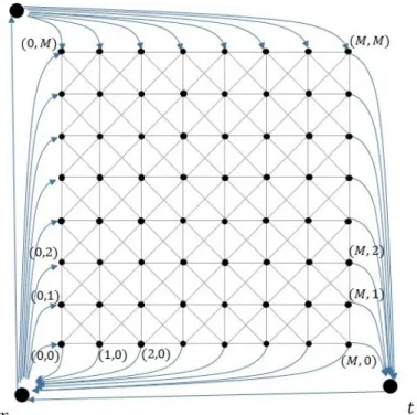
The edge setEconsists of undirected and directed edges. The undirected edges consist of the following: every node (i, j) is adjacent to all nodes in V0∩ {(i−1, j−1),(i− 1, j),(i−1, j+ 1),(i, j−1),(i, j+ 1),(i+ 1, j−1),(i+ 1, j),(i+ 1, j+ 1)}. The directed edges consist of r → s, t →r, s → (i, M) and (i,0)→ r for every i ∈ {0,1, . . . , M}, and (M, j)→t and r→(0, j) for every j ∈ {0,1. . . , M}. See Figure 3.
We will refer to the subgraph ofG induced by the vertex-set V0 as a diagonalized- grid. The leftmost column, rightmost column, bottommost row, topmost row, and diagonal refer to{(0, j) :j ∈ {0,1, . . . , M}}, {(M, j) :j ∈ {0,1, . . . , M}},{(i,0) :i∈ {0,1, . . . , M}}, {(i, M) : i ∈ {0,1, . . . , M}}, and {(i, j) : i, j ∈ {0,1, . . . , M}, i+j = M}respectively.
Figure 3: The graph corresponding to the integrality gap instance. The black edges are undirected while the blue edges are directed. The node weights are not shown.
3.2 Proof of Gap
The following lemma bounds the value of an optimal solution to the linear program.
Lemma 3.1. An optimal solution to the Distance-LP for the node-weighted graph constructed above has weight at most
1 M
M
X
i=0 M
X
j=0
wij.
Proof. It is sufficient to exhibit a feasible solution to the linear program whose ob- jective value is as specified in the lemma. We will show that x(i,j) := 1/M for every i, j ∈ {0,1, . . . , M}, i+j ≤M and x(i,j) := 1 for everyi, j ∈ {0,1, . . . , M}, i+j > M, is a feasible solution to the linear program. We recall that nodes (i, j) withi+j > M have weight wij = 0. Let us consider the graph H obtained from G by removing all nodes (i, j) with i+j > M. To show feasibility of x, it suffices to show that every path froms tor, fromr tot and froms tot has at leastM intermediate nodes inH.
A path in H from a node (i, j) ∈ V(H) to r has to cross j intermediate rows and hence has at least j internal nodes. Hence, for every node (i, j) with i, j ∈ {0,1. . . , M}, i+j ≤M, the number of internal nodes in every path from (i, j) to r in H is at least j. Now every path from s to r in H has to go through (0, M) and hence has at leastM internal nodes from V(H)∩V0. Similarly, every path from r to t inH has at least M internal nodes fromV(H)∩V0. Finally, the distance from s to t in H is at least the distance from r to t in H owing to the edge r →s and hence, the number of internal nodes fromV(H)∩V0 in any path froms to t inH is also at least M.
The next lemma shows a lower bound on the objective value of an integral optimum solution.
Lemma 3.2. An optimal solution to (s, r, t)-Node-Lin-3-Cut in the node-weighted graph constructed above has weight at least 1.
Proof. LetU∗ be an integral optimal solution. We will show the lower bound on the weight of U∗ in two steps. We define the axis-parallel neighbors of a node (i, j) to be the nodes in {(i+ 1, j),(i−1, j),(i, j + 1),(i, j −1)} and a path to be an axis- parallel path if all neighbors of a node (i, j) occurring in the path are its axis-parallel neighbors. In the first step of the proof, we will show that U∗ consists of an axis- parallel path from a node in the topmost row to a node in the bottommost row and an axis-parallel path from a node in the leftmost column to a node in rightmost column.
In the second step of the proof, we will show a lower bound on the total weight of the union of the nodes in these two paths.
Lemma 3.3. The optimal solution U∗ contains a set of nodes which form an axis- parallel path P1 from a node in the bottommost row to a node in the topmost row in G.
Lemma 3.4. The optimal solution U∗ contains a set of nodes which form an axis- parallel path P2 from a node in the leftmost column to a node in the rightmost column in G.
We defer the proof of Lemmas 3.3 and 3.4 and proceed with the proof of Lemma 3.2. The next claim follows immediately from the definition of axis-parallel paths.
Claim 3.1. Every axis-parallel path from node (i1, j1) to (i2, j2) contains at least
|i2−i1|+|j2−j1| −1 internal nodes.
We also have the following claim from the definition of the node weights.
Claim 3.2. For every node (i, j) for i, j ∈ {0,1, . . . , M} with i+j =M, we have wij = max
1
2 −(1−α)i M , α,1
2− (1−α)j M
.
Let P1 and P2 be the node sets guaranteed by Lemmas 3.3 and 3.4 respectively.
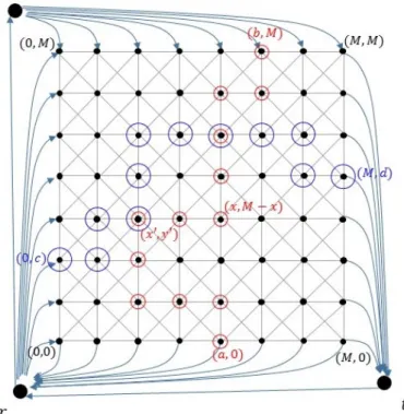
Without loss of generality, let P1 be the node set in U∗ that induces an axis-parallel path from a node (a,0) to a node (b, M). Similarly, letP2 be the node set in U∗ that induces an axis-parallel path from a node (0, c) to a node (M, d) (see Figure 4).
Figure 4: The red circled nodes denote the axis-parallel path P1 and the blue circled nodes denote the axis-parallel path P2.
SinceP1 is an axis-parallel path from a node in the bottommost row to a node in the topmost row, there exists a node inP1 from the diagonal. Let (x, M−x) be the first node along the axis-parallel pathP1 that is in the diagonal. Let P10 be the restriction of P1 from (a,0) to (x, M −x). Let (x0, y0) be the first node along the axis-parallel path P2 that is either in the diagonal or in P10. Let P20 be the restriction of P2 from (0, c) to (x0, y0). By construction, all nodes (p, q) of P10 ∪P20 satisfy p+q ≤ M. We will show that the total weight of the nodes inP10∪P20 is at least 1. This suffices since P10∪P20 ⊆U∗. We distinguish two cases.
1. Suppose P20 is a path from (0, c) to a node (i, j) of P10, where i+j ≤ M. By Claim 3.1, the axis-parallel pathP20 has at least|i−0|+|j−c|−1≥i−1 internal nodes. Furthermore, the path P10 is the concatenation of an axis-parallel path Q1 from (a,0) to (i, j) and an axis-parallel path Q2 from (i, j) to (x, M −x).
Hence, by Claim 3.1, the axis-parallel pathP10 has at least |i−a|+|j−0| −1 + 1 +|x−i|+|M−x−j| −1≥j+|x−i|+|M−x−j| −1≥M−i−1 internal nodes. We recall that all these nodes have weight (1−α)/M. Additionally, the nodes (a,0) and (0, c) have weight (1−α)/M each. The node (x, M−x) on the diagonal has weight at least α by Claim 3.2. Combining these, we get that the total weight of the nodes inP10 ∪P20 is at least
((i−1) + (M −i−1) + 2)
1−α M
+α= 1.
2. Suppose P20 is a path from (0, c) to a node (x0, M − x0) on the diagonal. In this case, we will show that the total weight of the nodes in P10 and P20 are each lower bounded by 1/2. By Claim 3.1, the axis-parallel path P10 has at least
|x−a|+|M −x−0| −1≥M−x−1 internal nodes each of which has weight (1−α)/M. Additionally, the end-node (a,0) also has weight (1−α)/M and the end-node (x, M −x) has weight at least 1/2−(1−α)((M −x)/M) by Claim 3.2. Thus, the total weight of the nodes inP10 is at least
((M −x−1) + 1)
1−α M
+1
2 − (1−α)(M −x)
M = 1
2.
We proceed by a similar argument for the total weight of the nodes in P20. By Claim 3.1, the axis-parallel pathP20 has at least|x0−0|+|M−x0−c| −1≥x0−1 internal nodes each of which has weight (1−α)/M. Additionally, the end-node (0, c) also has weight (1−α)/M and the end-node (x0, M −x0) has weight at least 1/2−(1−α)(x0/M) by Claim 3.2. Thus, the total weight of the nodes in P20 is at least
((x0−1) + 1)
1−α M
+1
2 −(1−α)x0
M = 1
2. This completes the proof of Lemma 3.2.
We now prove Lemma 3.3. The proof of Lemma 3.4 is similar.
Proof of Lemma 3.3. LetUt∗ denote an inclusionwise-minimal subset ofU∗ such that G−Ut∗ contains no path from r to t. We will show that Ut∗ contains a path P1 as required. Showing this is equivalent to showing the following combinatorial statement:
every subset of nodes that intersects all paths from left to right in a diagonalized-grid (since G contains a diagonalized-grid) has a subset of nodes that induce an axis- parallel path from a node in the topmost row to a node in the bottommost row in G.
We proceed to show this now.
We will show the combinatorial statement using a coloring argument. Let R :=Ut∗∪ {(i,−1),(i, M + 1) :i∈ {0,1, . . . , M}} and
B := (V0\Ut∗)∪ {(−1, j),(M + 1, j) :j ∈ {0,1, . . . , M}}.
and call the corresponding nodes as red and blue nodes respectively (we observe that the sets R and B have extra nodes in addition to the nodes in the diagonalized-grid of G, but this is only for the purposes of notational convenience in this proof). We will construct an auxiliary graph for the purposes of the proof—for clarity, we will refer to the vertices ofG asnodes and the vertices of the auxiliary graph asvertices.
We construct an undirected graph H as follows. The vertex set of H is given by V(H) := {vi,j : i, j ∈ {0,1, . . . , M + 1}} ∪ {a, b, c, d}. We call a vertex vi,j to be in column i and row j. We define a0 := v0,0, b0 := vM+1,0, c0 := v0,M+1, d0 := vM+1,M+1 and call them to be the corner vertices.
The edge set of H is denoted by E(H): a vertex vi,j is adjacent to all vertices in V(H)∩{vi−1,j, vi+1,j, vi,j−1, vi,j+1}(i.e., the undirected grid edges) and verticesa, b, c, d are adjacent to a0, b0, c0, d0 respectively.
We note that H is a plane graph that corresponds to a square grid with four pendant vertices that are adjacent to the four corner vertices of the grid. In the following, it is helpful to consider overlaying H on top of G as shown in Figure 5 with each internal face of H containing exactly one node from V0. For a vertex vi,j ∈V(H)\ {a, a0, b, b0, c, c0, d, d0}, we defineD1i,j :={(i, j),(i−1, j−1)} andDi,j2 :=
{(i−1, j),(i, j −1)}. We emphasize that D1i,j and D2i,j consist of nodes from the original graph G. They are the nodes in the two diagonally opposite faces adjacent tovi,j in the overlay (see Figure 5).
Figure 5: The diagonalized-grid of the graph G is shown in gray while the graph H is shown in black. For visual simplicity, we have not included the diagonal edges of the diagonalized-grid. The extra red and blue nodes are also shown. For node vi,j, the nodes ofG in the two diagonally opposite faces D1i,j and Di,j2 are also shown.