Egerv´ ary Research Group
on Combinatorial Optimization
Technical reportS
TR-2019-04. Published by the Egerv´ary Research Group, P´azm´any P. s´et´any 1/C, H–1117, Budapest, Hungary. Web site: www.cs.elte.hu/egres. ISSN 1587–4451.
Improving the Integrality Gap for Multiway Cut
Krist´ of B´erczi, Karthekeyan Chandrasekaran, Tam´ as Kir´ aly, and Vivek Madan
March 2019
EGRES Technical Report No. 2019-04 1
Improving the Integrality Gap for Multiway Cut
Krist´ of B´ erczi
?, Karthekeyan Chandrasekaran
??, Tam´ as Kir´ aly, and Vivek Madan
Abstract
In the multiway cut problem, we are given an undirected graph with non- negative edge weights and a collection ofk terminal nodes, and the goal is to partition the node set of the graph into k non-empty parts each containing exactly one terminal so that the total weight of the edges crossing the partition is minimized. The multiway cut problem fork≥3 is APX-hard. For arbitrary k, the best-known approximation factor is 1.2965 due to Sharma and Vondr´ak [11] while the best known inapproximability factor is 1.2 due to Angelidakis, Makarychev and Manurangsi [1]. In this work, we improve on the lower bound to 1.20016 by constructing an integrality gap instance for the CKR relaxation.
A technical challenge in improving the gap has been the lack of geometric tools to understand higher-dimensional simplices. Our instance is a non-trivial 3-dimensional instance that overcomes this technical challenge. We analyze the gap of the instance by viewing it as a convex combination of 2-dimensional instances and a uniform 3-dimensional instance. We believe that this technique could be exploited further to construct instances with larger integrality gap.
One of the ingredients of our proof technique is a generalization of a result on Sperner admissible labelings due to Mirzakhani and Vondr´ak [10] that might be of independent combinatorial interest.
Keywords: Combinatorial optimization, Multiway cut, Integrality gap, Ap- proximation
?MTA-ELTE Egerv´ary Research Group, Department of Operations Research, E¨otv¨os Lor´and University, Budapest, Email: {berkri,tkiraly}@cs.elte.hu.
??University of Illinois, Urbana-Champaign, Email: {karthe,vmadan2}@illinois.edu. Vivek is supported by the NSF grant CCF-1319376.
Section 1. Introduction 2
1 Introduction
In the multiway cut problem, we are given an undirected graph with non-negative edge weights and a collection of k terminal nodes and the goal is to find a minimum weight subset of edges to delete so that thekinput terminals cannot reach each other.
For convenience, we will use k-way cut to denote this problem when we would like to highlight the dependence on k and multiway cut to denote this problem when k grows with the size of the input graph. The 2-way cut problem is the classic mini- mum {s, t}-cut problem which is solvable in polynomial time. For k ≥3, Dahlhaus, Johnson, Papadimitriou, Seymour and Yannakakis [6] showed that the k-way cut problem is APX-hard and gave a (2−2/k)-approximation. Owing to its applications in partitioning and clustering, k-way cut has been an intensely investigated problem in the algorithms literature. Several novel rounding techniques in the approximation literature were discovered to address the approximability of this problem.
The known approximability as well as inapproximability results are based on a linear programming relaxation, popularly known as the CKR relaxation in honor of the authors—C˘alinescu, Karloff and Rabani—who introduced it [4]. The CKR relaxation takes a geometric perspective of the problem. For a graphG= (V, E) with edge weightsw:E →R+ and terminals t1, . . . , tk, the CKR relaxation is given by
min 1 2
X
e={u,v}∈E
w(e)kxu−xvk1 xu ∈∆k ∀ u∈V,
xti =ei ∀ i∈[k], where ∆k :={(x1, . . . , xk)∈[0,1]k : Pk
i=1xi = 1} is the (k−1)-dimensional simplex and ei ∈ {0,1}k is the extreme point of the simplex along the i-th coordinate axis, i.e., eij = 1 if and only if j =i.
C˘alinescu, Karloff and Rabani designed a rounding scheme for the relaxation which led to a (3/2−1/k)-approximation thus improving on the (2−2/k)-approximation by Dahlhaus et al. For 3-way cut, Cheung, Cunningham and Tang [5] as well as Karger, Klein, Stein, Thorup and Young [8] designed alternative rounding schemes that led to a 12/11-approximation factor and also exhibited matching integrality gap instances. We recall that the integrality gap of an instance to the LP is the ratio between the integral optimum value and the LP optimum value. Determining the exact integrality gap of the CKR relaxation for k ≥ 4 has been an intriguing open question. After the results by Karger et al. and Cunningham et al., a rich variety of rounding techniques were developed to improve the approximation factor ofk-way cut for k ≥ 4 [2, 3, 11]. The known approximation factor for multiway cut is 1.2965 due to Sharma and Vondr´ak [11].
On the hardness of approximation side, Manokaran, Naor, Raghavendra and Schwartz [9] showed that the hardness of approximation for k-way cut is at least the integrality gap of the CKR relaxation assuming the Unique Games Conjecture (UGC). More precisely, if the integrality gap of the CKR relaxation for k-way cut is τk, then it is UGC-hard to approximate k-way cut within a factor of τk − for
Section 2. Background and Result 3
every constant > 0. As an immediate consequence of this result, we know that the 12/11-approximation factor for 3-way cut is tight. For k-way cut, Freund and Karloff [7] constructed an instance showing an integrality gap of 8/(7 + (1/(k−1))).
This was the best known integrality gap until last year when Angelidakis, Makarychev and Manurangsi [1] gave a remarkably simple construction showing an integrality gap of 6/(5 + (1/(k−1))) for k-way cut. In particular, this gives an integrality gap of 1.2 for multiway cut.
We note that the known upper and lower bounds on the approximation factor for multiway cut match only up to the first decimal digit and thus the approximability of this problem is far from resolved. Indeed Angelidakis, Makarychev and Manurangsi raise the question of whether the lower bound can be improved. In this work, we improve on the lower bound by constructing an instance with integrality gap 1.20016.
Theorem 1.1. For every constant >0, there exists an instance of multiway cut such that the integrality gap of the CKR relaxation for that instance is at least 1.20016−. The above result in conjunction with the result of Manokaran et al. immediately implies that multiway cut is UGC-hard to approximate within a factor of 1.20016− for every constant >0.
One of the ingredients of our technique underlying the proof of Theorem 1.1 is a generalization of a result on Sperner admissible labelings due to Mirzakhani and Vondr´ak [10] that might be of independent combinatorial interest (see Theorem 5.2).
2 Background and Result
Before outlining our techniques, we briefly summarize the background literature that we build upon to construct our instance. We rely on two significant results from the literature. In the context of thek-way cut problem, acut is a functionP : ∆k →[k+1]
such thatP(ei) =i for alli∈[k], where we use the notation [k] :={1,2, . . . , k}. The use of k+ 1 labels as opposed to k labels to describe a cut is a bit non-standard, but is useful for reasons that will become clear later on. The approximation ratio τk(P) of a distribution P over cuts is given by its maximum density:
τk(P) := sup
x,y∈∆k,x6=y
PrP∼P(P(x)6=P(y)) (1/2)kx−yk1 . Karger et al. [8] define
τk∗ := inf
P τk(P),
and moreover showed that there exists P that achieves the infimum. Hence, τk∗ = minPτk(P). With this definition of τk∗, Karger et al. [8] showed that for every > 0, there is an instance of multiway cut with k terminals for which the integrality gap of the CKR relaxation is at leastτk∗−. Thus, Karger et al.’s result reduced the problem of constructing an integrality gap instance for multiway cut to proving a lower bound onτk∗.
Section 3. Outline of Ideas 4
Next, Angelidakis, Makarychev and Manurangsi [1] reduced the problem of lower bounding τk∗ further by showing that it is sufficient to restrict our attention to non- opposite cuts as opposed to all cuts. A cut P is a non-opposite cut if P(x) ∈ Support(x)∪ {k + 1} for every x ∈ ∆k. Let ∆k,n := ∆k ∩((1/n)Z)k. For a dis- tribution P over cuts, let
τk,n(P) := max
x,y∈∆k,n,x6=y
PrP∼P(P(x)6=P(y)) (1/2)kx−yk1
, and
˜
τk,n∗ := min{τk,n(P) :P is a distribution over non-opposite cuts}.
Angelidakis, Makarychev and Manurangsi showed that ˜τk,n∗ −τK∗ =O(kn/(K−k)) for allK > k. Thus, in order to lower boundτK∗, it suffices to lower bound ˜τk,n∗ . That is, it suffices to construct an instance that has large integrality gap against non-opposite cuts.
As a central contribution, Angelidakis, Makarychev and Manurangsi constructed an instance showing that ˜τ3,n∗ ≥ 1.2−O(1/n). Now, by setting n = Θ(√
K), we see that τK∗ is at least 1.2−O(1/√
K). Furthermore, they also showed that their lower bound on ˜τ3,n∗ is almost tight, i.e., ˜τ3,n∗ ≤1.2. The salient feature of this framework is that in order to improve the lower bound on τK∗, it suffices to improve ˜τk,n∗ for some 4≤k < K.
The main technical challenge towards improving ˜τ4,n∗ is that one has to deal with the 3-dimensional simplex ∆4. Indeed, all known gap instances including that of Angelidakis, Makarychev and Manurangsi are constructed using the 2-dimensional simplex. In the 2-dimensional simplex, the properties of non-opposite cuts are easy to visualize and their cut-values are convenient to characterize using simple geometric observations. However, the values of non-opposite cuts in the 3-dimensional simplex become difficult to characterize. Our main contribution is a simple argument based on properties of lower-dimensional simplices that overcomes this technical challenge. We construct a 3-dimensional instance that has gap larger than 1.2 against non-opposite cuts.
Theorem 2.1. τ˜4,n∗ ≥1.20016−O(1/n).
Theorem 1.1 follows from Theorem 2.1 using the above arguments.
3 Outline of Ideas
Let G = (V, E) be the graph with node set ∆4,n and edge set E4,n := {xy : x, y ∈
∆4,n,kx−yk1 = 2/n}, where the terminals are the four unit vectors. In order to lower bound ˜τ4,n∗ , we will come up with weights on the edges of G such that every non-opposite cut has cost at least α = 1.20016 and moreover the cumulative weight of all edges isn+O(1). This suffices to lower bound ˜τ4,n∗ by the following proposition.
Proposition 3.1. Suppose that there exist weights w:E4,n →R≥0 on the edges of G such that every non-opposite cut has cost at least α and the cumulative weight of all edges is n+O(1). Then, τ˜4,n∗ ≥α−O(1/n).
Section 3. Outline of Ideas 5
Proof. For an arbitrary distribution P over non-opposite cuts, we have τk,n(P) = max
x,y∈∆k,n,x6=y
PrP∼P(P(x)6=P(y)) (1/2)kx−yk1
≥ max
xy∈E4,n
PrP∼P(P(x)6=P(y)) (1/2)kx−yk1
= max
xy∈E4,n
PrP∼P(P(x)6=P(y)) 1/n
≥ X
xy∈E4,n
w(xy)PrP∼P(P(x)6=P(y)) (1/n)(P
e∈E4,nw(e))
≥ α
1 +O(1/n) =α−O(1/n),
where the last inequality follows from the hypothesis that every non-opposite cut has cost at leastα and the cumulative weight of all edges is n+O(1).
We obtain our weighted instance from four instances that have large gap against different types of cuts, and then compute the convex combination of these instances that gives the best gap against all non-opposite cuts.
All of our four instances are defined as edge-weights on the graph G= (V, E). We identify ∆3,n with the facet of ∆4,n defined by x4 = 0. Our first three instances are 2-dimensional instances, i.e. only edges induced by ∆3,n have positive weight. The fourth instance has uniform weight onE4,n.
We first explain the motivation behind Instances 1,2, and 4, since these are easy to explain. Let
Lij :={xy∈E4,n : Support(x),Support(y)⊆ {i, j}}.
• Instance 1 is simply the instance of Angelidakis, Makarychev and Manurangsi [1]
on ∆3,n. It has gap 1.2− n1 against all non-opposite cuts, since non-opposite cuts in ∆4,n induce non-opposite cuts on ∆3,n. Additionally, we show in Lemma 4.5 that the gap is strictly larger than 1.2 by a constant if the following two conditions hold:
– there exist i, j ∈[3] such thatLij contains only one edge whose end-nodes have different labels (a cut with this property is called a non-fragmenting cut), and
– ∆3,n has a lot of nodes with label 5.
• Instance 2 has uniform weight on L12, L13 and L23, and 0 on all other edges.
Here, a cut in which eachLij contains at least two edges whose end-nodes have different labels (afragmenting cut) has large weight. Consequently, this instance has gap at least 2 against such cuts.
• Instance 4 has uniform weight on all edges in E4,n. A beautiful result due to Mirzakhani and Vondr´ak [10] implies that non-opposite cuts with no node of
Section 4. A3-dimensional gap instance against non-opposite cuts 6
label 5 have large weight. Consequently, this instance has gap at least 3/2 against such cuts. We extend their result in Lemma 4.4 to show that the weight remains large if ∆3,n has few nodes with label 5.
At first glance, the arguments above seem to imply that a convex combination of these three instances already gives a gap strictly larger than 1.2 for all non-opposite cuts. However, there exist two non-opposite cuts such that at least one of them has cost at most 1.2 in every convex combination of these three instances (see Section 7.1). One of these two cuts is a fragmenting cut that has almost zero cost in Instance 4 and the best possible cost, namely 1.2, in Instance 1. Instance 3 is constructed specifically to boost the cost against this non-opposite cut. It has positive uniform weight on 3 equilateral triangles, incident toe1,e2 ande3on the face ∆3,n. We call the edges of these triangles red edges. The side length of these triangles is a parameter, denoted by c, that is optimized at the end of the proof. Essentially, we show that if a non-opposite cut has small cost both on Instance 1 and Instance 4 (i.e., weight 1.2 on Instance 1 and O(1/n2) weight on Instance 4), then it must contain red edges.
Our lower bound of 1.20016 is obtained by optimizing the coefficients of the convex combination and the parameterc. By Proposition 3.1 and the results of Angelidakis, Makarychev and Manurangsi, we obtain that τK∗ ≥ 1.20016− O(1/√
K), i.e., the integrality gap of the CKR relaxation for k-way cut is at least 1.20016−O(1/√
k).
We complement our lower bound of 1.20016 by also showing that the best possible gap that can be achieved using convex combinations of our four instances is 1.20067 (see Section 7.2).
4 A 3-dimensional gap instance against non-oppo- site cuts
We will focus on the graph G = (V, E) with the node set V := ∆4,n being the discretized 3-dimensional simplex and the edge setE4,n :={xy :x, y ∈∆4,n,kx−yk1 = 2/n}. The four terminals s1, . . . , s4 will be the four extreme points of the simplex, namely si =ei for i ∈[4]. In this context, a cut is a function P :V →[5] such that P(si) =i for all i∈[4]. The cut-set corresponding to P is defined as
δ(P) :={xy∈E4,n :P(x)6=P(y)}.
For a set S of nodes, we will also use δ(S) to denote the set of edges with exactly one end node in S. Given a weight function w : E4,n → R+, the cost of a cut P is P
e∈δ(P)w(e). Our goal is to come up with weights on the edges so that the resulting 4-way cut instance has gap at least 1.20016 against non-opposite cuts.
We recall that Lij denotes the boundary edges between terminals si and sj, i.e., Lij ={xy∈E4,n: Support(x),Support(y)⊆ {i, j}}.
We will denote the boundary nodes between terminalssi and sj as Vij, i.e., Vij :={x∈∆4,n : Support(x)⊆ {i, j}}.
4.1 Gap instance as a convex combination 7
s1
s2 s3
L31 L12
L23
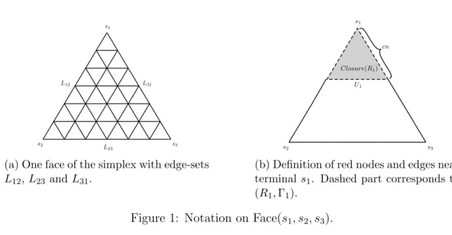
(a) One face of the simplex with edge-sets L12,L23 and L31.
s1
s2 s3
cn
Closure(R1) U1
(b) Definition of red nodes and edges near terminals1. Dashed part corresponds to (R1,Γ1).
Figure 1: Notation on Face(s1, s2, s3).
Let c ∈ (0,1/2) be a constant to be fixed later, such that cn is integral. For each k∈[3], we define node sets Uk, Rk and Closure(Rk) and edge set Γk as follows:
Uk :={x∈∆4,n :x4 = 0, xk = 1−c}, Rk :=Uk∪ {x∈Vik∪Vjk :xk ≥1−c}, Closure(Rk) :={x∈∆4,n :x4 = 0, xk ≥1−c}, and
Γk :={xy∈E4,n :x, y ∈Rk}.
We will refer to the nodes in Rk as red1 nodes near terminal sk and the edges in Γk as the red edges near terminal sk (see Figure 1b). Let Face(s1, s2, s3) denote the subgraph of G induced by the nodes whose support is contained in {1,2,3}. We emphasize that red edges and red nodes are present only in Face(s1, s2, s3) and that the total number of red edges is exactly 9cn.
4.1 Gap instance as a convex combination
Our gap instance is a convex combination of the following four instances.
1. Instance I1. Our first instance constitutes the 3-way cut instance constructed by Angelidakis, Makarychev and Manurangsi [1] that has gap 1.2 against non- opposite cuts. To ensure that the total weight of all the edges in their instance is exactly n, we will scale their instance by 6/5. Let us denote the resulting instance asJ. InI1, we simply use the instanceJ on Face(s1, s2, s3) and set the weights of the rest of the edges inE4,n to be zero.
2. Instance I2. In this instance, we set the weights of the edges in L12, L23, L13 to be 1/3 and the weights of the rest of the edges inE4,n to be zero.
1We use the term “red” as a convenient way for the reader to remember these nodes and edges.
The exact color is irrelevant.
4.2 Gap of the Convex Combination 8
3. Instance I3. In this instance, we set the weights of the red edges to be 1/9c and the weights of the rest of the edges in E4,n to be zero.
4. Instance I4. In this instance, we set the weight of every edge in E4,n to be 1/n2.
We note that the total weight of all edges in each of the above instances isn+O(1).
For multipliersλ1, . . . , λ4 ≥0 to be chosen later that will satisfy P4
i=1λi = 1, let the instance I be the convex combination of the above four instances, i.e., I = λ1I1 + λ2I2+λ3I3+λ4I4. By the properties of the four instances, it immediately follows that the total weight of all edges in the instance I is also n+O(1).
4.2 Gap of the Convex Combination
The following theorem is the main result of this section.
Theorem 4.1. For every n ≥ 10 and c ∈ (0,1/2) such that cn is integer, every non-opposite cut on I has cost at least the minimum of the following two terms:
(i) λ2+ (1.2− 1n)λ1+ minα∈[0,12]
0.4αλ1+ 3 12 −α λ4
(ii) 2λ2+ (1.2−2n5 )λ1+ 3 min
2λ3
9c,minα∈h
0,c22 i
n
0.4αλ1+ 3
c2 2 −α
λ4o
Before proving Theorem 4.1, we see its consequence.
Corollary 4.2. There exist constantsc∈(0,1/2)andλ1, λ2, λ3, λ4 ≥0withP4
i=1λi = 1 such that the cost of every non-opposite cut in the resulting convex combination I is at least 1.20016−O(1/n).
Proof. The corollary follows from Theorem 4.1 by setting λ1 = 0.751652, λ2 = 0.147852, λ3 = 0.000275, λ4 = 0.100221 and c= 0.074125 (this is the optimal setting to achieve the largest lower bound based on Theorem 4.1).
Corollary 4.2 in conjunction with Proposition 3.1 immediately implies Theorem 2.1.
The following theorem (shown in Section 7.2) complements Corollary 4.2 by giv- ing an upper bound on the best possible gap that is achievable using the convex combination of our four instances.
Theorem 4.3. For every constant c ∈ (0,1/2) and every λ1, λ2, λ3, λ4 ≥ 0 with P4
i=1λi = 1, there exists a non-opposite cut whose cost in the resulting convex com- bination I is at most 1.20067 +O(1/n).
In light of Corollary 4.2 and Theorem 4.3, if we believe that the integrality gap of the CKR relaxation is more than 1.20067, then considering convex combination of alternative instances is a reasonable approach towards proving this.
The rest of the section is devoted to proving Theorem 4.1. We rely on two main ingredients in the proof. The first ingredient is a statement about non-opposite cuts in the 3-dimensional discretized simplex. We prove this in Section 5, where we also give a generalization to higher dimensional simplices, which might be of independent interest.
4.2 Gap of the Convex Combination 9
Lemma 4.4. Let P be a non-opposite cut on ∆4,n with α(n+ 1)(n+ 2) nodes from Face(s1, s2, s3)labeled as 1, 2, or3 for some α∈[0,1/2]. Then, |δ(P)| ≥3αn(n+ 1).
The constant 3 that appears in the conclusion of Lemma 4.4 is the best possible for any fixedα (if n→ ∞). To see this, consider the non-opposite cut P obtained by labeling si to bei for every i∈[4], all nodes at distance at most αn froms1 to be 1, and all remaining nodes to be 5. The number of nodes from Face(s1, s2, s3) labeled as 1, 2, or 3 is αn2+O(n). The number of edges in the cut is 3αn2+O(n).
The second ingredient involves properties of the 3-way cut instance constructed by Angelidakis, Makarychev and Manurangsi [1]. We need two properties that are summarized in Lemma 4.5 and Corollary 4.2. We prove these properties in Section 6.
We define a cut Q: ∆3,n → [4] to be a fragmenting cut if |δ(Q)∩Lij| ≥2 for every distinct i, j ∈ [3]; otherwise it is a non-fragmenting cut. We recall that J denotes the instance obtained from the 3-way cut instance of Angelidakis, Makarychev and Manurangsi by scaling it up by 6/5.
The first property is that non-opposite non-fragmenting cuts in ∆3,n that label a large number of nodes with label 4 have cost much larger than 1.2.
Lemma 4.5. Let Q : ∆3,n → [4] be a non-opposite cut with αn2 nodes labeled as 4. If Q is a non-fragmenting cut and n ≥ 10, then the cost of Q on J is at least 1.2 + 0.4α−n1.
We show Lemma 4.5 by modifyingQto obtain a non-opposite cutQ0while reducing its cost by 0.4α. By the main result of [1], the cost of every non-opposite cutQ0 onJ is at least 1.2−n1. Therefore, it follows that the cost ofQonJ is at least 1.2−n1+0.4α.
We emphasize that while it might be possible to improve the constant 0.4 that appears in the conclusion of Lemma 4.5, it does not lead to much improvement on the overall integrality gap as illustrated by the results in Section 7.2.
The second property is that non-opposite cuts which do not remove any of the red edges, but label a large number of nodes in the red region with label 4 have cost much larger than 1.2. Let Q : ∆3,n → [4] be a non-opposite cut and n ≥ 10. For each i∈[3], let
Ai :=
({v ∈Closure(Ri) :Q(v) = 4} if δ(Q)∩Γi =∅,
∅ otherwise.
Then, the cost of Q onJ is at least 1.2 + 0.4P3
i=1|Ai|/n2−2n5 .
In order to show Corollary 4.2, we first derive that the cost of the edges δ(∪3i=1Ai) in the instanceJ is at least 0.4P3
i=1|Ai|/n2−2n3 using Lemma 4.5. Next, we modify Q to obtain a non-opposite cut Q0 such that δ(Q0) =δ(Q)\δ(∪3i=1Ai). By the main result of [1], the cost of every non-opposite cut Q0 onJ is at least 1.2−1n. Therefore, it follows that the cost ofQ on J is at least 1.2 + 0.4P3
i=1|Ai|/n2. We now have the ingredients to prove Theorem 4.1.
Proof of Theorem 4.1. LetP : ∆4,n →[5] be a non-opposite cut. LetQ be the cut P
4.2 Gap of the Convex Combination 10
restricted to Face(s1, s2, s3), i.e., for every v ∈∆4,n with Support(v)⊆[3], let Q(v) :=
(P(v) if P(v)∈ {1,2,3}, 4 if P(v) = 5.
We consider two cases.
Case 1: Qis a non-fragmenting cut. Let the number of nodes in Face(s1, s2, s3) that are labeled byQas 4 (equivalently, labeled byP as 5) beα(n+ 1)(n+ 2) for some α ∈
0,12
. Since |{x ∈ Face(s1, s2, s3) : Q(x) = 4}| ≥ αn2, Lemma 4.5 implies that the cost ofQonJ, and hence the cost ofP onI1, is at least 1.2 + 0.4α−n1. Moreover, the cost of P on I2 is at least 1 since at least one edge in Lij should be in δ(P) for every pair of distincti, j ∈[3]. To estimate the cost onI4, we observe that the number of nodes on Face(s1, s2, s3) labeled by P as 1, 2, or 3 is (1/2−α)(n+ 1)(n+ 2). By Lemma 4.4, we have that |δ(P)| ≥ 3(1/2−α)n(n+ 1) and thus, the cost of P onI4 is at least 3(1/2−α). Therefore, the cost of P on the convex combination instanceI is at least
λ2 +
1.2− 1 n
λ1+ min
α∈[0,12]
0.4αλ1+ 3 1
2 −α
λ4
.
Case 2: Q is a fragmenting cut. Then, the cost of P on I2 is at least 2 as a fragmenting cut contains at least 2 edges from eachLij for distinct i, j ∈[3].
We will now compute the cost of P on the other instances. Let r := |{i ∈ [3] : δ(P)∩Γi 6=∅}|, i.e., r is the number of red triangles that are intersected by the cut P. We will derive lower bounds on the cost of the cut in each of the three instances I1, I3 and I4 based on the value of r∈ {0,1,2,3}. For eachi∈[3], let
Ai :=
({v ∈Closure(Ri) :P(v) = 5} if δ(P)∩Γi =∅,
∅ otherwise,
and let α := |A1 ∪A2 ∪A3|/((n+ 1/c)(n+ 2/c)). Since c < 1/2, the sets Ai and Aj are disjoint for distinct i, j ∈ [3]. We note that α ∈ [0,(3−r)c2/2] since |Ai| ≤ (cn+ 1)(cn+ 2)/2 and Ai∩Aj =∅.
In order to lower bound the cost of P on I1, we will use Corollary 4.2. We recall that Q is the cut P restricted to Face(s1, s2, s3), so the cost of P on I1 is the same as the cost of Q on J. Moreover, by Corollary 4.2, the cost of Q on J is at least 1.2 + 0.4α− 2n5 , because α ≤ P3
i=1|Ai|/n2. Hence, the cost of P on I1 is at least 1.2 + 0.4α−2n5 .
The cost of P onI3 is at least 2r/9cby the following claim.
Claim 4.6. Let i∈[3]. If δ(P)∩Γi 6=∅, then |δ(P)∩Γi| ≥2.
Proof. The subgraph (Ri,Γi) is a cycle. If P(x) 6= P(y) for some xy ∈ Γi, then the path Γi−xy must also contain two consecutive nodes labeled differently byP.
4.2 Gap of the Convex Combination 11
Next we compute the cost ofP onI4. If r = 3, then the cost ofP onI4 is at least 0. Suppose r ∈ {0,1,2}. For a red triangle i ∈ [3] with δ(P)∩Γi = ∅, we have at least (cn+ 1)(cn+ 2)/2− |Ai| nodes from Closure(Ri) that are labeled as 1, 2, or 3.
Moreover, the nodes in Closure(Ri) and Closure(Rj) are disjoint for distincti, j ∈[3].
Hence, the number of nodes in Face(s1, s2, s3) that are labeled as 1, 2, or 3 is at least (3−r)(cn+ 1)(cn+ 2)/2−α(n+ 1/c)(n+ 2/c) = ((3−r)c2/2−α)(n+ 1/c)(n+ 2/c), which is at least ((3−r)c2/2−α)(n+ 1)(n+ 2), since c≤1. Therefore, by Lemma 4.4, we have |δ(P)| ≥ 3((3−r)c2/2−α)n2 and thus, the cost of P on I4 is at least 3((3−r)c2/2−α).
Thus, the cost of P on the convex combination instance I is at least 2λ2+ (1.2−
5
2n)λ1 +γ(r, α) for someα∈[0,(3−r)c2/2], where γ(r, α) :=
(6λ
3
9c , if r = 3,
0.4αλ1+2r9cλ3+ 3(3−r)c2
2 −α
λ4, if r ∈ {0,1,2}.
In particular, the cost of P on the convex combination instance I is at least 2λ2 + (1.2−5/(2n))λ1 +γ∗, where
γ∗ := min
r∈{0,1,2,3} min
α∈h 0,(3−r)c2 2
iγ(r, α).
Now, Claim 4.7 completes the proof of the theorem.
Claim 4.7.
γ∗ ≥3 min
2λ3
9c , min
α∈h 0,c22
i
0.4αλ1+ 3 c2
2 −α
λ4
.
Proof. Let γ(r) := minα∈[0,(3−r)c2/2]γ(r, α). If r = 3, then the claim is clear. We consider the three remaining cases.
(I) Say r= 0. Then,
γ(0) = min
α∈h 0,3c22i
0.4αλ1+ 3 3c2
2 −α
λ4
= 3 min
α∈h 0,c22
i
0.4αλ1+ 3 c2
2 −α
λ4
.
Section 5. Size of non-opposite cuts in∆k,n 12
(II) Say r= 1. Then, γ(1) = min
α∈[0,c2]
0.4αλ1+ 2
9cλ3+ 3 c2−α λ4
= 2
9cλ3 + min
α∈h 0,c22i
2·0.4αλ1+ 3 c2−2α λ4
= 2
9cλ3 + 2 min
α∈h 0,c22
i
0.4αλ1+ 3 c2
2 −α
λ4
≥3 min
2λ3
9c , min
α∈h 0,c22
i
0.4αλ1+ 3 c2
2 −α
λ4
,
where the last inequality is from the identityx+2y≥3 min{x, y}for allx, y ∈R. (III) Say r= 2. Then,
γ(2) = min
α∈h 0,c22i
0.4αλ1+ 4
9cλ3+ 3 c2
2 −α
λ4
= 4
9cλ3 + min
α∈h 0,c22
i
0.4αλ1+ 3 c2
2 −α
λ4
≥3 min
2λ3
9c , min
α∈h 0,c22
i
0.4αλ1+ 3 c2
2 −α
λ4
,
where the last inequality is from the identity 2x+y≥3 min{x, y}for allx, y ∈R.
5 Size of non-opposite cuts in ∆
k,nIn this section, we prove Lemma 4.4. In fact, we prove a general result for ∆k,n, that may be useful for obtaining improved bounds by considering higher dimensional simplices. Our result is an extension of a theorem of Mirzakhani and Vondr´ak [10] on Sperner-admissible labelings.
A labeling ` : ∆k,n → [k] is Sperner-admissible if `(x) ∈ Support(x) for every x ∈∆k,n. We say that x∈ ∆k,n has an inadmissible label if `(x) ∈/ Support(x). Let Hk,n denote the hypergraph whose node set is ∆k,n and whose hyperedge set is
E :=
n−1 n x+ 1
ne1,n−1 n x+ 1
ne2, . . . , n−1 n x+ 1
nek
:x∈∆k,n−1
.
Each hyperedge e∈ E has k nodes, and if x, y ∈e, then there exist distinct i, j ∈[n]
such that x−y = n1ei − n1ej. We remark that Hk,n has n+k−1k−1
nodes and n+k−2k−1
Section 5. Size of non-opposite cuts in∆k,n 13
hyperedges. Geometrically, the hyperedges correspond to simplices that are translates of each other and share at most one node. Given a labeling `, a hyperedge of Hk,n is monochromatic if all of its nodes have the same label. Mirzakhani and Vondr´ak showed the following result that a Sperner-admissible labeling of Hk,n does not have too many monochromatic hyperedges, which also implies that the number of non- monochromatic hyperedges is large.
Theorem 5.1 (Proposition 2.1 in [10]). Let ` be a Sperner-admissible labeling of
∆k,n. Then, the number of monochromatic hyperedges in Hk,n is at most n+k−3k−1 , and therefore the number of non-monochromatic hyperedges is at least n+k−3k−2
.
Our main result of this section is an extension of the above result to the case when there are some inadmissible labels on a single face of ∆k,n. We show that a labeling in which all inadmissible labels are on a single face still has a large number of non- monochromatic hyperedges. We will denote the nodes x ∈ ∆k,n with Support(x) ⊆ [k−1] as Face(s1, . . . , sk−1).
Theorem 5.2. Let ` be a labeling of ∆k,n such that all inadmissible labels are on Face(s1, . . . , sk−1) and the number of nodes with inadmissible labels is β(n+k−2)!n! for some β. Then, the number of non-monochromatic hyperedges of Hk,n is at least
1
(k−2)! −β
(n+k−3)!
(n−1)! .
Proof. Let Z := {x ∈ Face(s1, . . . , sk−1) : `(x) = k}, i.e. Z is the set of nodes in Face(s1, . . . , sk−1) having an inadmissible label. Let us call a hyperedge of Hk,n
inadmissible if the label of one of its nodes is inadmissible.
Claim 5.3. There are at most β(n+k−3)!(n−1)! inadmissible monochromatic hyperedges.
Proof. LetE0 be the set of inadmissible monochromatic hyperedges. Each hyperedge e ∈ E0 has exactly k −1 nodes from Face(s1, . . . , sk−1) and they all have the same label as e is monochromatic. Thus, each e ∈ E0 contains k−1 nodes from Z. We define an injective map ϕ : E0 → Z by letting ϕ(e) to be the node x ∈ e∩Z with the largest 1st coordinate. Notice that if x = ϕ(e), then the other nodes of e are x−(1/n)e1+ (1/n)ei (i = 2, . . . , k), and all but the last one are in Z. In particular, x1 is positive.
LetZ0 ⊆Z be the image of ϕ. For x∈Z and i∈ {2, . . . , k−1}, let Zxi :={y∈Z :yj =xj ∀j ∈[k−1]\ {1, i}}.
Since yk = 0 andkyk1 = 1 for every y ∈ Z, the nodes of Zxi are on a line containing x. It also follows thatZxi ∩Zxj ={x}if i6=j. Let
Z00:={x∈Z :∃i∈ {2, . . . , k−1} such that xi ≥yi ∀y∈Zxi}.
We observe that ifx∈Z0, then for eachi∈ {2, . . . , k−1}, the nodey=x−(1/n)e1+ (1/n)ei is in Z and hence, y ∈ Zxi with yi > xi. In particular, this implies that
Section 5. Size of non-opposite cuts in∆k,n 14
Z0 ∩Z00 = ∅. We now compute an upper bound on the size of Z \Z00, which gives an upper bound on the size of Z0 and hence also on the size ofE0, as|Z0|=|E0|. For each node x∈Z\Z00 and for every i∈ {2, . . . , k−1}, let zxi be the node in Z00∩Zxi with the largest ith coordinate. Clearlyzxi 6=zxj if i6=j, becauseZxi ∩Zxj ={x}.
For given y ∈ Z00 and i ∈ {2, . . . , k−1}, we want to bound the size of S :={x ∈ Z \Z00 : zxi = y}. Consider a ∈ S. Then, zai = y implies that the node in Z00∩Zai with the largest i-th coordinate is y. That is, yj = aj for all j ∈[k−1]\ {1, i} and moreover yi ≥ ai. If yi = ai, then y = a, so a is in Z00 which contradicts a ∈ S.
Thus, yi > ai for any a ∈ S, i.e. the nodes in S are on the line Zyi and their i-th coordinate is strictly smaller than yi. This implies that |S| ≤nyi. Consequently, the size of the set {x ∈ Z\Z00 : y = zxi for some i ∈ {2, . . . , k−1}} is at most n, since Pk−2
i=2 yi ≤ kyk1 = 1.
For each x∈Z \Z00, we defined k−2 distinct nodes zx2, . . . , zxk−1 ∈Z00. Moreover, for eachy ∈Z00, we have at most n distinct nodes x in Z\Z00 for which there exists i ∈ {2, . . . , k −1} such that y = zxi. Hence, (k−2)|Z \Z00| ≤ n|Z00|, and therefore
|Z\Z00| ≤(n/(n+k−2))|Z|. This gives
|E0|=|Z0| ≤ |Z\Z00| ≤ n
n+k−2|Z| ≤β(n+k−2)!
n!
n
n+k−2 =β(n+k−3)!
(n−1)! , as required.
Let `0 be a Sperner-admissible labeling obtained from ` by changing the label of each node in Z to an arbitrary admissible label. By Theorem 5.1, the number of monochromatic hyperedges for `0 is at most n+k−3k−1
. By combining this with the claim, we get that the number of monochromatic hyperedges for`is at most n+k−3k−1
+ β(n+k−3)!(n−1)! . Since Hk,n has n+k−2k−1
hyperedges, the number of non-monochromatic hyperedges is at least
n+k−2 k−1
−
n+k−3 k−1
−β(n+k−3)!
(n−1)! =
n+k−3 k−2
−β(n+k−3)!
(n−1)!
=
1
(k−2)! −β
(n+k−3)!
(n−1)! .
We note that Theorem 5.2 is tight for the extreme cases where β = 0 and β = 1/(k−2)!.
We now derive Lemma 4.4 from Theorem 5.2. We restate Lemma 4.4 for conve- nience.
Lemma 5.4. Let P be a non-opposite cut on ∆4,n with α(n+ 1)(n+ 2) nodes from Face(s1, s2, s3)labeled as 1, 2, or3 for some α∈[0,1/2]. Then, |δ(P)| ≥3αn(n+ 1).
Proof of Lemma 4.4. Let`be the labeling of ∆4,nobtained fromP by setting`(x) = 4 if P(x) = 5, and `(x) =P(x) otherwise. This is a labeling with (12 −α)(n+ 1)(n+ 2) nodes having an inadmissible label, all on Face(s1, s2, s3). We apply Theorem 5.2
Section 6. Properties of the3-way cut instance in [1] 15
with parameters k = 4, β = 12 −α, and the labeling `. By the theorem, the number of non-monochromatic hyperedges in H4,n = (∆4,n,E) under labeling ` is at least αn(n+ 1).
We observe that for each hyperedge e = {u1, u2, u3, u4} ∈ E, the subgraph G[e]
induced by the nodes in e contains 6 edges. Also, for any two hyperedges e1 and e2, the edges in the induced subgraphsG[e1] andG[e2] are disjoint as e1 ande2 can share at most one node. Moreover, for each non-monochromatic hyperedge e∈ E, at least 3 edges of G[e] are in δ(P). Thus, the number of edges of G that are in δ(P) is at least 3αn(n+ 1).
6 Properties of the 3-way cut instance in [1]
In this section, we prove Lemma 4.5 and Corollary 4.2 which are properties of the gap instance in [1].
6.1 The gap instance in [1]
In this section, we summarize the relevant background about the gap instance against non-opposite 3-way cuts designed by Angelidakis, Makarychev and Manurangsi [1].
For our purposes, we scale the costs of their instance by a factor of 6/5 as it will be convenient to work with them. We describe this scaled instance now.
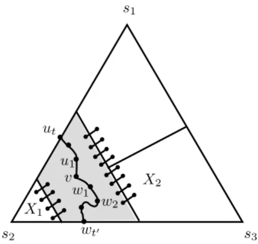
Let G = (∆3,n, E3,n) where E3,n := {xy : x, y ∈ ∆3,n,kx− yk1 = 2/n}. Their instance is obtained by dividing ∆3,n into a middle hexagon H := {x ∈ ∆3,n : xi ≤ 2/3 ∀i∈[3]} and three corner trianglesT1, T2, T3, where Ti :={x∈∆3,n :xi >2/3}.
To define the edge costs, we let ρ:= 3/(5n). The cost of the edges in G[H] isρ. The cost of the non-boundary edges inG[Ti] that are not parallel to the opposite side ofei is alsoρ. The cost of the non-boundary edges inG[Ti] that are parallel to the opposite side of ei are zero. The cost of the boundary edges in Lij are as follows: the edge closest toei has cost (n/3)ρ, the second closest edge to ei has cost (n/3−1)ρ, and so on. See Figure 2 for an example. We will denote the resulting graph with edge-costs asJ. The cost of a subsetF of edges on the instance J is CostJ(F) :=P
e∈Fw(e).
For a subset of edges F ⊂ E3,n, let G −F denote the graph (∆3,n, E3,n \F). We need the following two results about their instance. The first result shows that the cost of non-opposite cuts on their instance is at least 1.2.
Lemma 6.1. [1] For every non-opposite cutQ: ∆3,n →[4], the cost ofQon instance J is at least 1.2−n1.
The second result shows that if we remove a set of edges to ensure that a terminal si cannot reach any node in the opposite side Vjk, then the cost of such a subset of edges is at least 0.4.
Lemma 6.2. For {i, j, k}= [3] and for every subset F of edges in E3,n such that si cannot reach Vjk in G −F, the cost ofF on instance J is at least 0.4−(1n)/3.
6.1 The gap instance in [1] 16
s2 s3
s1 3̺
3̺
3̺
3̺
3̺
3̺
2̺
̺
2̺ ̺ ̺ ̺ ̺ ̺ 2̺
2̺
̺
̺
̺
̺
̺ 2̺
2̺
̺
̺
̺
̺
Figure 2: The instance in [1] for n= 9.
Although Lemma 6.2 is not explicitly stated in [1], its proof appears under Case 1 in the Proof of Lemma 3 of [1]. The factor 0.4 that we have here is because we scaled their costs by a factor of 6/5.
We next define non-oppositeness as a property of the cut-set as it will be convenient to work with this property for cut-sets rather than for cuts.
Definition 6.3. A set F ⊆E3,n of edges is a non-opposite cut-set if there is no path froms1 toV23 in G −F, no path from s2 toV13 inG −F, and no path froms3 to V12 inG −F.
We summarize the connection between non-opposite cut-sets and non-opposite cuts.
Proposition 6.4.
(i) If Q: ∆3,n →[4]is a non-opposite cut, then δ(Q) is a non-opposite cut-set.
(ii) For every non-opposite cut-set F ⊆E3,n, the cost of F on instance J is at least 1.2− 1n.
Proof. (i) Suppose not. Without loss of generality, suppose there exists a path from s1 toV23inG −δ(Q). Then, by the definition of δ(Q), all nodes of the path have the same label, so there exists a nodeu∈V23 that is labeled as 1, contradicting the fact that Qis a non-opposite cut.
(ii) Consider a labeling L : ∆3,n → [4] whereL =i if the nodev is reachable from terminal si in G −F and L(v) = 4 if the node v is reachable from none of the three terminals inG −F. Since F is a non-opposite cut-set, it follows that` is a non-opposite cut. Moreover,δ(L)⊆F. Therefore, the claim follows by Lemma 6.1.
6.2 Proof of Lemma 4.5 17
6.2 Proof of Lemma 4.5
We now restate and prove Lemma 4.5, i.e., a non-fragmenting non-opposite cut in
∆3,n that has lot of nodes labeled as 4 has large cost.
Lemma 6.5. Let Q : ∆3,n → [4] be a non-opposite cut with αn2 nodes labeled as 4. If Q is a non-fragmenting cut and n ≥ 10, then the cost of Q on J is at least 1.2 + 0.4α−n1.
Proof. We first show that the labeling Q may be assumed to indicate reachability in the graph G −δ(Q).
Claim 6.6. For every non-opposite non-fragmenting cut Q: ∆3,n →[4], there exists a labeling Q0 : ∆3,n →[4]such that
(i) a node v ∈∆3,n is reachable from si in G −δ(Q0) iff Q0(v) =i, (ii) CostJ(δ(Q0))≤CostJ(δ(Q)),
(iii) the number of nodes in ∆3,n that are labeled as 4 byQ is at most the number of nodes in ∆3,n that are labeled as 4 byQ0, and
(iv) Q0 is a non-opposite non-fragmenting cut.
s1
s2 s3 s2 s3
s1
1
2 4
1
3
2
3 1
4
Figure 3: An example of a cut Qand the cut Q0 obtained in the proof of Claim 6.6.
Proof. Fori∈[3], letSi be the set of nodes that can be reached from si in G −δ(Q).
Consider a labelingQ0 defined by Q0(v) :=
(i if v ∈Si, and
4 if v ∈∆3,n\(S1∪S2∪S3).
See Figure 3 for an example of a cut Q and the cut Q0 obtained as above. We prove the required properties for the labelingQ0 below.
(i) By definition, Q0(v) = iiff v is reachable from si in G \δ(Q0).
6.2 Proof of Lemma 4.5 18
(ii) Since δ(Q0) = (δ(S1)∪δ(S2)∪δ(S3))∩δ(Q), we have that δ(Q0)⊆δ(Q). Hence, CostJ(δ(Q0))≤CostJ(δ(Q)).
(iii) Let i ∈ [3]. Since all nodes of Si are labeled as i by Q, the nodes labeled as i byQ0 is a subset of the set of nodes labeled as i by Q. This implies that Q0 is also a non-opposite cut and that the number of nodes in ∆3,n that are labeled as 4 byQ is at most the number of nodes in ∆3,n that are labeled as 4 by Q0. (iv) SinceQis a non-fragmenting cut, there exist distincti, j ∈[3] such that|δ(Q)∩
Lij| = 1. Since δ(Q0) ⊆ δ(Q), we have that |δ(Q0)∩Lij| ≤ 1. On the other hand,Q0 labelssi byi and sj byj and hence, |δ(Q0)∩Lij| ≥1. Combining the two, we have that|δ(Q0)∩Lij|= 1 and hence Q0 is a non-fragmenting cut.
LetG0 :=G −δ(Q). By Claim 6.6, we may henceforth assume that
For every node v ∈V,v is reachable from si in G0 iff Q(v) = i. (1) In order to show a lower bound on the cost of Q, we will modify Q to obtain a non- opposite cut while reducing its cost by at least 0.4α. [1] showed that the cost of every non-opposite cut on J is at least 1.2− n1. Therefore, the cost of Q onJ must be at least 1.2− n1 + 0.4α.
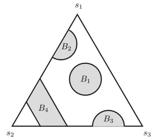
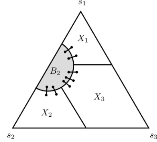
Since Q is a non-fragmenting cut, there exist distinct i, j ∈ [3] such that |δ(Q)∩ Lij| = 1. Without loss of generality, suppose that i = 1 and j = 3. For i ∈ [3], let Si := {v ∈ ∆3,n | Q(v) = i}, i.e. Si is the set of nodes that can be reached from si in G0. Let B :={v ∈ ∆3,n | Q(v) = 4} be the set of nodes labeled as 4 by Q. Then,
|B| =αn2. We note that S1, S2, and S3 are components of G0, and the set B is the union of the remaining components.
We recall that Vij is the set of end nodes of edges in Lij. We say that a node v ∈∆3,n can reachVij in G0 if there exists a path fromv to some node w∈Vij in G0. We observe that all nodes inV13are reachable from eithers1 ors3 inG0. In particular, this means that no node ofB can reach V13 inG0. We partition the node set B based on reachability as follows (see Figure 4):
B1 :={v ∈B | v cannot reach V12 and V23 in G0}, B2 :={v ∈B | v can reach V12 but not V23 in G0}, B3 :={v ∈B | v can reach V23 but not V12 in G0}, and B4 :={v ∈B |v can reach V12 and V23 in G0}.
Forr ∈[4], letβr :=|Br|/n2. We next summarize the properties of the sets defined above.
Proposition 6.7. The sets B1, B2, B3, B4 defined above satisfy the following proper- ties:
(i) For every distinct r, p∈[4], we have Br∩Bp =∅.
6.2 Proof of Lemma 4.5 19
s1
s2 s3
B4
B1
B2
B3
Figure 4: Partition of B into B1, B2, B3, B4.
(ii) For everyr ∈[4], we haveδ(Br)⊆δ(Q), i.e.Bris the union of some components of G0.
(iii) For every r ∈[4] and every edge e ∈δ(Br), one end node of e is in Br and the other one is in S1 ∪S2∪S3.
(iv) For every distinct r, p∈[4], we have δ(Br)∩δ(Bp) = ∅.
(v) B =∪4r=1Br,P4
r=1βr =α, and βr ≤0.66 for every r∈[4].
Proof. (i) The disjointness property follows from the definition of the sets.
(ii) Supposeδ(Br) is not a subset ofδ(Q) for somer ∈[4]. Without loss of generality, let r = 1 (the proof is similar for the other cases). Then, there exists an edge uv ∈ E3,n \δ(Q) with u∈ B1, v ∈ B\B1. Since v is in B\B1, it follows that the node v can reach either V12 or V13 in G0. Moreover, since the edge uv is in G0, it follows that the node u can also reach either V12 or V13 in G0, and hence u6∈B1. This contradicts the assumption that u∈B1.
(iii) Let uv ∈ δ(Br) with u ∈ Br and v 6∈ Br. Since Q(u) = 4, the node u is not reachable from any of the terminals in G0. Suppose that the node v is also not reachable from any of the terminals inG0. Then, by the reachability assumption, it follows that Q(v) = 4. Hence, the edge uv has both end-nodes labeled as 4 by Q and therefore uv 6∈ δ(Q). Thus, we have an edge uv ∈ δ(Bi) \δ(Q) contradicting part (ii).
(iv) Follows from parts (i) and (iii).
(v) By definition, we have that B = ∪4r=1Br. Since the sets B1, B2, B3, B4 are pair-wise disjoint, they induce a partition of B and hence |B| = P4
r=1|Br|.
Consequently, P4
r=1βrn2 = αn2 and thus, P4
r=1βr = α. Next, we note that
|∆3,n|= (n+ 1)(n+ 2)/2. Since Br ⊆B ⊆∆3,n, we have that βr =|Br|/n2 ≤
|∆3,n|/n2 ≤(1 + 1/n)(1 + 2/n)/2≤0.66 since n≥10.
6.2 Proof of Lemma 4.5 20
By Proposition 6.4 (i), the cut-set δ(Q) is a non-opposite cut-set. The following claim shows a way to modify δ(Q) to obtain a non-opposite cut-set with strictly smaller cost if βr>0.
Claim 6.8. For every r∈[4], there exists Er ⊆δ(Br), Er0 ⊆ G[Br] such that 1. Er⊆δ(Si) for somei∈[3],
2. (δ(Q)\Er)∪Er0 is a non-opposite cut-set and 3. CostJ(Er)−CostJ(Er0)≥0.4βr.
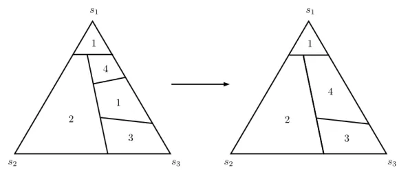
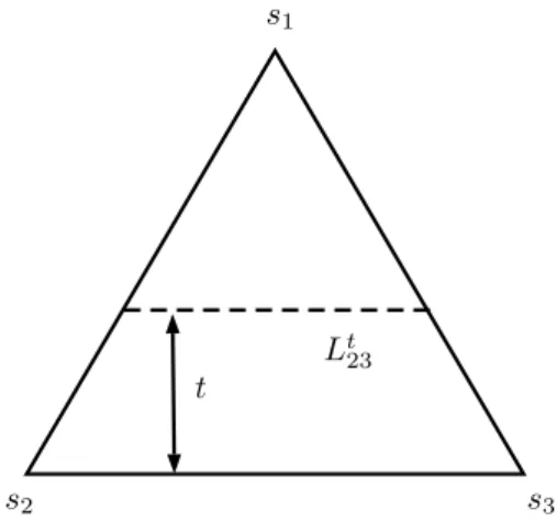
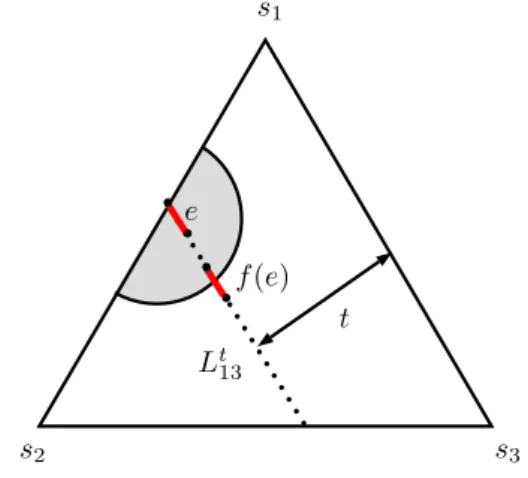
Proof. We consider the cases r = 1,2,4 individually as the proofs are different for each of them. The case of r = 3 is similar to the case of r = 2. We begin with a few notations that will be used in the proof. For distinct i, j ∈ [3], and for t ∈ {0,1, . . . ,2n/3}, let Vijt :={u∈∆3,n :uk = 1−t/nfor {k}= [3]\ {i, j}}. Thus, Vijt denotes the set of nodes that are on the line parallel toVij and at distance t/n from it. We will call the sets Vijt as lines for convenience. Let Ltij denote the edges of E3,n whose end-nodes are in Vijt. Thus, the edges in Ltij are parallel to Lij (see Figure 5).
s3
s2
s1
Lt23 t
Figure 5: The set of edges Lt23.
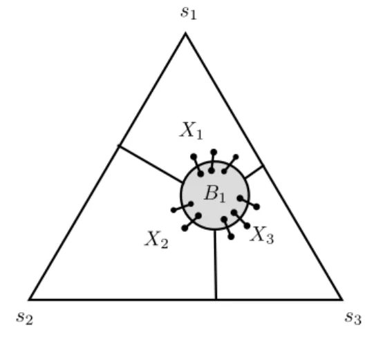
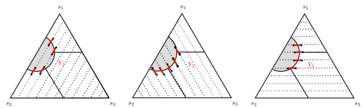
1. Suppose r = 1. We partition the set δ(B1) of edges into three sets Xi :=δ(B1)∩ δ(Si) for i∈[3] (see Figure 6).
By Proposition 6.7 (iii), we have that (X1, X2, X3) is a partition of B1. Let E1 := arg max{CostJ(F) :F ∈ {X1, X2, X3}} and
E10 :=∅.
We now show the required properties for this choice of E1 and E10.
(a) Since E10 = ∅, we need to show that δ(Q)\E1 is a non-opposite cut-set. Let G00:=G −(δ(Q)\E1). For each edge e∈E1, the end node ofe in ∆3,n\B1 is reachable from a terminalsi in G0 iff it is reachable fromsi in G00. Therefore, for each node v ∈ ∆3,n \B1 and a terminal si for i ∈ [3], we have that v is
![Figure 2: The instance in [1] for n = 9.](https://thumb-eu.123doks.com/thumbv2/9dokorg/775044.35049/17.892.303.599.148.421/figure-instance-n.webp)