Egerv´ ary Research Group
on Combinatorial Optimization
Technical reportS
TR-2017-09. Published by the Egerv´ary Research Group, P´azm´any P. s´et´any 1/C, H–1117, Budapest, Hungary. Web site: www.cs.elte.hu/egres. ISSN 1587–4451.
Beating the 2-approximation factor for Global Bicut
Krist´ of B´erczi, Karthekeyan Chandrasekaran, Tam´ as Kir´ aly, Euiwoong Lee, and Chao Xu
October 2017
EGRES Technical Report No. 2017-09 1
Beating the 2-approximation factor for Global Bicut
Krist´ of B´ erczi
?, Karthekeyan Chandrasekaran
??, Tam´ as Kir´ aly
?, Euiwoong Lee
? ? ?, and Chao Xu
??Abstract
In the fixed-terminal bicut problem, the input is a directed graph with two specified nodes and the goal is to find a smallest subset of edges whose removal ensures that the two specified nodes cannot reach each other. In the global bicut problem, the input is a directed graph and the goal is to find a smallest subset of edges whose removal ensures thatthere exist two nodes that cannot reach each other. Fixed-terminal bicut and global bicut are natural extensions of{s, t}-min cut and global min-cut respectively, from undirected graphs to directed graphs.
Fixed-terminal bicut is NP-hard, admits a simple 2-approximation, and does not admit a (2−)-approximation for any constant >0 assuming the unique games conjecture. In this work, we show that global bicut admits a (2−1/448)- approximation, thus improving on the approximability of the global variant in comparison to the fixed-terminal variant.
1 Introduction
The global minimum cut problem is a classic interdiction problem that admits efficient algorithms in undirected graphs. In this work, we study the following generalization of the global minimum cut problem from undirected graphs to directed graphs:
BiCut: Given a directed graph, find a smallest subset of edges whose removal ensures that there exist two distinct nodes that cannot reach each other.
A natural approach to solvingBiCutis by iterating over all pairs of distinct nodes s and t in the input graph and solving the following fixed-terminal bicut problem:
{s, t}-BiCut: Given a directed graph with two specified terminal nodes s, t, find a smallest subset of edges whose removal ensures thats and t cannot reach each other.
?MTA-ELTE Egerv´ary Research Group, Department of Operations Research, E¨otv¨os Lor´and University, Budapest, Email: {berkri,tkiraly}@cs.elte.hu. Krist´of and Tam´as are supported by the Hungarian National Research, Development and Innovation Office – NKFIH grants K109240 and K120254 and by the ´UNKP-17-4 New National Excellence Program of the Ministry of Human Capacities.
??University of Illinois, Urbana-Champaign. Email: {karthe,chaoxu3}@illinois.edu. Chao is supported in part by NSF grant CCF-1526799.
? ? ?Carnegie Mellon University, Pittsburgh. Email: euiwoonl@cs.cmu.edu
1.1 Results 2
Clearly, {s, t}-BiCut is equivalent to 2-terminal multiway-cut in directed graphs (the goal ink-terminal multiway cut is to remove a smallest subset of edges to ensure that the givenkterminals cannot reach each other). A classic result by Garg, Vazirani and Yannakakis shows that {s, t}-BiCut is NP-hard [9]. A simple 2-approximation algorithm is to return the union of a minimum s→ t cut and a minimum t →s cut in the input directed graph. The approximability of {s, t}-BiCut has seen renewed interest in the last few months culminating in inapproximability results matching the best-known approximability factor [4, 15]: {s, t}-BiCut has no efficient (2−)- approximation for any constant > 0 assuming the Unique Games Conjecture [14].
These results suggest that we have a very good understanding of the complexity and the approximability of the fixed-terminal variant, i.e.,{s, t}-BiCut. In contrast, even the complexity of the global variant, i.e., BiCut, is still an open problem.
The motivations for studyingBiCutare multifold. In many network defense/attack applications, global cuts and connectivity are much more important than connectivity between fixed pairs of terminals. On the one hand,BiCutis a fundamental global cut problem with interdiction applications involving directed graphs. On the other hand, there is no known complexity theoretic result forBiCut. The fundamental nature of the problem coupled with the lack of basic tractability results are compelling reasons to investigate this problem.
Furthermore, BiCut is an ideal candidate problem to study towards understand- ing whether cut problems exhibit a dichotomous behaviour between global and fixed- terminal variants in directed graphs. For concreteness, we recall the 3-Cut problem and the 3-way-Cut problem in undirected graphs. In 3-Cut, the input is an undi- rected graph and the goal is to find a smallest subset of edges whose removal ensures that there exist 3 nodes that cannot reach each other. In 3-way-Cut, the input is an undirected graph with 3 specified nodes and the goal is to find a smallest subset of edges whose removal ensures that the 3 specified nodes cannot reach each other.
While the global variant, namely 3-Cut, admits an efficient algorithm [10, 13], the fixed-terminal variant, namely 3-way-Cut, is NP-hard [7]. Such a dichotomy in complexity/approximability between global and fixed-terminal variants is hardly un- derstood in directed graphs. In this work, we exhibit such a dichotomy for directed graphs by focusing on BiCut.
1.1 Results
In spite of an extensive body of literature on cut problems in directed graphs, the complexity of BiCut is still an open problem. In this work, we exhibit a dichotomy in the approximability between BiCut and {s, t}-BiCut. While {s, t}-BiCut is inapproximable to a constant factor better than 2 assuming UGC, we show thatBi- Cutis approximable to a constant factor that is strictly better than 2. The following is our main result:
Theorem 1.1. There exists an efficient (2−1/448)-approximation algorithm for Bi- Cut.
We emphasize that the complexity of BiCutis still an open problem.
1.1 Results 3
Additional Results on Sub-problems. As a sub-problem in the algorithm for Theorem 1.1, we consider the following problem:
(s,∗, t)-Lin-3-Cut (abbreviating linear 3-cut): Given a directed graph D = (V, E) and two specified nodes s, t ∈ V, find a smallest subset of edges to remove so that there exists a node r with the property that s cannot reach r and t, and r cannot reach t in the resulting graph.
(s,∗, t)-Lin-3-Cut is a global variant of (s, r, t)-Lin-3-Cut, introduced in [8], where the input specifies three terminals s, r, t and the goal is to find a smallest subset of edges whose removal achieves the property above. A simple reduction from 3-way-Cut shows that (s, r, t)-Lin-3-Cut is NP-hard. The approximability of (s, r, t)-Lin-3-Cut was studied by Chekuri and Madan [4]. They showed that the inapproximability factor coincides with the flow-cut gap of an associated path- blocking linear program assuming the Unique Games Conjecture. However, the exact approximability factor is still unknown. On the positive side, there exists a simple combinatorial 2-approximation algorithm for (s, r, t)-Lin-3-Cut.
A 2-approximation for (s,∗, t)-Lin-3-Cut can be obtained by iterating over all choices for the terminalrand using the above-mentioned 2-approximation for (s, r, t)- Lin-3-Cut. However, for the purposes of getting a strictly better than 2-approxima- tion for BiCut, we need a strictly better than 2-approximation for (s,∗, t)-Lin-3- Cut. We obtain the following improved approximation factor:
Theorem 1.2. There exists an efficient 3/2-approximation algorithm for (s,∗, t)- Lin-3-Cut.
We emphasize that, similar to BiCut, we do not know if (s,∗, t)-Lin-3-Cut is NP-hard. Upon encountering cut problems in directed graphs whose complexity is difficult to determine, it is often insightful to consider the complexity of the analogous problem in undirected graphs. Our next result shows that the undirected counterpart of (s,∗, t)-Lin-3-Cut is in fact solvable in polynomial time. We observe that reach- ability in undirected graphs is a symmetric property: if a node s can reach another node t, then the node t can also reach the node s. Hence, the analogous problem in undirected graphs is the following: given an undirected graph with two specified nodess, t, remove a smallest subset of edges so that the resulting graph has at least 3 connected components with s and t being in different components. More generally, we consider the following:
{s, t}-Sep-k-Cut: Given an undirected graph G = (V, E) with two specified nodes s, t∈ V, find a smallest subset of edges to remove so that the resulting graph has at least k connected components with s and t being in different components.
The complexity of {s, t}-Sep-k-Cut for constant k was posed as an open problem by Queyranne [17]. In this work, we resolve this open problem by showing that {s, t}-Sep-k-Cut is solvable in polynomial-time for every constant k.
Theorem 1.3. For every constant k, there is an efficient algorithm to solve {s, t}- Sep-k-Cut.
1.2 Related Work 4
Organization. We set the notation and discuss another cut problem which is useful as a subproblem in our algorithm in Section 1.3. We prove Theorems 1.2 and 1.3 in Section 2 and Theorem 1.1 in Section 3.
A preliminary version of this work, together with related hardness results, appeared in the Proceedings of APPROX 2017 [2].
1.2 Related Work
In spite of an extensive literature on cut problems, we are unaware of any work on BiCut. We mention some work related to the other two problems mentioned in the previous section. (s, r, t)-Lin-3-Cutwas introduced by Erbacher et al. in [8]. They showed that the problem is fixed-parameter tractable when parameterized by the size of the solution.
k-Cut is a well-known partitioning problem in undirected graphs with a rich his- tory. In k-Cut, the input is an undirected graph and the goal is to find a smallest subset of edges to remove so that the resulting graph has at leastk connected compo- nents. Whenkis part of the input, this is NP-hard [10] and admits a 2-approximation [18]. When k is a constant, this is solvable in polynomial time [10, 13, 20].
The fixed-terminal variant of k-Cut is known as k-Way-Cut. In k-Way-Cut, the input is an undirected graph with k specified terminals s1, . . . , sk and the goal is to find a smallest subset of edges to remove so that no two terminals can reach each other in the resulting graph. It is well-known that k-Way-Cut is NP-hard [7]. For k = 3, a 12/11-approximation is known [5, 11], while for constant k, the current-best approximation factor is 1.2975 due to Sharma and Vondr´ak [19]. These results are based on an LP-relaxation proposed by C˘alinescu, Karloff and Rabani [6], known as the CKR relaxation. Manokaran, Naor, Raghavendra and Shwartz [16]
showed that the inapproximability factor coincides with the integrality gap of the CKR relaxation. Recently, Angelidakis, Makarychev and Manurangsi [1] exhibited instances with integrality gap at least 6/(5 + (1/k−1))− for everyk ≥3 and every >0 for the CKR relaxation.
1.3 Preliminaries
We recall another cut problem in digraphs that is used as a subproblem in our algo- rithm. Given a directed graph D = (V, E), we call a node to be a source if it can reach every other node inD. The following subproblem is used in our algorithm:
DoubleCut: Given a directed graph, find a smallest subset of edges to remove so that the resulting graph has no source node.
DoubleCut is also an extension of global minimum cut from undirected graphs to directed graphs. The tractability of DoubleCut is folklore (e.g., see [3]). We will need the specific structure of an optimal solution to DoubleCut. The following characterization of directed graphs with no source node shows the needed structure:
Theorem 1.4. (E.g., see [3]) Let D= (V, E) be a directed graph. The following are equivalent:
Section 2.Lin3Cutproblems 5
1. D has no source node.
2. There exist two disjoint non-empty setsS, T ⊂V with δin(S)∪δin(T) =∅.
From the above theorem, we conclude that every optimal solution to Double- Cutis given by the incoming edges of two disjoint non-empty subsets of nodes. The efficient algorithms for solvingDoubleCutcan be used to obtain such a pair of sets.
Notations. LetD = (V, E) be a directed graph. For two disjoint setsX, Y ⊂V, we denote δD(X, Y) to be the set of edges (u, v) with u ∈X and v ∈ Y and d(X, Y) to be the cut value |δD(X, Y)|. We useδDin(X) :=δD(V \X, X),δoutD (X) :=δ(X, V \X), dinD(X) := |δinD(X)| and doutD (X) := |δout(X)|. We drop the subscripts when the graph Dis clear from context. We use a similar notation for undirected graphs by dropping the superscripts in and out. For two nodes s, t ∈ V, a subset X ⊂ V is an st-set if t∈X ⊆V −s. The cut value of anst-set X is din(X). For two sets A, B ⊆V, let
β(A, B) := |δin(A)∪δin(B)|, and σ(A, B) := |δin(A)|+|δin(B)|.
2 Lin3Cut problems
In this section, we prove Theorems 1.2 and 1.3. Theorem 1.2 gives a 3/2-approxima- tion for (s,∗, t)-Lin-3-Cut and is a necessary component of our proof of Theorem 1.1. Theorem 1.3 is an investigation of (s,∗, t)-Lin-3-Cut in undirected graphs and answers an open problem posed by Queyranne [17].
2.1 A 3/2-approximation for (s, ∗, t)-Lin-3-Cut
One of our main tools used in the approximation algorithm for BiCut is a 3/2- approximation algorithm for (s,∗, t)-Lin-3-Cut. We present this algorithm now. We recall the problem (s,∗, t)-Lin-3-Cut: Given a directed graph with specified nodes s, t, find a smallest subset of edges whose removal ensures that the graph contains a noder with the property that s cannot reachr and t, and r cannot reach t.
Notations. LetV be the node set of a graph. A familyC of subsets ofV is achain if for every pair of setsA, B ∈ C, we have A⊂B orB ⊂A. We observe that a chain family can have at most |V| non-empty sets. Two sets A and B are uncomparable if A\B and B\A are non-empty. A setA is compatible with a chain C if C ∪ {A} is a chain, and it isnot compatible otherwise.
We first rephrase the problem in a convenient way.
Lemma 2.1. (s,∗, t)-Lin-3-Cut in a directed graph D= (V, E) is equivalent to min{β(A, B) :t∈A(B ⊆V − {s}}.
2.1 A 3/2-approximation for (s,∗, t)-Lin-3-Cut 6
Proof. LetF ⊆E be an optimal solution for (s,∗, t)-Lin-3-Cutin D and let (A, B) := argmin{β(A, B) :t∈A(B ⊆V −s}.
Let us fix an arbitrary node r∈ B−A. Since the deletion of δin(A)∪δin(B) results in a graph with no directed path froms tor, fromr totand from stot, the edge set δin(A)∪δin(B) is a feasible solution to (s, r, t)-Lin-3-Cutin D, thus implying that
|F| ≤β(A, B).
On the other hand, F is a feasible solution for (s, r0, t)-Lin-3-Cut in D for some r0 ∈V − {s, t}. LetA0 be the set of nodes that can reach tinD−F, andR0 be the set of nodes that can reachr0 inD−F. Then,F ⊇δin(A0). Moreover, F ⊇δin(R0∪A0) sinceR0∪A0 has in-degree 0 inD−F, andsis not inR0∪A0 because it cannot reachr0 and tin D−F. Therefore, taking B0 =R0∪A0 we getF ⊇δin(A0)∪δin(B0).
The above reformulation shows that the optimal solution is given by a chain consist- ing of twost-sets. The following lemma shows that we can obtain a 3/2 approximation to the required chain.
Lemma 2.2. There exists an efficient algorithm that given a directed graph D = (V, E) with nodes s, t ∈V returns a pair of st-sets A(B ⊆V such that
β(A, B)≤ 3
2min{β(A, B) :t ∈A(B ⊆V − {s}}.
Proof. The objective is to find a chain of two st-sets A, B with minimum β(A, B).
To obtain an approximation, we build a chain C ofst-sets with the property that, for some valuek ∈Z+,
(i) every set C ∈ C is a st-set with din(C)≤k, and (ii) every st-set T with din(T) strictly less than k is in C.
We use the following procedure to obtain such a chain: We initialize with k being the minimum st-cut value and C consisting of a single minimum st-cut. In a general step, we find twost-sets: a st-setY compatible with the current chain C, i.e. C ∪ {Y} forming a chain, with minimumdin(Y) and ast-setZ not compatible with the current chain C, i.e. crossing at least one member of C, with minimum din(Z). We will later see that such setsY andZ can be found in polynomial time. Ifdin(Y)≤din(Z), then we add Y toC, and set k todin(Y); otherwise we set k to din(Z), and stop.
Proposition 2.3. Let C denote the chain before any general step of the above-men- tioned procedure. Then, for every C ∈ C and for every st-set A that is not in C, we have
din(A)≥din(C).
Proof. Let A be a st-set that is not in C. Suppose for the sake of contradiction that din(A) < din(C) for some C ∈ C. Let C0 denote the chain consisting of those members of C that were added before C. Since A 6∈ C and C is a set of minimum cut value compatible withC0, we have thatA should cross at least one member of C0. Hence, by din(A) < din(C), the procedure stops before adding C to the chain C0, a contradiction.
2.1 A 3/2-approximation for (s,∗, t)-Lin-3-Cut 7
Proposition 2.4. The chain C and the value k obtained at the end of the above- mentioned procedure satisfy (i) and (ii).
Proof. The construction immediately guarantees that every set C ∈ C is a st-set. By Proposition 2.3 and by construction of C and k, we have that din(C) ≤ k for every C ∈ C and hence, we have (i).
By construction,C contains allst-setsT that are compatible withC withdin(T)< k.
Suppose for the sake of contradiction, we have anst-set T withdin(T)< k that is not in C. Then, the set T should be incompatible with C. We note that the procedure terminates by setting k = din(Z) for some Z that is incompatible with C. However, the setT is a contradiction to the choice ofZ in the procedure. Therefore, there does not exist ast-set T with din(T)< k that is not in C and hence, we have (ii).
By the above, the procedure stops with a chainC containing allst-sets of cut value less thank, and anst-setZ of cut value exactlykwhich crosses some memberX ofC.
If the optimum value of our problem is less thank, then both members of the optimal pair (A, B) belong to the chain C, and we can find them by taking the minimum of β(A0, B0) where A0 ⊂B0 with A0, B0 ∈ C.
We can thus assume that the optimum is at leastk. Since din(Z) =k anddin(X)≤ k, the submodularity of the in-degree function implies
din(X∩Z) +din(X∪Z)≤din(Z) +din(X)≤2k.
Hence either din(X∩Z)≤k ordin(X∪Z)≤k. Since
d(X\Z, X ∩Z) +d(Z\X, X ∩Z)≤din(X∩Z) and d(V \(X∪Z), X \Z) +d(V \(X∪Z), Z \X)≤din(X∪Z), at least one of the following four possibilities holds:
1. din(X∩Z)≤k and d(X\Z, X∩Z)≤ 12k. Choose A=X∩Z, B =X. Then β(A, B) =d(X\Z, X∩Z) +din(X)≤ 12k+k= 32k.
2. din(X∩Z)≤k and d(Z \X, X ∩Z)≤ 12k. Choose A=X∩Z, B =Z. Then β(A, B) =d(Z\X, X ∩Z) +din(Z)≤ 12k+k = 32k.
3. din(X ∪Z)≤ k and d(V \(X∪Z), X \Z)≤ 12k. Choose A =Z, B =X∪Z.
Then β(A, B) =din(Z) +d(V \(X∪Z), X \Z)≤k+12k = 32k.
4. din(X∪Z)≤k and d(V \(X∪Z), Z\X)≤ 12k. Choose A =X, B =X∪Z.
Then β(A, B) =din(X) +d(V \(X∪Z), Z\X)≤k+12k = 32k.
Thus a pair (A, B) can be obtained by taking the minimum among the four possi- bilities above andβ(A0, B0) whereA0 ⊂B0 withA0, B0 ∈ C, concluding the proof of the approximation factor. It remains to ensure that the algorithm can be implemented to run in polynomial-time.
The algorithm is summarized below. Step 2(a) to obtainY can be implemented to run in polynomial-time as follows: lett∈C1 ⊂. . . ,⊂Cq ⊆V −sdenote the members
2.2 An exact algorithm for {s, t}-Sep-k-Cut 8
of C. Find a minimum cut Yi with Ci ⊆Yi ⊆V \Ci+1 for i= 1, . . . , q, and choose Y to be a minimum one among these cuts. Step 2(b) to obtain Z can be implemented to run in polynomial-time as follows: for each pairx, y of nodes with y∈Ci ⊆V −x for some i∈ {1, . . . , q}, find a minimum cut Zxy with {t, x} ⊆Zxy ⊆V − {s, y}, and choose Z to be a minimum one among these cuts. Since C is a chain, we have that q≤ |V|and hence both steps can be implemented to run in polynomial-time.
Approximation Algorithm for (s,∗, t)-Lin-3-Cut Input: Directed graphD= (V, E) with s, t∈V
1. Let S denote the sink-side of a minimum s → t cut and α denote its value.
InitializeC ← {S}and k ←α.
2. Repeat:
(a) Y ←arg min{din(Y) :Y is a st-set compatible with C}
(b) Z ←arg min{din(Z) :Z is a st-set not compatible with C}
(c) If din(Y)≤din(Z), then update C ← C ∪ {Y} and k ←din(Y).
(d) Else, update k ←din(Z), set X to be a set inC that crosses Z and go to Step 3.
3. Let (A, B)←arg min{β(A, B) :A, B ∈ C, A6=B}.
4. Let (S, T)←arg min{β(X∩Z, X), β(X∩Z, Z), β(Z, X∪Z), β(X, X ∪Z)}
5. Return arg min{β(A, B), β(S, T)}.
Theorem 1.2 is a consequence of Lemmas 2.1 and 2.2. The approximation algorithm is summarized below.
2.2 An exact algorithm for {s, t}-Sep-k-Cut
In this section, we show that {s, t}-Sep-k-Cut is solvable in polynomial time if k is a fixed constant. We recall the problem {s, t}-Sep-k-Cut: Given an undirected graph with specified nodes s, t, find a smallest subset of edges whose removal ensures that the resulting graph has at least k connected components with s and t being in different components.
Notations. Let G = (V, E) be an undirected graph. Let the minimum size of an {s, t}-cut in G be denoted by λG(s, t). For two subsets of nodes X, Y, we recall that d(X, Y) denotes the number of edges betweenX andY and thatd(X) = d(X, V \X).
The cut value of a partition {V1, . . . , Vq} of V is defined to be the total number of
2.2 An exact algorithm for {s, t}-Sep-k-Cut 9
crossing edges, that is, (1/2)Pq
i=1d(Vi), and is denoted by γ(V1, . . . , Vq). Let γq(G) denote the value of an optimum q-Cut inG, i.e.,
γq(G) := min{γ(V1, . . . , Vq) :Vi 6=∅ ∀ i∈[q],
Vi∩Vj =∅ ∀ i, j ∈[q],∪qi=1Vi =V}.
Proof of Theorem 1.3. Letγ∗ denote the optimum value of {s, t}-Sep-k-Cut inG= (V, E) and let H denote the graph obtained from G by adding an edge of infinite capacity between s and t. The algorithm is based on the following observation (we recommend the reader to considerk = 3 for ease of understanding):
Proposition 2.5. Let {V1, . . . , Vk} be a partition of V corresponding to an optimal solution of {s, t}-Sep-k-Cut, where s is in Vk−1 and t is in Vk. Then we have γ(V1, . . . , Vk−2, Vk−1∪Vk)≤2γk−1(H).
Proof. Let W1, . . . , Wk−1 be a minimum (k −1)-cut in H. Clearly, s and t are in the same part, so we may assume that they are in Wk−1. Let U1, U2 be a minimum {s, t}-cut in G[Wk−1]. Then {W1, . . . , Wk−2, U1, U2} gives an {s, t}-separating k-cut, showing that
γ∗ ≤γ(W1, . . . , Wk−2, U1, U2) =γk−1(H) +λG[Wk−1](s, t). (1) By Menger’s theorem, we have λG(s, t) pairwise edge-disjoint paths P1, . . . , PλG(s,t) betweens and t inG. Consider one of these paths, sayPi. If all nodes of Pi are from Vk−1∪Vk, then Pi has to use at least one edge from δ(Vk−1, Vk). Otherwise,Pi uses at least two edges fromδ(V1∪ · · · ∪Vk−2)∪ [
i,j≤k−2 i6=j
δ(Vi, Vj). Hence the maximum number of pairwise edge-disjoint paths betweens and t is
λG(s, t)≤d(Vk−1, Vk) + 1 2
d(V1∪ · · · ∪Vk−2) + X
i,j≤k−2 i6=j
d(Vi, Vj)
.
Thus, we have
γ∗ =d(Vk−1, Vk) +d(V1∪ · · · ∪Vk−2) + X
i,j≤k−2 i6=j
d(Vi, Vj)
≥λG(s, t) + 1 2
d(V1∪ · · · ∪Vk−2) + X
i,j≤k−2 i6=j
d(Vi, Vj)
=λG(s, t) + 1
2γ(V1, . . . , Vk−2, Vk−1∪Vk)
≥λG[Wk−1](s, t) + 1
2γ(V1, . . . , Vk−2, Vk−1∪Vk)
Section 3.BiCut 10
that is,
γ∗ ≥λG[Wk−1](s, t) + 1
2γ(V1, . . . , Vk−2, Vk−1∪Vk). (2) By combining (1) and (2), we get γ(V1, . . . , Vk−2, Vk−1∪Vk)≤2γk−1(H), proving the proposition.
Karger and Stein [13] showed that the number of feasible solutions to k-Cut in an undirected graph Gwith value at most 2γk(G) isO(n4k). All these solutions can be enumerated in polynomial-time for fixed k [12, 13, 21]. This observation together with Proposition 2.5 gives the algorithm for finding an optimal solution to {s, t}- SepEdgekCut. The algorithm is summarized below.
Algorithm for {s, t}-Sep-k-Cut
Input: Undirected graph G= (V, E) with s, t∈V
1. Let H be the graph obtained from G by adding an edge of infinite ca- pacity between s and t. In H, enumerate all feasible solutions to Edge- (k −1)-Cut—namely the vertex partitions {W1, . . . , Wk−1}—whose cut value γH(W1, . . . , Wk−1) is at most 2γk−1(H). Without loss of generality, assume s, t∈Wk−1.
2. For each feasible solution to Edge-(k −1)-Cut in H listed in Step 1, find a minimum{s, t}-cut inG[Wk−1], say U1, U2.
3. Among all feasible solutions {W1, . . . , Wk−1} to Edge-(k − 1)-Cut listed in Step 1 and the corresponding U1, U2 found in Step 2, return the k-cut {W1, . . . , Wk−2, U1, U2} with minimumγ(W1, . . . , Wk−2, U1, U2).
The correctness of the algorithm follows from Proposition 2.5: one of the choices enumerated in Step 1 will correspond to the partition (V1, . . . , Vk−2, Vk−1∪Vk), where (V1, . . . , Vk) is the partition corresponding to the optimal solution.
3 BiCut
In this section, we present our approximation algorithm (Theorem 1.1) for BiCut. We begin with the high-level ideas of the approximation algorithm in Section 3.1. The full algorithm and the proof of its approximation ratio are presented in Section 3.2.
We recall the problem BiCut: Given a directed graph, find a smallest number of edges in whose removal ensures that there exist two distinct nodes s and t such that scannot reacht and t cannot reachs. We begin with a reformulation of BiCutthat is helpful for the purposes of designing an algorithm. We recall that for two sets of nodesA, B, the quantity β(A, B) =|δin(A)∪δin(B)|.
3.1 Overview of the Approximation Algorithm 11
Definition 3.1. We define two sets A and B to be uncomparable if A\B 6=∅ and B\A6=∅. For a directed graph D= (V, E), let
β := min{β(A, B) : A and B are uncomparable}.
The following lemma shows that bicut is equivalent to finding an uncomparable pair of subsets of nodes A, B with minimum β(A, B).
Lemma 3.2. BiCut in a given directed graph D= (V, E) is equal to β.
Proof. IfA andB are uncomparable and we removeδin(A)∪δin(B) from the directed graph, then nodes in A\B cannot reach nodes inB\A and vice versa. On the other hand, ifs cannot reacht and t cannot reachs, then the set of nodes that can reach s and the set of nodes that can reacht are uncomparable, and have in-degree 0.
Using the above formulation, and by recalling that σ(A, B) = |δin(A)|+|δin(B)|, we have the following natural relaxation of bicut:
Definition 3.3. For a directed graph D= (V, E), let
σ := min{σ(A, B) : A and B are uncomparable}.
A pair where the latter value is attained is called a minimum uncomparable cut-pair.
3.1 Overview of the Approximation Algorithm
In this section, we sketch the argument for a (2−)-approximation for some small enough. We observe that for every pair of subsets of nodes (A, B), we have
β(A, B) = σ(A, B)−d(V \(A∪B), A∩B). (3) Therefore, β(A, B) ≤ σ(A, B) ≤ 2β(A, B) for every pair of subsets of nodes (A, B) and henceβ ≤σ ≤2β. Furthermore,σ can be computed efficiently (see Lemma 3.4).
Hence, we immediately have a (2−)-approximation if σ ≤ (2−)β. On the other hand, ifσ >(2−)β, thend(V \(A∪B), A∩B)>(1−)β for every minimizer (A, B) of β(A, B), thus providing a structural handle on optimal solutions. Our algorithm proceeds by making several attempts at finding pairs (A0, B0) that could give a (2−)- approximation. Each attempt that is unsuccessful at giving a (2−)-approximation implies some structural property of the optimal solution. These structural properties are together exploited by the last attempt to succeed.
Our next attempt is to solve a constrained variant of BiCut: For fixed Z ⊆ V, we would like to find an uncomparable pair (A, B) satisfying A∩B = Z that minimizesβ(A, B) among pairs with this property. This problem is solvable efficiently by reducing toDoubleCut (see Lemma 3.5). The same holds when V \(A∪B) is fixed. In particular, if there is a pair (A, B) that minimizes β(A, B) and|A∩B| ≤2 or|V \(A∪B)| ≤2, then we can find the minimizer efficiently. Therefore we assume that every minimizer (A, B) forβ(A, B) satisfies |A∩B| ≥ 3 and |V \(A∪B)| ≥ 3.
Let us fix one such minimizer (A, B).
3.1 Overview of the Approximation Algorithm 12
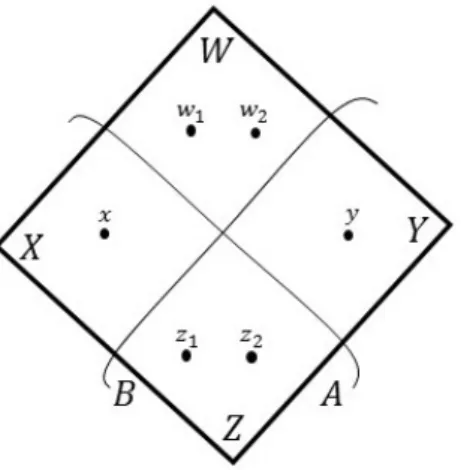
In the algorithm, we guess nodes x ∈ A\B, y ∈ B \A, w1, w2 ∈ V \(A∪B), and z1, z2 ∈ A∩B. The reason for guessing two nodes as opposed to just one node in the intersection and in the complement of the union is highly technical (it certifies a detailed structural property of the minimizer (A, B)), and is not relevant to this overview. We use the notation X := A\B, Y := B \A, W := V \(A∪B), and Z :=A∩B (see Figure 1).
Figure 1: The partitioning of the node set in the graph D. Here, (A, B) denotes the optimum bicut that is fixed.
We now observe that A is the sink-side of a {w1, w2, y} → {x, z1, z2}-cut while B is the sink-side of a {w1, w2, x} → {y, z1, z2}-cut. Our next attempt in the algorithm is to find (X0, Y0), where X0 is the sink-side of a minimum {w1, w2, y} → {x, z1, z2}- cut, and Y0 is the sink-side of the minimum {w1, w2, x} → {y, z1, z2}-cut. The hope behind this attempt is that X0 could be A and Y0 could be B as these are feasible solutions to the respective problems and thus, they would together help us recover the optimal solution. Unfortunately, this favorable best-case scenario may not happen.
Yet, owing to the feasibility ofA andB for the respective problems, we may conclude that σ(X0, Y0)≤σ(A, B)≤2β(A, B) = 2β.
Our subsequent attempts are more complex and proceed by refiningX0 andY0. For our next attempt, we observe that Z is the sink-side of a {w1, w2, x, y} → {z1, z2}- cut. So, our next attempt in the algorithm would be to find Z0 as the sink-side of a minimum {w1, w2, x, y} → {z1, z2}-cut and expand X0 and Y0 by Z0 to obtain an uncomparable pair (A0 =X0∪Z0, B0 =Y0∪Z0). Our hope is to find a Z0 so that the resulting β(A0, B0) is small. While finding Z0, we prefer not to have many edges of E[X0]∪E[Y0] in the new bicut (A0, B0). This is because, such edges enter only one among the two setsA0 andB0. We recall that if we have an uncomparable pair (A0, B0) with lot of edges fromV \(A0∪B0) to A0∩B0, then the value of β(A0, B0) is going to be much less than σ(A0, B0) (e.g., see (3)), thus leading to a (2−)-approximation.
So, in order to avoid the edges of E[X0]∪E[Y0] in the new bicut (A0, B0), we make such edges more expensive by duplicating them before finding Z0. Let D1 be the digraph obtained by duplicating the edges in E[X0]∪E[Y0], and let Z0 be the sink- side of the minimum{w1, w2, x, y} → {z1, z2}-cut inD1. We then show that the pair
3.1 Overview of the Approximation Algorithm 13
(X0∪Z0, Y0∪Z0) is a (2−)-approximation unless|δDin1(Z)|>(2−3)β, thus giving us more structural handle on the optimum solution.
We next make an analogous attempt by shrinkingX0 andY0 instead of expanding.
LetD2be the digraph obtained by duplicating the edges inE[V\X0]∪E[V\Y0], and let W0 be the source-side of the minimum {w1, w2} → {x, y, z1, z2}-cut in D2. We obtain that the pair (X0\W0, Y0\W0) is a (2−)-approximation unless|δDout2(W)|>(2−3)β.
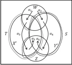
Figure 2: The quantities α1, . . . , α6.
Letα1, . . . , α6 be the number of edges in each position indicated in Figure 2. If the attempts so far are unsuccessful, then we use the structural properties derived so far to arrive at the following:
1. All but O(β) edges inδin(X0)∪δin(Y0)∪δout(W)∪δin(Z) are as positioned in Figure 2.
2. The quantities α1, α3, α5 are within O(β) of each other (see (29), (30), (31)) and so are α2, α4, α6.
3. Furthermore, (1−O())β =α3+α4 ≤β (see Proposition 3.12).
Without loss of generality, we may assume α3 ≥ α4. Hence, by conclusion (3) from above, we have that α3 ≥β/2−O()β.
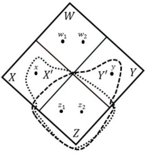
Our final attempt in the algorithm to obtain a (2− )-approximate bicut is to expandY0 by including some nodes fromX0\Y0 and to shrinkX0 by excluding some nodes from X0\Y0. We now explain the motivation behind this choice of expanding and shrinking. Consider S :=Y0 ∪(X0 ∩Z), which is obtained by expanding Y0 by including some nodes from X0\Y0 and T :=X0\(X0∩(W \Y0)), which is obtained by shrinking X0 by excluding some nodes from X0 \Y0 (see figure 3). By definition, (S, T) is an uncomparable pair. We will now see that the bicut value of (S, T) is much
3.1 Overview of the Approximation Algorithm 14
smaller than 2β. Using conclusions (1) and (2) from above, we obtain that β(S, T) =|δin(Y0∪(X0∩Z))∪δin(X0\(X0∩(W \Y0)))|
=|δin(Y0)| −α5+α3+|δin(X0)| −α1+O()β (4)
=σ(X0, Y0)−α1−α5+α3+O()β (5)
≤2β−α3+O()β (6)
≤ 3
2β+O()β. (7)
In the above, equation (4) is by using conclusion (1), equation (5) is by definition of σ, inequality (6) is by using conclusion (2) and σ(X0, Y0) ≤ σ(A, B) ≤ 2β, and inequality (7) is becauseα3 ≥β/2−O()β.
Figure 3: The motivation behind the last attempt.
Although (S, T) is a good approximation to the optimal bicut, we cannot obtain the setsS and T without the knowledge of W and Z (which, in turn, depend on the optimal bicut (A, B)). Instead, our algorithmic attempt is to expand Y0 by including some nodes fromX0\Y0 and to shrinkX0 by excluding some nodes from X0\Y0. In other words, our candidate is a pair (B0, Y0 ∪A0) for some X0 ∩Y0 ⊆ A0 ( B0 ⊆ X0 (we need the condition A0 ( B0 because B0 and Y0 ∪A0 should be uncomparable).
When choosingA0 and B0, we ignore the edges whose contribution do not depend on A0 and B0. Let H be the digraph obtained by removing the edges inE[Y0∪(V \X0)].
Our aim is to minimize |δHin(B0)∪δHin(Y0∪A0)|. However, this quantity differs from
|δinH(A0)∪δinH(B0)| byO(β), so we may instead aim to minimize the latter.
The crucial observation now is that this latter minimization problem is an instance of (s,∗, t)-Lin-3-Cut. While we do not know how to solve (s,∗, t)-Lin-3-Cutopti- mally, we can efficiently obtain a 3/2-approximation by Theorem 1.2. By the refor- mulation of (s,∗, t)-Lin-3-Cut in Lemma 2.1, we get a pair of subsets (A0, B0) for which X0 ∩Y0 ⊆ A0 ( B0 ⊆ X0 and which is a 3/2-approximation. In particular,
3.2 Approximation Algorithm and Analysis 15
|δinH(A0)∪δHin(B0)| ≤(3/2)|δHin((X0∩(Z∪Y0))∪δHin(X0\(W\Y0))| ≤3(α3+O()β)/2.
Using this and proceeding similar to the calculations shown above to obtain the bound on β(S, T) (i.e., 4, 5, 6, and 7), we derive that β(B0, Y0∪A0)≤ (7/4 +O())β, con- cluding the proof.
3.2 Approximation Algorithm and Analysis
In this section we prove Theorem 1.1 by giving an efficient (2−)-approximation algorithm for BiCut for a constant > 0. We will describe the algorithm, analyze its approximation factor to show that it is (2−) for some constant and compute the value of at the end of the analysis.
We begin by showing that certain relaxations of β can be solved. We first show that σ can be computed efficiently.
Lemma 3.4. For a directed graph D = (V, E), there exists a polynomial time algo- rithm to find a minimum uncomparable cut-pair.
Proof. For fixed verticesa and b, there is an efficient algorithm to find A and B such thata∈A\B andb ∈B\Aandσ(A, B) is minimized. Indeed, this is precisely finding the sink side of a mina→b cut and that of a minb →acut. Trying all distinct pairs of nodes a and b and taking the minimum gives the desired result.
We next show that we can minimize β(A, B) among uncomparable pairs (A, B) whose intersection is fixed.
Lemma 3.5. Given a directed graphD= (V, E)andZ ⊆V, there exists a polynomial time algorithm to find an uncomparable pairA, B satisfyingA∩B =Z that minimizes β(A, B) among pairs with this property.
Proof. Let D0 = D[V \Z] be the directed graph induced on V \Z. We recall that DoubleCutcan be solved in polynomial time inD0 [3]; letX0 andY0 be the disjoint sets whose incoming edges give the optimal double cut. We claim that the pair X0∪Z, Y0∪Z forms a minimum bicut among all bicuts with intersection Z. Indeed, assume the optimal solution is β(A, B). Let X = A\ B, Y = B \A and W = V −(A∪B). Then
β(X0∪Z, Y0∪Z) = dinD0(X0) +dinD0(Y0) +din(Z)
≤dinD0(X) +dinD0(Y) +din(Z)
=din(Z) +d(W, X) +d(W, Y) +d(X, Y) +d(Y, X)
=β(A, B).
A similar argument shows that we can minimizeβ(A, B) among uncomparable pairs (A, B) for which the complement of the union is fixed.
3.2 Approximation Algorithm and Analysis 16
Lemma 3.6. Given a directed graph D = (V, E) and W ⊆V, there exists a polyno- mial time algorithm to find an uncomparable pair A, B satisfying V \(A∪B) = W that minimizes β(A, B) among pairs with this property.
We need the following definition.
Definition 3.7. If c is a capacity function on a directed graph D, then dinc (U) = P
e∈δin(U)c(e) is the sum of the capacities of incoming edges ofU. Similarly,doutc (U) = P
e∈δout(U)c(e).
We now present the approximation algorithm and the analysis.
Proof of Theorem 1.1. The algorithm is summarized below. We first note that the algorithm indeed returns the bicut value of an uncomparable pair. The run-time of the algorithm being polynomial follows from Lemmas 2.2, 3.4, 3.5 and 3.6. In the rest of the proof, we analyze the approximation factor. We will show that the algorithm achieves a (2−)-approximation factor and compute at the end.
Approximation Algorithm for BiCut Input: Directed graphD= (V, E)
1. Compute (S, T)←arg min{σ(S, T) :S and T are uncomparable}using Lemma 3.4 and setµ1 ←β(S, T)
2. Compute µ2 ←min{β(A, B) :A and B are uncomparable, |A∩B| ≤2} using Lemma 3.5
3. Compute µ3 ← min{β(A, B) : A and B are uncomparable, |V \(A∪B)| ≤ 2}
using Lemma 3.6 4. Initialize µ4 ← ∞
5. For each tuple of nodes (x, y, z1, z2, w1, w2)
(i) X0 ← sink-side of the minimum {w1, w2, y} → {x, z1, z2}-cut (ii) Y0 ← sink-side of the minimum {w1, w2, x} → {y, z1, z2}-cut (iii) E1 ←E[X0]∪E[Y0]
(iv) E2 ←E[V \X0]∪E[V \Y0]
(v) D1 ← Dwith the arcs in E1 duplicated (vi) D2 ← Dwith the arcs in E2 duplicated
(vii) Z0 ←sink-side of minimum {w1, w2, x, y} → {z1, z2}-cut in D1 (viii) W0 ← source-side of minimum {w1, w2} → {x, y, z1, z2}-cut inD2
(ix) H ← contract X0∩Y0 toz0, contract V \X0 tow0, remove all w0z0 arcs (x) In H, find w0z0-sets A0 (B0 such that β(A0, B0) is at most
(3/2) min{β(A, B) :z0 ∈A(B ⊂V − {w0}}using Lemma 2.2
3.2 Approximation Algorithm and Analysis 17
(xi) A1 ←(A0\ {z0})∪(X0∩Y0) and B1 ←(B0\ {z0})∪(X0 ∩Y0)
(xii) Find all bicuts that can be generated using set operations on X0, Y0, Z0, W0, A1, B1 and letµ04 denote the minimum bicut value among these.
(xiii) If µ04 < µ4, updateµ4 ←µ04 6. Return µ←min{µ1, µ2, µ3, µ4}.
To analyze the approximation factor, let us fix a minimizer (A, B) forBiCutin the input graph D= (V, E), i.e. fix an uncomparable pair (A, B) such thatβ(A, B) = β.
LetX :=A\B,Y :=B\A,Z :=A∩B, andW :=V \(A∪B) (see Figure 1). With this notation, we have
β =d(W∪Y, X) +d(W∪X, Y) +din(Z) =d(Y, X∪Z) +d(X, Y ∪Z) +dout(W). (8) We may assume that both Z and W are of size at least 3, otherwise the algorithm finds the optimum since it returns a value µ≤µ2, µ3. Let >0 be a constant whose value will be determined later.
Lemma 3.8. If one of the following is true, then σ ≤(2−)β:
(i) d(W, Z)≤(1−)β,
(ii) For every z1, z2 ∈ Z, there exists a subset U of nodes containing z1, z2 but not Z with din(U)<(1−)β.
(iii) For every w1, w2 ∈ W, there exists a subset U of nodes not containing w1, w2 but intersecting W with din(U)<(1−)β.
Proof.
(i) If d(W, Z) ≤ (1− )β, then σ(A, B) = β(A, B) +d(W, Z) ≤ (2− )β. The pair (A, B) is uncomparable, and hence σ ≤σ(A, B). Therefore, we have µ1 = β(S, T)≤σ(S, T) = σ≤σ(A, B)≤(2−)β.
(ii) Suppose condition (ii) holds. Among the sets with in-degree less than (1−)β which do not contain every node of Z, let T be the one with inclusionwise maximal intersection with Z. Such a set T exists since condition (ii) holds. Let z1 ∈ Z \T and z2 ∈ Z ∩T. There exists a set U containing z1, z2 but not Z with din(U)<(1−)β and z1, z2 ∈U. Because of the maximal intersection ofT with Z, we have that T 6⊂U. Hence T and U are uncomparable and therefore σ ≤ σ(T, U) ≤ (2−2)β. Therefore, we have µ1 = β(S, T) ≤ σ(S, T) = σ ≤ σ(A, B)≤(2−2)β.
(iii) Argument similar to the proof of (ii) shows that the minimum uncomparable cut-pair is a (2−2)-approximation if condition (iii) holds.
3.2 Approximation Algorithm and Analysis 18
For the rest of the proof, we may assume that
σ≥(2−)β (9)
since otherwise, the algorithm returns µ ≤ µ1 = σ ≤ (2−)β. By Lemma 3.8, we have
d(W, Z)≥(1−)β. (10)
We also have verticesz1, z2 ∈Z and w1, w2 ∈W violating conditions(ii) and (iii) of Lemma 3.8 respectively. Let us fix such vertices, i.e.,
(a) fix z1, z2 ∈Z such that din(U)≥(1−)β for all subsets U of nodes containing z1, z2 but notZ, and
(b) fix w1, w2 ∈ W such that din(U) ≥ (1− )β for all subsets U of nodes not containingw1, w2 but intersectingW.
Also let us fix an arbitrary choice ofx∈X, y ∈Y (since Aand B are uncomparable, we have that X and Y are non-empty and hence such an x and y can be chosen).
Henceforth, we will consider the iteration of Step 5 in the algorithm for this choice of x, y, z1, z2, w1, w2.
We note that (X0, Y0) form an uncomparable pair. If β(X0, Y0) ≤ (2−)β, then the algorithm returns µ≤µ4 ≤(2−)β. Therefore, we may assume that
β(X0, Y0)≥(2−)β. (11) Also, we havedin(X0)≤din(X∪Z) becauseX0 is the sink-side of a min{w1, w2, y} → {x, z1, z2} cut. Since din(X∪Z)≤din(A)≤β, we have that
din(X0)≤β. (12)
Similarly,
din(Y0)≤din(Y ∪Z)≤β. (13) Consequently,
σ(X0, Y0)≤din(X0) +din(Y0)≤2β. (14) We consider four cases depending on the relations between W and X0 ∪Y0, and between Z and X0∩Y0.
Case 0. SupposeW∩(X0∪Y0) =∅,Z ⊆X0∩Y0 (see figure 4). In this caseδin(X0) andδin(Y0) both contain all edges counted ind(W, Z). Henceβ(X0, Y0)≤σ(X0, Y0)−
d(W, Z) ≤ (1 +)β. The second inequality here is because σ(X0, Y0) ≤ 2β by (14) and d(W, Z)≥(1−)β by 10. This shows that (X0, Y0) is a (1 +)-approximation.
Letc be the capacity function obtained by increasing the capacity of each edge in E1 to 2, and let ¯cbe the capacity function obtained by increasing the capacity of each edge inE2 to 2. For the remaining three cases, we will use the following proposition.
Proposition 3.9. If din(X0 ∩Z0) ≥ (1−)β and din(Y0 ∩Z0) ≥ (1−)β, then β(X0 ∪Z0, Y0∪Z0)≤2β+dinc (Z).
3.2 Approximation Algorithm and Analysis 19
Figure 4: The case where W ∩(X0∪Y0) = ∅,Z ⊆X0∩Y0. Proof. Ifdin(X0∩Z0)≥(1−)β, thendin(X0)−din(X0∩Z0)≤β. So
din(X0∪Z0) = din(Z0) +din(X0)−din(X0∩Z0)
−d(X0\Z0, Z0 \X0)−d(Z0\X0, X0\Z0) (15)
≤din(Z0) +β−d(X0\Z0, Z0 \X0)−d(Z0\X0, X0\Z0).
Hence, we have
din(X0∪Z0)≤din(Z0) +β−d(X0 \Z0, Z0\X0). (16) Similarly,
din(Y0 ∪Z0)≤din(Z0) +β−d(Y0 \Z0, Z0\Y0). (17) We need the following proposition.
Proposition 3.10.
β(X0∪Z0, Y0∪Z0)≤σ(X0∪Z0, Y0∪Z0) +dinc (Z0)−2din(Z0)
+d(X0\Z0, Z0\X0) +d(Y0\Z0, Z0\Y0). (18) Proof. By counting the edges entering Z0, we have
1. dinc (Z0) =din(Z0) +|δin(Z0)∩E1|.
2. din(Z0) =d(V \(X0∪Y0∪Z0), Z0) +|δin(Z0)∩E1|+d(X0\Z0, Z0\X0) +d(Y0\ Z0, Z0 \Y0)−d((X0∩Y0)\Z0, Z0\(X0∪Y0)).
The first equation can be rewritten as
dinc (Z0)−2din(Z0) =−din(Z0) +|δin(Z0)∩E1|.
Using this and the second equation, we get
dinc (Z0)−2din(Z0) +d(X0\Z0, Z0\X0) +d(Y0\Z0, Z0 \Y0)
=−d(V \(X0∪Y0∪Z0), Z0) +d((X0∩Y0)\Z0, Z0\(X0∪Y0)).
3.2 Approximation Algorithm and Analysis 20
Thus the desired inequality (18) simplifies to
β(X0∪Z0, Y0 ∪Z0)≤σ(X0∪Z0, Y0∪Z0)−d(V \(X0∪Y0∪Z0), Z0) +d((X0∩Y0)\Z0, Z0\(X0∪Y0)).
To prove this inequality, we observe that the edges counted by d(V \ (X0 ∪Y0 ∪ Z0), Z0) are counted twice in σ(X0∪Z0, Y0∪Z0). Hence we have the desired relation (18).
Using (18), (17) and (16) we get
β(X0∪Z0, Y0∪Z0)≤din(X0∪Z0) +din(Y0∪Z0) +dinc (Z0)−2din(Z0) +d(X0 \Z0, Z0\X0) +d(Y0\Z0, Z0\Y0)
≤din(Z0) +β+din(Z0) +β+dinc (Z0)−2din(Z0)
= 2β+dinc (Z0)
≤2β+dinc (Z).
The last inequality above is because Z is a feasible solution for the minimization problem that obtains Z0 and hencedinc (Z0)≤dinc (Z). This completes the proof of the proposition.
Case 1. Suppose W ∩(X0∪Y0) = ∅and Z 6⊆X0∩Y0. Without loss of generality, letZ 6⊆X0. The set X0∩Z0 containsz1, z2 but not the wholeZ, hencedin(X0∩Z0)≥ (1−)β by (a).
We first consider the subcase wheredin(Y0∩Z0)<(1−)β. By the choice ofz1, z2, this means that Z ⊆ Y0 ∩Z0. In this case Y0 ∩Z0 crosses X0, because X0 does not contain all vertices in Z, and Y0 ∩Z0 does not contain x. Thus (X0, Y0 ∩Z0) is an uncomparable pair. Now we observe that σ(X0, Y0∩Z0) = din(X0) +din(Y0 ∩Z0)≤ (2−)β. Thus, σ ≤(2−)β, a contradiction to (9).
Next we consider the other subcase where din(Y0 ∩Z0) ≥ (1 − )β. Then, by Proposition 3.9, we get
β(X0∪Z0, Y0 ∪Z0)≤2β+dinc (Z).
We are in the case where (X0∪Y0)∩W =∅, sodinc (Z)≤din(Z)+d(X, Z)+d(Y, Z). We now note thatdin(Z)+d(X, Z)+d(Y, Z) = 2din(Z)−d(W, Z)≤2β−(1−)β= (1+)β sinced(W, Z)≥(1−)βanddin(Z)≤β. Hence we haveβ(X0∪Z0, Y0∪Z0)≤(1+3)β.
Since (X0 ∪Z0, Y0∪Z0) is an uncomparable pair, we have that µ4 ≤(1 + 3)β.
Case 2. Suppose W∩(X0∪Y0)6=∅and Z ⊆X0∩Y0. This is similar to Case 1 by symmetry.