GERGELY AMBRUS, IMRE B ´AR ´ANY, P ´ETER FRANKL, D ´ANIEL VARGA
Abstract. We consider the minimum number of lineshnandpn needed to intersect or pierce, respectively, all the cells of the n×n chessboard. Determining these values can also be interpreted as a strengthening of the classical plank problem for integer points.
Using the symmetric plank theorem of K. Ball, we prove that hn=dn2efor each n≥1.
Studying the piercing problem, we show that 0.7n ≤pn ≤ n−1 for n ≥ 3, where the upper bound is conjectured to be sharp. The lower bound is proven by using the linear programming method, whose limitations are also demonstrated.
1. Cells and lines
How many lines are needed to pierce each cell of the n×nchessboard? Likewise, what is the minimum number of lines required to intersect every cell? These innocent-looking questions serve as targets of the present note.
The question of determining pn was raised by B´ar´any and Frankl in [BF21,BF21+]. It turns out that the question has a close connection with the classical plank problem in the plane [B51, T32]. In particular, the celebrated symmetric plank theorem of K. Ball [B91]
implies that given any set ofn−1 lines, there always exists a point (x, y) in [0, n−1]2 such that the interior of the cell [x, x+ 1]×[y, y+ 1] is not intersected by any of the lines. The present question boils down to the following (see Conjecture 5): does there exist aninteger point with the same property? If true, this would provide a significant strengthening of the plank theorem in this special case, and could also initiate the study of plank problems for lattice points. Even though we are not able to give a complete answer to the above question, we show nontrivial bounds on pn (see Theorem 4).
To start with, we introduce some notations. Forn≥1, letQndenote then×nchessboard embedded in [−1,1]2. Itscells are the closed squares
(1) cij =
−1 + (i−1)· 2
n,−1 +i· 2 n
×
−1 + (j−1)· 2
n,−1 +j· 2 n
with i, j ∈[n], where [n] = {1, . . . , n}. A line`⊂R2 is said tohit orintersect a cellcij if
`∩cij 6=∅, and it pierces cij if `∩intcij 6= ∅. Let hn and pn be the minimal number of lines needed to hit or pierce, respectively, each cell of Qn.
Our first observations are trivial. Clearly,hn≤pnholds for eachn. Piercing each column of Qn with a vertical line shows that pn ≤ n. More generally, all the cells of Qn can be pierced bynparallel lines in any given direction which are at distance n2 from each other in the `1 distance and do not go through any grid points. On a similar note, selecting every second vertical boundary line between the cells of Qnyields that hn≤ dn2e.
It is easy to give a sharp upper bound for the number of cells pierced by an arbitrary line. The following simple statement is part of the mathematical folklore (see also [B83]):
Date: November 19, 2021.
2020Mathematics Subject Classification. Primary 11H31, secondary 05B40, 52C30.
Key words and phrases. Cells in a lattice, lines, discrete plank problems.
1
arXiv:2111.09702v1 [math.CO] 18 Nov 2021
Proposition 1. Every line pierces at most 2n−1 cells of Qn.
This readily implies that pn ≥ n2. We note that higher dimensional versions of this estimate have been recently studied by B´ar´any and Frankl [BF21,BF21+].
Note that the analogue of Proposition1does not hold for hitting: diagonals of the square Qnintersect 3ncells. Nevertheless, using the symmetric plank theorem of K. Ball, we prove that the upper bound on hngiven above is sharp:
Theorem 2. For each n≥1, hn=dn2e holds.
Determiningpnproves to be more difficult. Surprisingly, and somewhat counter-intuitively, the upper bound pn≤n can be improved: there exist several configurations of n−1 lines piercing all the cells of Qn. This is also the subject of a mathematics puzzle [BS19] that appeared in The Guardian.
Theorem 3. p2= 2 and for eachn≥3, pn≤n−1.
The lower bound pn ≥ n2 is not sharp either: using linear programming methods, we asymptotically strengthen it. Here comes our main result.
Theorem 4. If nis sufficiently large, then pn>0.7n.
The gap between the upper and lower estimates for pn is large, and there is certainly room for improvement. A computer search was carried out in order to find configurations ofn−2 lines piercing all cells ofQn whenn≤15, to no avail. Based on this computational evidence, we venture to formulate the following conjecture.
Conjecture 5. For all n≥3, pn=n−1.
Note that the Corollary of [B91] implies that given a set of n−1 lines, there always exists a translate of a cell contained within Qn which is not pierced by any of these lines.
Conjecture 5is the analogue of this statement for lattice cells.
Even though the linear programming method used for proving Theorem 3 may be strengthened, in Section 5 we demonstrate its limitations. Theorem 9 states that this method cannot give a lower bound larger than 0.925n. The proof Conjecture5will require novel ideas.
2. Hitting
In this section we prove Theorem 2. We use the symmetric plank theorem of K. Ball.
Lemma 6 (Ball [B91]). If (ϕi)m1 is a sequence of unit functionals in a finite-dimensional normed space X, (ti)m1 is a sequence of reals and (wi)m1 is a sequence of positive numbers with Pm
1 wi= 1 then there is a point in the unit ball of X for which
|ϕi(x)−ti| ≥wi
for every i∈[m].
Proof of Theorem 2. By the remark preceding Proposition 1 it suffices to prove hn≥ dn2e.
Assume on the contrary that there exists a set of m := dn2e −1 lines, {`1, . . . , `m}, inter- secting each cell of Qn. Let ui denote the (Euclidean) unit normal of `i. Let X be the space R2 endowed with the`∞-norm, that is, with unit ball [−1,1]2. To each planar vector u6= 0, assign the linear functional
(2) ϕu : x7→ hx, ui
kuk1
which has norm 1 in X∗. Setϕi:=ϕui for each i∈[m]. Then
(3) `i={x∈R2 : ϕi(x) =ti}
holds for every i ∈ [m] with some ti ∈ R. Note that the set of points x ∈ R2 for which
|ϕi(x)−ti| ≤ w holds equals to the union of all (closed) squares of edge length 2w whose center lies on `i.
Setε >0 so that (2n+ε)(dn2e −1) = 1, and let wi= n2 +εfor everyi. Lemma6implies the existence of x∈[−1,1]2 for which
|ϕi(x)−ti| ≥ 2 n+ε
holds for each i. This is equivalent to the fact that the open square x+
− 2 n−ε,2
n +ε2
is not met by any of the lines `i. We finally observe that any open square of side length strictly greater than n4 centered in [−1,1]2 contains a cell of Qn.
3. A piercing construction
To each line `we assign the corresponding “snake”σ(`) of cells ofQn which are pierced by `:
(4) σ(`) ={cij : i, j∈[n] and `pierces cij} (see the shaded region on Figure 1.a)).
We continue with a nontrivial upper bound on pn.
Proof of Theorem 3. We will construct a set of n−1 lines which pierces every cell of Qn. Define the line ` by the equation
y= (1−ε)x
where ε >0 is a small positive number, for instance ε= n12 will do. Thus, `is obtained by a small clockwise rotation of the line y=x about the origin, see Figure1a).
Let now
`i =`+
1−2i+ 1
n ,−1 +2i+ 1 n
for each i∈ [n−2], see Figure 1b). Then `i passes through the center of the cell c(n−i)i and intersects its boundary on its two vertical sides (because its slope is slightly less than one). Choose the value of ε so that σ(`i) contains exactly three cells in row i, at most 2 cells in any other row ofQn, and`i does not pass through any vertex of a cell inQn. Then along with any cell of σ(`i), it also contains a horizontal or vertical neighbour of the cell.
Since `i+1 is obtained from `i by a translation with (−2n,n2), this implies that Sn−2 i=1 σ(`i) covers each cell ofQnin between`1 and`n−2 (simply check the off-diagonal chains of cells).
Therefore, the lines `1, . . . , `n−2 pierce all the cells of Qn except c1n, c2n and c(n−1) 1cn1. Clearly these four cells can be pierced by one line `0, which leads to a set of n−1 lines
piercing every cell of Qn.
We note that the above construction is not unique. Indeed, the same pattern works using translates of a line which pierces exactly 3 consecutive cells in some row and does not pass through any grid point. Thus, for any α∈(13,1) there exists a set ofn−2 lines of slopeα, along with a line of slope −n−1n−2 which pierceQn.
Figure 1. Piercing Qn withn−1 lines.
Going even further, we challenge the dedicated reader to find a piercing configuration which consists of kparallel lines of an approximately diagonal direction andn−1−k lines in the orthogonal direction, for each k ∈ [n−2]. (The two families of lines have to be positioned in a cross-like pattern, so that every boundary cell is pierced by them.)
4. Few lines do not pierce
Proof of Proposition 1. Assume the slope of `is non-negative. We move a point on `from left to right and order the cells in σ(`) (cf. (4)) in the order the point enters them. If cij ∈σ(`), then the next cell in this order is either c(i+1)j orci(j+1). The cells in σ(`) thus
form a zig-zag going left or up at each step.
The lower boundpn≥ n2 follows from Proposition1. We are going to improve this lower bound by the linear programming method that yields the following statement. Below, x= (x, y), and dkxk1 stands for d(|x|+|y|).
Lemma 7. Assume thatµ: [−1,1]2→R≥0 is a Lipschitz continuous density function such that for each line `in the plane,
(5)
Z
`∩[−1,1]2
µ(x) dkxk1 ≤1.
Then for any ε >0,
pn>1 2
Z
[−1,1]2
µ(x) dx−ε n
holds if n is sufficiently large.
Proof. Denote by L the set of all lines intersecting [−1,1]2, and set Sn ={σ(`) : `∈ L}.
So Sn is the set of all snakes. Clearly, Sn is a finite set, and for every element ofSn there exists a line which pierces the cells therein. Determining pn is equivalent to finding the optimal value of the following integer linear program (LPi):
(LPi)
Minimize X
σ∈Sn
ρ(σ) subject to ρ(σ)∈ {0,1} for all σ∈ Sn, and
X
σ∈Sn:cij∈σ
ρ(σ)≥1 for every i, j∈[n].
Therefore, the optimal value of the following continuous linear program (LPc) gives a lower bound onpn:
(LPc)
Minimize X
σ∈Sn
ρ(σ) subject to ρ(σ)≥0 for all σ∈ Sn, and
X
σ∈Sn:cij∈σ
ρ(σ)≥1 for every i, j∈[n].
Taking the dual program of (LPc) leads to the following setup. Let w: [n]×[n]→[0,1]
be a weight function, and use the notation wij = w(i, j). Let M be the solution of the following continuous linear program:
(LPd)
Maximize
n
X
i,j=1
wij subject to wij ≥0 for every i, j= [n] and
X
i,j∈[n]:cij∈σ(`)
wij ≤1 for every line `.
By weak linear programming duality, the optimal valueM of (LPd) gives a lower bound on that of (LPc), which in turn gives a lower bound on the solution of (LPi). Thus,
(6) pn≥M.
(Note that this fact also follows elementarily, without referring to LP duality. The above linear programs depend on nbut we suppress this dependence.)
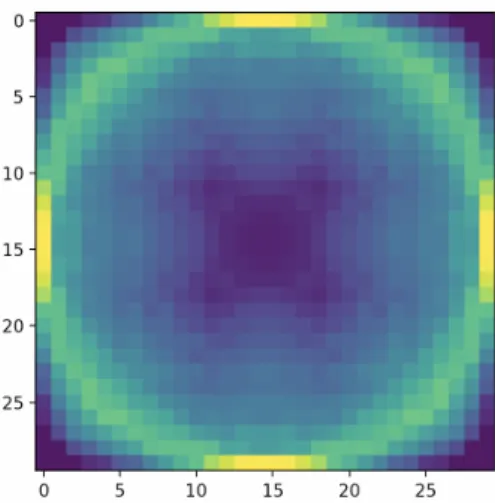
Thus, we face the problem: How to solve (LPd)? Since there are only finitely many snakes in Sn, the number of constraints in (LPd) is finite. Therefore, (LPd) can be solved computationally, at least for small values of n. In the case n = 30, the optimal weight distribution onQnfound by computational methods is plotted on Figure2. This yields the estimate pn≥0.7205nforn= 30.
However, for large values of n the computational approach brakes down; solving the n= 30 case already required several days of computing. We are going to replace (LPd) by its continuous approximation when n→ ∞.
Let µ: [−1,1]2 →R≥0 be a density function which is Lipschitz continuous with respect to the Euclidean distance, with constant λ. To each cell cij ofQn we assign the weight
(7) wij = n
2 Z
cij
µ(x) dx
where dxstands for the standard Lebesgue measure. Note that (8)
n
X
i,j=1
wij = n 2
Z
[−1,1]2
µ(x) dx.
On the other hand, for each line`defined by the equationϕu(x) =t(cf. (2)), we introduce the corresponding plank
(9) P(`) =n
x∈h
−1− 2 n,1 + 2
n i2
: |ϕu(x)−t| ≤ 1 n
o .
Figure 2. Optimal weight distribution on Qn with n= 30, where darker (blue) colors represent values close to 0.
ThenP(`) is the intersection of [−1−2n,1 +n2]2with the union of the squares of edge length
2
n centered on `. Note that P(`) is not contained inQn, a small part of it is outside.
Figure 3. Comparison of the regions P(`) and S(`)
Claim 8. Using the above notations, for each line`∈ L, X
i,j,∈[n]: cij∈σ(`)
wij ≤ n 2
Z
P(`)
µ(x) dx+34λ n .
Proof. We may assume that the slope of `is non-positive. Then, the upper boundary line of P(`) is obtained from the lower boundary line by a translation withv= (n2,n2).
Let
S(`) = [
σ(`)
cij.
Notice thatS(`)∩(S(`) +v) =∅andS(`)∩(S(`)−v) =∅. Observe that if a cellcij ∈σ(`) reaches below P(`), then (cij\P(`)) +v ⊂P(`), and similarly, if cij ∈σ(`) reaches above P(`), then (cij\P(`))−v⊂P(`), unlesscij is at the boundary ofQ0n(see Figure 3). Thus, the parts ofS(`) which are not contained inP(`) may be moved intoP(`) by a translation with eithervor−v, without creating overlaps (note that this is the reason for definingP(`)
on [−1−n2,1 +n2]2 instead of [−1,1]2). Therefore, by the Lipschitz property of µ, X
i,j,∈[n]:cij∈σ(`)
wij = n 2
Z
S(`)
µ(x) dx≤ n 2
Z
P(`)
µ(x) +2√ 2 n λ
! dx
≤ n 2
Z
P(`)
µ(x) dx+√
2λArea(P(`))
≤ n 2
Z
P(`)
µ(x) dx+
√ 2λ·2
n·4
1 + 2 n
≤ n 2
Z
P(`)
µ(x) dx+34λ
n .
Now, the proof of the Lemma is easy to complete. The Lipschitz property of µensures that as n→ ∞,
n 2
Z
P(`)
µ(x) dx+34λ
n →
Z
`∩[−1,1]2
µ(x) dkxk1.
Thus, (5) guarantees that the weights wij given by (7) satisfy the criterion of (LPd), and hence by (6) and (8), n2 R
[−1,1]2µ(x) dxprovides a lower bound on pn. In view of Lemma 7, the next task is to find a suitable density function on [−1,1]2. Proof of Theorem 4. In order to illustrate the method, we will first consider the following density function which leads to a slightly weaker estimate:
(10) µ1(x) = 3
4(x2−2x2y2+y2)
(see Figure4a). The functionµ1(x) is clearly Lipschitz. We will show that (5) holds forµ1. Assume that the line ` is defined by the equation y = ax+b. By the symmetries of µ(x), for proving (5) we may assume that a ∈ [0,1] and b ≥ 0. Also, if ` hits [−1,1]2, then b ≤ 1 +a must hold. Let x1 = (x1, y1) and x2 = (x2, y2), x1 ≤ x2 be the points where ` hits the boundary of [−1,1]2 (these may coincide when ` hits only a corner). By the assumptions on a and b, we have that x1 = −1 and y1 ∈ [−1,1]. Depending on the magnitude of b,x2 may lie on the upper or the right side of [−1,1]2:
• if 0≤b≤1−a, thenx2 = 1 and y2=a+b;
• if 1−a≤b≤1 +a, then x2 = 1−ba andy2 = 1.
Accordingly, (5) is equivalent to
(11) max
a∈[0,1],b∈[0,1−a](1 +a) Z 1
−1
(x2−2x2(ax+b)2+ (ax+b)2) dx≤ 4 3 and
(12) max
a∈[0,1],b∈[1−a,1+a](1 +a) Z 1−b
a
−1
(x2−2x2(ax+b)2+ (ax+b)2) dx≤ 4 3. By evaluating the above integrals, (11) reads as
a∈[0,1],b∈[0,1−a]max (1 +a) 2 3−2a2
15 +2b2 3
!
≤ 4 3.
It is simple to check that the above function attains its maximum on the given domain at a= 0, b= 1 with the maximum value being exactly 43. Similarly, (12) amounts to
a∈[0,1],b∈[1−a,1+a]max
(1 +a)(−1 + 5a2+ 5a3−a5+ 5b2+ 5a3b2−5b3−5a2b3+b5)
15a3 ≤ 4
3. By analyzing the function above, one obtains that for any given a ∈ [0,1], the above function is maximized at b= (−1−a+√
9−6a+ 9a2)/2 on the intervalb∈[1−a,1 +a].
Substituting this value leads to a function of awhich is decreasing on (0,1].
Thus, we obtain that the maximum ofR
`∩[−1,1]2µ1(x) dkxk1 is attained for lines`which contain a side of [−1,1]2, with the extreme value being 1. Since
Z
[−1,1]2
µ1(x) dx= 4 3, Lemma 7 guarantees that for anyε >0,
pn>
2 3−ε
n ifn is sufficiently large.
The stronger estimate pn>0.7nof Theorem 4can be shown by considering the density function
µ2(x) = 0.3(|x|+|y|) + 0.43(|x|3+|y|3)−0.585(|x|3|y|+|y|3|x|)−0.16x2y2
(see Figure 4b), which has been found by numerical optimization. Clearly, µ2 is Lipschitz on [−1,1]2, and
Z
[−1,1]2
µ2(x) dx≈1.4039.
That (5) is satisfied forµ2is again checked by elementary calculus, although the calculations are more tedious than in the previous case because of the absolute values in the definition of µ2(x). We only note that, using the notation above, the maximum line integral is taken at a = 0.5612, b = 0.5612 with the maximum value being approximately 0.9971. Thus, because of the symmetries taken into account, lines of maximal weight go close to a corner of [−1,1]2, and they are of slope around 0.56, −0.56, 1.78 or −1.78. Further calculations may be completed by the aid of a computer algebra software.
5. Limitations of the linear programming method
Along the lines of the previous section, one may increase the lower bound on pn by including higher order terms in the density function, although at the price of increased computational difficulty. However, in this section we prove that the conjectured value pn=n−1 can not be proved by applying the continuous linear programming method. In order to show that, note that any feasible solution of the linear program (LPc) yields an upper bound on the optimal value of (LPc), hence, by linear programming duality, on that of (LPd) as well. Therefore, in order to demonstrate the confinedness of the LP method, it suffices to provide a weight distribution ρ(σ) on the set S of snakes which satisfies the constraints of (LPc) and for which P
σ∈Sρ(σ) < n−1. We will, in fact, prove a much stronger bound.
(a) The functionµ1(x, y) (b) The functionµ2(x, y) Figure 4. The two density functions used in the proof of Theorem 4.
Darker (blue) colors represent values close to 0, while lighter (yellow) stands for values close to 0.75.
Theorem 9. For every sufficiently large n, there exists a weight distribution ρ(σ) on Sn satisfying the conditions of (LPc) for which
X
σ∈Sn
ρ(σ)<0.925n.
Recall that L is the set of lines intersecting [−1,1]2. We parameterize L as follows: for each s∈[−1,1], introduce the vector
us= (s,1− |s|) and for each s, t∈[−1,1], define
(13) `(s, t) ={x∈R2 : ϕus =t}
(cf. (2)). That is,`(s, t) is the line with normalus defined by sx+ (1− |s|)y =t. It is easy to check that `∈ L if and only if it may be expressed in the form (13) with s, t∈[−1,1].
Reminiscent of Lemma7, we will construct the sought-after weight distribution on S by applying a continuous approximation.
Lemma 10. Assume that ν : [−1,1]2 → R≥0 is a Lipschitz continuous density function which satisfies that for each (x0, y0)∈[−1,1]2,
(14)
Z 0
−1
ν(s, y0+s(x0+y0)) ds+ Z 1
0
ν(s, y0+s(x0−y0)) ds≥1.
Then for any ε >0, the optimal value of (LPc) is bounded from above by 1
2 Z
[−1,1]2
ν(s, t) dsdt+ε n
if n is sufficiently large.
Proof. To each snake σ∈ Sn, assign the weight
(15) ρ(σ) = n
2 Z
(s,t)∈[−1,1]2:σ(`(s,t))=σ
ν(s, t) dsdt.
Clearly,
(16) X
σ∈Sn
ρ(σ) = n 2
Z
[−1,1]2
ν(s, t) dsdt.
In order for the weights ρ(σ) to satisfy the conditions of (LPc), the following inequality must hold for all i, j∈[n]:
(17) n
2 Z
(s,t)∈[−1,1]2:cij∈σ(`(s,t))
ν(s, t) dsdt≥1.
The above integration goes over the set of parameters (s, t) whose corresponding lines pierce cij. This region can be determined as follows. Let (x0, y0) be the center ofcij. Recall that the side-length of cij equals to n2. First, assume thats≤0, equivalently, that the slope of
`(s, t) is non-positive. Then `(s, t) pierces cij if and only if it contains a point of the form (x0+a, y0−a) with|a|< n1. That is equivalent to the condition
|s(x0+y0)−t+y0|< 1 n.
Similarly, if s ≥0, then `(s, t) intersects cij iff it goes through a point of the form (x0 + b, y0+b) with|b|< 1n, which is equivalent to
|s(x0−y0)−t+y0|< 1 n.
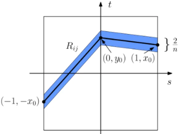
Thus, we derive that the set of lines in Lwhich piercecij is represented on the (s, t)-plane by the regionRij which is the vertical parallel neighborhood of radius n1 of the union of two segments, connecting the points (−1,−x0) and (0, y0), and (0, y0) and (1, x0), respectively.
In particular, all the cross-sections ofRij parallel to thet-axis are of length 2n(see Figure5).
Figure 5. The region Rij on the (s, t)-plane which represents the set of lines intersectingcij
By the Lipschitz property of ν, the integrals in (17) converge uniformly asn→ ∞:
n 2
Z
(s,t)∈[−1,1]2:cij∈σ(`(s,t))
ν(s, t) dsdt→ Z 0
−1
ν(s, y0+s(x0+y0)) ds+
Z 1
0
ν(s, y0+s(x0−y0)) ds.
Thus, (14) and (17) guarantee that the conditions of (LPc) hold for a suitably scaled copy of ρ provided by (15), and the statement of Lemma10 follows from (16).
We are left with the task of finding a suitable density function on the (s, t)-plane.
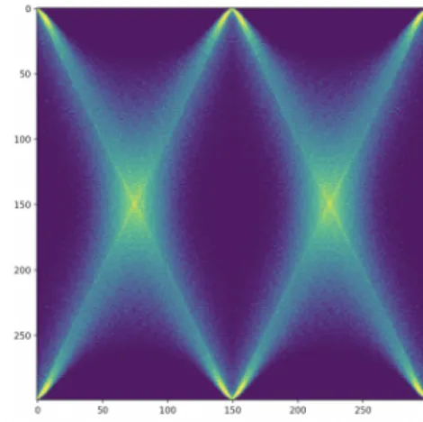
(a)Structure of the functionν(s, t) (b)Discrete density function on the 300×300 grid, found by computer search
Figure 6. Dual density functions on the (s, t)-plane
Proof of Theorem 9. We will construct a density function ν(s, t) which is not Lipschitz continuous, but satisfies (14) as well as
(18)
Z
[−1,1]2
ν(s, t) dsdt <1.849.
Lemma10 may then be applied to a suitably fine Lipschitz continuous approximation ofν, yielding the estimate of Theorem 9.
The density ν is defined using a parameter γ ∈[0,1] whose value we will set later. Let ε >0 be a small positive number. DefineP1 to be the parallelogram
P1= conv{(0,1),(−ε,1),(−1,−1),(−1 +ε,−1)}
of area 2ε. Let P2 ={(s, t) : (s,−t) ∈P1} be the mirror image of P1 with respect to the s-axis, and set P3 =−P1 and P4 =−P2. DefineP5 to be the rectangle
P5 = conv n
−1−ε 2 , h
,
−1 +ε 2 , h
,
−1 +ε 2 ,−h
,
−1−ε
2 ,−ho
where h = tan2γ +ε. Note that if ε <1− tan 12 , then h ∈[0,1). Finally, letP6 =−P5 (see Figure 6a).
We will say that a line `is ofangleα if its slope is tanα. Let π2 −β be the angle of the line connecting the points (−1 +ε/2,−1) and (−ε/2,1). Then tanβ = 1−ε2 .
Now, let ` be a line of angle α which goes through two points (−1, t1) and (0, t2) with t1, t2 ∈ [−1,1]. A simple calculation shows (see Figure 7a) that the horizontal projection of `∩P1 has length
εcosαcosβ cos(α+β) .
By symmetry, the horizontal projection of `∩P2 has length εcos(α−β)cosαcosβ. Let
(19) φ(α) = cosαcosβ
cos(α+β)+ εcosαcosβ cos(α−β) .
It is easy to check thatφ(α) is symmetric, convex on (−arctan 2,arctan 2), and it attains its minimum on this interval at 0 with φ(0) = 2. In particular,φ is increasing on [0,arctan 2].
(a) Scheme of`∩P1 (b) The case|α1|+|α2|< γ Figure 7
Next, we define the density function ν(s, t). Set w= 2φ(γ)1 . Denote byχAthe indicator function of the set A, and let
ν1(s, t) = w ε
4
X
i=1
χPi(s, t).
Introduce
ψ(t) =
1−φ(arctan 2t) φ(γ)
.
Then ψ(t) is convex on (−π2,π2) with the maximum value taken att= 0, and ψ(t) >0 for
|t| ≤h. Define
ν2(s, t) = (1
εψ(t) for (s, t)∈P5∪P6
0 otherwise,
and let ν(s, t) =ν1(s, t) +ν2(s, t). We will show thatν satisfies the condition (14).
Let x0, y0 ∈[−1,1] be arbitrary, and denote by α1 and α2 the angle of the lines through the points (−1,−x0) and (0, y0), and (0, y0) and (1, x0), respectively. Then, since φ is symmetric and convex,
Z 0
−1
ν1(s, y0+s(x0+y0)) ds+ Z 1
0
ν1(s, y0+s(x0−y0)) ds=w(φ(α1) +φ(α2))
≥2wφ
|α1|+|α2| 2
= φ|α
1|+|α2| 2
φ(γ) . (20)
By the monotonicity ofφ, the value of the above integral is at least 1 whenever|α1|+|α2| ≥ 2γ. Since ν(s, t)≥ν1(s, t), (14) is satisfied for such pairsx0, y0.
Assume now that |α1|+|α2|<2γ, and |α1| ≤ |α2|. Note that y0 =−x0 ±tanα1, and therefore the line containing (0, y0) and (1, x0) passes through (12,tan2α1) or (12,−tan2α1) (see Figure 7b). Thus, symmetry and convexity of ψ(t) implies that
Z 1 0
ν2(s, y0+s(x0−y0)) ds≥ψ
tanα1 2
= 1−φ(|α1|) φ(γ) .
Accordingly, by (20), Z 0
−1
ν(s, y0+s(x0+y0)) ds+ Z 1
0
ν(s, y0+s(x0−y0)) ds
≥2wφ(|α1|) + 1−φ(|α1|) φ(γ) = 1.
Thus,ν(s, t) satisfies (14), and we must show (18):
Z
[−1,1]2
ν(s, t) dsdt= Z
[−1,1]2
ν1(s, t) dsdt+ Z
[−1,1]2
ν2(s, t) dsdt
= 4
φ(γ) + 2 Z h
−h
ψ(t) dt
= 4
φ(γ) + 2 tanγ− 8
φ(γ)arctanh
tanγ 2 +ε
≈ 4
φ(γ) + 2 tanγ− 8
φ(γ)arctanh
tanγ 2
.
On the interval [0,1], the above quantity is minimal at γ = 0.746 with the attained value 1.8485. Therefore, by setting this value forγ, for sufficiently smallε, the integral ofν(s, t)
on [−1,1]2 is less than 1.849.
Our goal above was to demonstrate that the linear programming method cannot yield a proof for Conjecture 5, and we did not set off to minimize R
[−1,1]2ν(s, t) dsdt among suitable density functions. By refining the construction, the factor 0.925 of Theorem 9can be improved. For example, approximating [−1,1]2with a 300×300 grid, the discrete density function found by computer search (see Figure 6b) yields the upper estimate 0.7915n.
6. Higher dimensions
The analogous questions may be formulated in higher dimensions as well, when we would like to hit or cut (pierce) the cells of the d-dimensional box Qdnof sizen×n×. . .×nwith as few hyperplanes as possible. Higher dimensional analogues of Proposition1were studied in [BF21] and [BF21+]. The authors proved that in the 3-dimensional case, any given plane cuts at most 94n2+ 2n+ 1 cells, while the upper bound in thed-dimensional case is vdnd−1(1 +o(1)) where vd ≈p
6d/π is a well-defined constant. Thus, we derive that the minimum number of hyperplanes needed to cut each cell is at least 49n(1 +o(1)) whend= 3 and at least √1
2dn(1 +o(1)) whend≥4. On the other hand,nparallel hyperplanes clearly suffice.
Turning to the hitting problem, the situation is different: the proof of Theorem2extends to higher dimensions with no difficulty. Therefore, we obtain that the minimal number of hyperplanes needed to hit each cell of Qdnis exactly dn2e.
Acknowledgments. Research of GA was partially supported by Hungarian National Research grant no. 133819 and research of IB was partially supported by Hungarian Na- tional Research grants no. 131529, 131696, and 133819. Research of DV was supported by the Hungarian Ministry of Innovation and Technology NRDI Office within the framework of the Artificial Intelligence National Laboratory Program.
References
[B91] K. Ball,The plank problem for symmetric bodies. Invent. math.104(1991), 535–543.
[B51] Th. Bang,A solution of the “Plank problem”.Proc. Amer. Math. Soc.2(1951), 990–993.
[BF21] I. B´ar´any and P. Frankl,How (not) to cut your cheese.Amer. Math. Monthly128(2021), no. 6., 543–552.
[BF21+] I. B´ar´any and P. Frankl,Cells in the box and a hyperplane.Submitted, 2021.arxiv:2004.12306 [B83] J. Beck,On the lattice property of the plane and some problems of Dirac, Motzkin and Erd˝os in
combinatorial geometry.Combinatorica3(1983), no. 3–4., 281–297.
[BS19] A. Bellos,Can you solve it? The Zorro puzzle.(Suggested by C. D’Andrea). The Guardian Online, 20 May 2019.
https://www.theguardian.com/science/2019/may/20/can-you-solve-it-the-zorro-puzzle Solution by O. Slay: Did you solve it? The Zorro puzzle.
https://www.theguardian.com/science/2019/may/20/did-you-solve-it-the-zorro-puzzle
[T32] A. Tarski,Uwagi o stopniu r´ownowazno´sci wielokat´ow (Further remarks about the degree of equiv- alence of polygons).Odbilka Z. Parametru2(1932), 310–314.
Gergely Ambrus
Alfr´ed R´enyi Institute of Mathematics, E¨otv¨os Lor´and Research Network, Budapest, Hun- gary and
Bolyai Institute, University of Szeged, Hungary e-mail address: ambrus@renyi.hu
Imre B´ar´any
Alfr´ed R´enyi Institute of Mathematics, E¨otv¨os Lor´and Research Network, Budapest, Hun- gary, and
Department of mathematics, University College London, UK e-mail address: barany@renyi.hu
P´eter Frankl
Alfr´ed R´enyi Institute of Mathematics, E¨otv¨os Lor´and Research Network, Budapest, Hun- gary
e-mail address: peter.frankl@gmail.com D´aniel Varga
Alfr´ed R´enyi Institute of Mathematics, E¨otv¨os Lor´and Research Network, Budapest, Hun- gary
e-mail address: daniel@renyi.hu