GERGELY AMBRUS
Alfr´ed R´enyi Institute of Mathematics
Abstract. We study higher order convexity properties of random point sets in the unit square. Given n uniform i.i.d random points, we derive asymptotic estimates for the maximal number of them which are in k-monotone position, subject to mild boundary conditions. Besides determining the order of magnitude of the expectation, we also prove strong concentration estimates. We provide a general framework that includes the pre- viously studied cases of k = 1 (longest increasing sequences) andk = 2 (longest convex chains).
1. Higher order convexity
LetXnbe a set ofnuniform, independent random points in the unit square [0,1]2. It is a classical and well studied problem to determine the maximal number of points forming a monotone increasing chain in Xn, i.e. a set of points p1, . . . , pm in Xn so that both the x-coordinates and the y-coordinates of (pi)m1 form an increasing sequence. This is the geometric analogue of the famous question of longest increasing subsequences in random permutations, first mentioned in 1961 by Ulam [21], which has been studied extensively ever since (see e.g. [1, 6, 18]). Let L1n denote the maximum number of points of Xn forming a monotone increasing chain. The order of magnitude of the expectation ofL1nwas determined by Hammersley about half a century ago, with the exact value of the constant in the asymptotics determined five years later by Vershik and Kerov [23], and independently, by Logan and Shepp[16]:
Theorem 1.1 ([13], [16], [23]). As n→ ∞,
EL1n∼2n1/2.
This result serves as the starting point for the current research. We are going to study point sets which satisfy a more general monotonicity criteria. We start off with a basic concept.
Definition 1.2. A set of pointsp1, . . . , pm is achainif theirx-coordinates form a monotone increasing sequence. The length of the chain is the cardinality of the point set, that is,m.
Next, one may study points of the random sample Xn forming a convex chain. The motivation is two-fold. On the one hand, convex polygons with vertices among a random sample have been studied extensively in the last 50 years (see e.g. the excellent survey of B´ar´any [7] or the monograph of Schneider and Weil [19]). On the other hand, given how
E-mail address: ambrus@renyi.hu.
Date: September 30, 2020.
Research of the author was supported by NKFIH grants PD125502 and K116451 and by the Bolyai Research Scholarship of the Hungarian Academy of Sciences.
1
arXiv:2009.13887v1 [math.MG] 29 Sep 2020
fruitful and far-reaching the research of the monotone increasing subsequences has been, it is a natural attempt to transfer the results to the convex analogue.
The first steps in that direction were took in our joint paper with I. B´ar´any [5], where we studied the order of magnitude of the maximal number of points of Xn forming a convex chain together with (0,0) and (1,1), that is, a chain whose points are in convex position.
Let L2n denote the maximal number of points of Xn in a convex chain lying under the diagonal y=x.
Theorem 1.3 ([5]). There exists a positive constant α2, so that as n→ ∞, EL2n∼α2n1/3.
We also proved a limit shape result for the longest convex chains and established upper and lower estimates for α2. Alternative proofs to some the results are given in [3] and [4].
The goal of the present paper is to study the analogous questions for higher order con- vexity, and to describe a unified framework to the above results. Note that the properties studied above are equivalent to non-negativity of the first (monotone increasing property) and second (convexity property) “ discrete derivatives” of the chains. Therefore, it is natu- ral to define higher order convexity along this scheme. Eli´as and Matouˇsek introduced the following concept in order to establish Erd˝os-Szekeres type results:
Definition 1.4(Eli´as and Matouˇsek, [10]). The(k+1)-tuple(p1, . . . , pk+1)of distinct points in the plane is called positive, if it lies on the graph of a function whose k-th derivative exists everywhere, and is nowhere negative. The points (p1, . . . , pm) in the plane form a k-monotone chain if their x-coordinates are monotone increasing, and every (k+ 1)-tuple of them is positive.
Note that in the present paper, “monotone” will always refer to monotone increasing.
It would be an alternative to use the term “k-convex”. However, there are already various other concepts existing by that name, thus we stick to “k-monotone”.
A second, important remark points out the difference between cases ofk= 1,2, and larger values of k. In the above definition, positivity of different (k+ 1)-tuples may be demon- strated by different functions. For k= 1,2, there exists a single monotone/convex function containing all the points on its graph. The same property was conjectured to hold also for larger values of k by Eli´aˇs and Matouˇsek [10]. However, Rote found a counterexample for k= 3 [10].
An alternative but equivalent definition may be given, see Corollary 2.3 of [10]: a (k+ 1)- tuple is positive iff its kth divided difference is nonnegative, where divided differences are defined as follows. Assume p1, . . . , pn are points in the plane of the form pi = (xi, yi) (note that here, the x-coordinates do not necessarily form an increasing sequence). The jth (forward) divided difference ∆j(pi, . . . , pi+j+1) of the (j+ 1)-tuplepi, . . . , pi+j is defined recursively by
∆0(pi) :=yi
∆j(pi, . . . , pi+j) := ∆j−1(pi+1, . . . , pi+j)−∆j−1(pi, . . . , pi+j−1) xi+j−xi
(1)
for every 06i6n−j. Note that divided differences (and, hence, positivity of a (k+ 1)- tuple) are invariant under permutations.
Divided differences are used in polynomial approximation; in particular, they provide the coefficients for the summands of Newton’s interpolating polynomial:
Lemma 1.5 (Newton interpolating polynomial). Let p1, . . . , pk+1 be points in the plane with distinct x-coordinates. Assume that pi = (xi, yi). The unique polynomial P(x) of degree k whose graph contains all the points pi for i= 1, . . . , k+ 1may be expressed as
(2) P(x) =
k
X
j=0
∆j(p1, . . . , pj+1)
j
Y
i=1
(x−xi).
Divided differences are also related to higher order derivatives by the following general- ization of the mean value theorem (see [17], Eq. 1.33):
Lemma 1.6 (Cauchy). Assume that the points p1, . . . , pk+1 have increasing x-coordinates a := x1 < . . . < xk+1 =: b, and they lie on the graph of a function f which is k times differentiable everywhere on the interval [a, b]. Then there exists ξ ∈(a, b) so that
(3) ∆k(p1, . . . , pk+1) = f(k)(ξ) k! .
Next, we extend the definition of divided differences to multisets of points. For a point p, introduce the notation
p◦i ={p, . . . , p
| {z }
i
},
that is, the multiset of p with multiplicityi. Assume p= (x, f(x)) is a point on the graph of a function f, which is ktimes differentiable at x. In accordance with (3), we define the ith divided difference of p◦(i+1) with respect tof by
(4) ∆i(p◦(i+1);f) := f(i)(x) i!
for every i 6 k. Note that this agrees with the limit of ∆i(˜p1, . . . ,p˜i+1) as ˜p1, . . . ,p˜i+1
converge to p along the graph of f.
By repeatedly applying (1), we may define divided differences up to orderkwith respect to a function f of any multiset of points lying on the graph of a k-times differentiable function f. Therefore, we may extend the k-monotonicity property to multisets of points with respect to f, provided that all points of multiplicity larger than 1 lie on the graph of f.
From now on, we assume that all (k+ 1)-tuples ofXn are in k-general position, that is, they do not lie on the graph of a polynomial of degree at most k−1. This property holds with probability 1.
Under this assumption, positivity of (k+ 1)-tuples is a transitive property:
Lemma 1.7 ([10], Lemma 2.5). Assume the distinct points p1, . . . , pk+2 form a chain, they are in k-general position, and that both (k+ 1)-tuples (p1, . . . , pk+1) and (p2, . . . , pk+2) are positive. Then any (k+ 1)-element subset of (p1, . . . , pk+2) is positive.
In other words, the 2-coloring of (k+ 1)-tuples given by positivity/non-positivity is a transitive coloring (defined in [10] and [11]). This will prove to be crucial in the subsequent arguments. In particular, it implies that in order to check k-monotonicity of a chain, it suffices to check positivity of all of its intervals (i.e. sets of consecutive points) of length k+ 1.
2. Results
Our goal is to determine the order of magnitude of the maximum number of points in a uniform random sample from the unit square which form a k-monotone chain. For technical reasons, we also impose boundary conditions on the chain – these conditions will ensure that a k-monotone chain is also l-monotone for every l 6 k. In the case k = 1, the boundary condition simply requires the monotone chain to start at (0,0) and finish at (1,1). For convex chains, the points are required to lie in the triangle below the graph of y =x. For general k, we introduce the curve
Γk= (x, xk), x>0 and for every x>0, let
(5) γk(x) = (x, xk)∈Γk.
For the point γk(x), we write
∆i(γk(x)◦(i+1)) := ∆i(γk(x)◦(i+1);xk) =k(k−1). . .(k−i+ 1)xk−i,
that is, we consider k-monotonicity with respect to f(x) = xk. Note that for x = 0 and x= 1, γk(x) is the same for every k; however, ambiguity is avoided by specifying the value of k.
The setup is the following. Fix k>1. For anyn>1, as set before, letXn be a set ofn i.i.d. uniform random points in the unit square [0,1]2.
Definition 2.1. Let Mk(Xn) be the set of all chains (p1, . . . , pm) of Xn so that (6) (γk(0)◦k, p1, p2, . . . , pm, γk(1)◦k)
is a k-monotone chain. Furthermore, let Lk(Xn) =:Lkn denote the maximal cardinality of elements of Mk(Xn).
Thus, Lkn is a random variable defined on the space ofn-element i.i.d. uniform samples from the square. Note that the definition of divided differences and the boundary condition at γk(0) implies that up to order k, the jth divided differences of the consecutive (j+ 1)- tuples of the chain form a monotone increasing sequence, starting at 0. Therefore,
(7) Mk(Xn)⊂ Mj(Xn)
for every j6k.
We first extend Hammersley’s result [13] by generalizing Theorem 1.1 and Theorem 1.3.
Theorem 2.2. For any k>1 there exists a positive constant αk so that
n→∞lim n−k+11 ELkn=αk. Furthermore, n−k+11 Lk(Xn)→αk almost surely, as n→ ∞.
The exact value of the constant is not known except for the case k = 1, where α1 = 2 holds. However, we may estimate it from below:
Proposition 2.3. For every k>1, αk> 16.
By utilizing the deviation estimates of Talagrand [20], we obtain the strong concentration property of Lkn:
Theorem 2.4. For every k>1, and for every ε >0, P
|Lkn−ELkn|> εn2(k+1)1
65e−ε2/5αk holds for every sufficiently large n.
Finally, we conjecture that similarly to the k= 2 case [5], the above stochastic concen- tration property leads togeometric concentration: it implies that thelimit shapeof longest k-monotone chains satisfying the boundary conditions is Γk.
Conjecture 2.5. For anyk>1, the longest k-monotone chains converge in probability to Γk. That is, for any ε >0,
P(∃ longest k-monotone chain with distance > εfrom Γk)→0 as n→ ∞.
We stated the results for Xn being chosen from the unit square. As we will see in Section 3, the boundary conditions imply that only a small fraction of the square plays a role here: all members ofMk(Xn) lie inCk(0,1), see Definition 3.3. The area of the region is 1/(k2k−1) (see (13)); therefore, switching the base domain from the square to Ck(0,1) results in multiplyingαk by a factor of 2, without changing the order of magnitude ofELkn.
3. Geometric properties
We start with a geometric characterization of positivity. Let (p1, . . . , pk+1) be a (k+ 1)- tuple. We define its sign to be the sign of ∆k(p1, . . . , pk+1).
Lemma 3.1 ([10], Lemma 2.4.). Assume that P = (p1, . . . , pk+1) is a chain in k-general position. For any i∈[k+ 1], let Pi be the unique polynomial of degree k−1 containing all the points pj, j 6=i. The (k+ 1)-tuple P has sign (−1)k−i if pi lies below the graph of Pi, and has sign (−1)k−i+1 if pi lies above the graph.
We may naturally extend the above statement for chains containing multiple points. In the next lemma, we illustrate this for the special case when the chain consists of only 3 points, with the two endpoints having multiplicity larger than 1. The same method can be applied for the general case as long as the points of multiplicity lie on the graph of a functionf with the necessary differentiability properties: ifp= (x, f(x)) has multiplicityβ in the chain, then the approximating polynomial P is required to have derivatives agreeing with those of f up to order β−1 at x.
Below, we define f(0)(x) :=f(x).
Lemma 3.2. Letq = (a, f(a))andq˜= (b, f(b)), a < bbe points on the graph of a function f, which is(k−1)-times differentiable in the interval[a, b]. Assume furthermore thatf(k−1) does not vanish on[a, b]. Let16i6k+1, and denote byΦi,k(a, b, f)the unique polynomial of degree k−1 which satisfies
Φ(j)i,k(a, b, f)(a) =f(j)(a) for every06j6i−2, and Φ(j)i,k(a, b, f)(b) =f(j)(b) for every06j 6k−i.
(8)
Assume that for the point p 6=q,q, the˜ (k+ 1)-tuple P0 = (q◦(i−1), p,q˜◦(k−i+1)) is a chain.
Then P0 has sign (−1)k−i if p lies below the graph of Φ(j)i,k(a, b, f), and has sign (−1)k−i+1 if p lies above the graph.
Proof. The statement follows directly from Lemma 3.1 by letting the points p1, . . . , pi−1
converge to q, and pi+1, . . . , pk+1 converge to ˜q, along the graph of f. By Lemma 1.6 and (4), all the divided differences of P converge to the corresponding divided differences of (q◦(i−1), p,q˜◦(k−i+1)). Moreover, the polynomial Pi converges to Φi,k(a, b, f), which is shown by convergence of the derivatives. Therefore, the statement follows.
Note that the (k−1)-times differentiability of f on the interval (a, b) is not fully used;
we only prescribe the derivatives of Φi,k(a, b, f) at aand bup to orderi−1 andk−i−1, respectively.
As a consequence, consider the special (k+1)-tuple of the form (q◦k, p), and let Φk(a, f) :=
Φk,k−1(a, b, f) denote the above defined polynomial. Ifk is even, then for any other point p, the (k+ 1)-tuple (q◦k, p) is positive, if p lies above the graph of Φk(a, f). If k is odd, then for any other point q= (x, y), the (k+ 1)-tuple (q◦k, p) is positive, ifx < aand p lies below the graph of Φk(a, f), or ifx > a, and plies above the graph of Φk(a, f).
Next, we apply Lemma 3.2 for the multisets of the form (γk(a)◦k, p, γk(b)◦k), where 0 6a < b, and k>1, see (5), (6). Some notations are in order. Let a, b >0. Define the polynomials
Φk(a)(x) =xk−(x−a)k (9)
Ψk(a, b)(x) =xk−(x−a)k−1(x−b).
(10)
With a slight abuse of notation, we are going to denote the graphs of these polynomials by the same symbols. It will always be clear from the context which meaning do we refer to.
Definition 3.3. For 06a < b, the cell Ck(a, b) is defined as follows:
Fork= 1: C1(a, b) = [a, b]2, the square with diagonal vertices γ1(a) and γ1(b);
Fork= 2: C2(a, b) is the triangle bounded byΦk(a),Φk(b), andΨk(a, b) = Ψk(b, a);
Fork>3: Ck(a, b) is the 4-vertex cell bounded by Φk(a),Φk(b),Ψk(a, b) andΨk(b, a).
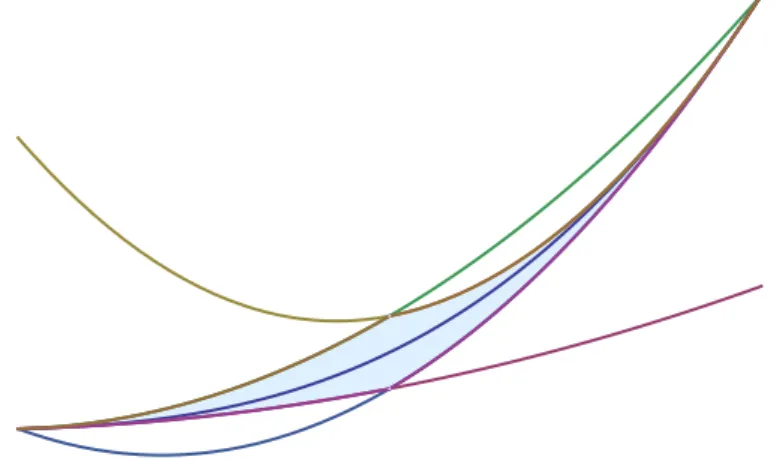
Figure 1. The cell Ck(a, b) betweenγk(a) (left endpoint) and γk(b) (right endpoint), k odd, shaded with blue. The curve Γk runs in the middle of the cell. The lower boundary consists of max{Φk(a),Ψk(b, a)}, the upper boundary is defined by min{Ψk(a, b),Φk(b)}.
Let us elaborate on thek>2 case (see Figure 1) . Whenkis even, the lower boundary of Ck(a, b) consists of two arcs: Φk(a) fora6x6(a+b)/2, and Φk(b) for (a+b)/26x6b.
The upper boundary again consists of two arcs: Ψk(a, b) fora6x6(a+b)/2, and Ψk(b, a)
for (a+b)/2 6 x 6 b (for k = 2, these coincide with each other). When k is odd, the lower and upper boundaries of Ck(a, b) are the same as in the even case; however, for (a+b)/26x6b, Φk(b) is the upper boundary, while Ψk(b, a) is the lower boundary. Thus, in any case, γk(a) and γk(b) are two opposite vertices of Ck(a, b), and other two vertices both have x-coordinates (a+b)/2.
The importance of the cell Ck(a, b) is given by the following statement.
Lemma 3.4. Let k>1, and 06a < b. The set of points p in the plane for which (γk(a)◦k, p, γk(b)◦k)
is a k-monotone chain is exactly Ck(a, b).
Proof. We prove the statement first assuming a >0. The case a= 0 may be obtained by a standard limit argument.
Let Φi,k(a, b, xk) be the polynomial defined by (8) for f(x) =xk. By comparing deriva- tives, we obtain that for every 16i6k+ 1,
(11) Φi,k(a, b, xk) =xk−(x−a)i−1(x−b)k+1−i.
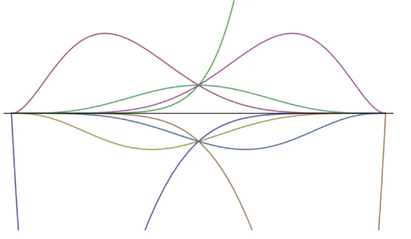
By Lemma 3.2, our goal is to determine the intersection of the regions above Φi,k(a, b, xk) for i = k+ 1, k−1, k−3, . . . ,1 + mod(k,2) and the regions below Φi,k(a, b, xk) for i = k, k−2, k−4, . . . ,2−mod(k,2) (see Figure 2). Thus, we have to determine
i≡k+1(mod 2)max
16i6k+1
Φi,k(a, b, xk) and
i≡k(mod 2)min
16i6k+1
Φi,k(a, b, xk)
for every x∈[a, b]. By (11), we obtain that for x∈[a,(a+b)/2], the above extrema occur when i=k+ 1, and i=k, respectively, while for x ∈[(a+b)/2, b], the extrema are taken when i= 1,2. Therefore, the boundary ofCk(a, b) is constituted by the polynomials of the
form (9) and (10).
Figure 2. Graphs of the polynomials xk−Φi,k(a, b, xk), 1 6 i 6 k+ 1, plotted between aand b, in thek= 7 case.
The next lemma states that not only Ck(a, b) is the location of thek-monotone chains, but given two k-monotone chains in neighboring cells, we may concatenate them.
Lemma 3.5. Assume 06a < b < c, and that the pointsp1, . . . , pl and pl+1, . . . , pm are so that (γk(a)◦k, p1, . . . , pl, γk(b)◦k) and (γk(b)◦k, pl+1, . . . , pm, γk(c)◦k) are k-monotone chains in Ck(a, b) and Cb,c, respectively. Then
(γk(a)◦k, p1, . . . , pm, γk(c)◦k) is a k-monotone chain in Ck(a, c).
Proof. By the remark following Lemma 1.7,
(γk(a)◦k, p1, . . . , pl, γk(b)◦k, pl+1, . . . , pm, γk(c)◦k)
is ak-monotone chain. By the transitivity property provided by Lemma 1.7, we may delete from this chain any point, still maintaining k-monotonicity. Therefore,
(γk(a)◦k, p1, . . . , pl, γk(b)◦(k−1), pl+1, . . . , pm, γk(c)◦k)
is also k-monotone. By iterating the erasure process, we finally erase all copies of γk(b),
yielding the statement.
Next, we introduce a transformation mapping Ck(a, b) to Ck(c, d) which preserves k- monotonicity, showing the equivalence of the cellsCk(a, b) with respect to problems regard- ing k-monotone chains.
Let 0< a < b and 0< c < d, and define the transformation Ta,b,c,d:R2 →R2 by (12) Ta,b,c,d(x, y) = c+ (x−a)d−c
b−a,
c+ (x−a)d−c b−a
k
+ (y−xk)
d−c b−a
k! . Lemma 3.6. For any 0< a < b and 0< c < d, the map Ta,b,c,d preservesk-monotonicity, keeps Γk fixed, and maps the uniform distribution onCk(a, b) onto the uniform distribution on Ck(c, d).
Proof. Notice that
Ta,b,c,d(a+t(b−a),(a+t(b−a))k+ ˜y) = c+t(d−c),(c+t(d−c))k+ ˜y
d−c b−a
k! . Thus, it is immediate that Ta,b,c,d(Γk) = Γk (as this corresponds to the case ˜y = 0). On the boundary of Ck(a, b), ˜y is either±(t(b−a))k,±((1−t)(b−a))k,±tk−1(1−t)(b−a)k, or±t(1−t)k−1(b−a)k, which are mapped to the same expressions with (d−c) in place of (b−a). Therefore, Ta,b,c,d mapsCk(a, b) onto Ck(c, d) by mapping the boundary curves to the corresponding ones. Measure invariance is seen by writing
Ta,b,c,d =G−1k ◦A◦Gk,
where Gk : (x, y) 7→ (x, y−xk), and A is an affine map. Thus, it only remains to check the invariance of k-monotonicity under Ta,b,c,d. To this end, we may write Ta,b,c,d as the composition of three maps:
Ta,b,c,d=T0,d−c,c,d◦T0,b−a,0,d−c◦Ta,b,0,b−a.
Assumef(x) has the formf(x) =xk+g(x), thenf(k)(x) =k! +g(k)(x). The first and third of the above maps do keep this derivative fixed, as g(x) is preserved by them. Finally, the map T0,b−a,0,d−c is a linear map scaling the x and y coordinates independently, therefore, it preserves the sign of the derivatives. Therefore, using Definition 1.4, Ta,b,c,d preserves positivity of (k+ 1)-tuples, hence it also preserves positivity.
We conclude this section by calculating the area of the base cellCk(a, b). By (9), (10) and the discussion afterwards, the distance between the upper and lower boundary of Ck(a, b) is (x−a)k−1(b−x). Therefore,
A(Ck(a, b)) =
Z (a+b)/2
a
(x−a)k−1(b−a)dt+ Z b
(a+b)/2
(b−x)k−1(b−a)dt
= (b−a)k+1 k2k−1 . (13)
4. The Poisson model
In order to make the problem more approachable, in this section we switch to thePoisson model, that has by now became an industry standard (see e.g. [18]).
Let Π be a planar homogeneous Poisson process with intensity 1. Given any domain D of area A(D) in the plane, the number of points of Π in D has Poisson distribution with parameter A(D). That is, its probability mass function is given by
(14) P(|D∩P i|=k) = A(D)ke−A(D)
k! ,
and its expectation is A(D).
We are going to use the following standard tail estimate for Poisson random variables, see Proposition 1 of [12]. Assume that Xhas Poisson distribution with parameterλ. Then (15) P(X >m)6 m+ 1
m+ 1−λP(X =k) = m+ 1
m+ 1−λe−λλm m!.
For arbitrary 0 6 a < b, let NΠk(a, b) be the cardinality of Π∩Ck(a, b). By (13) and (14), NΠk(a, b) has a Poisson distribution with parameter (and mean) (b−a)k+1/(k2k−1).
Moreover, conditioning on the eventNΠk(a, b) =N, the joint distribution of the points of Π falling in Ck(a, b) is the same as the joint distribution ofN i.i.d. uniform points inCk(a, b).
As the analogue of Definition 2.1, we introduce
Definition 4.1. Let MkΠ(a, b) be the set of all chains(p1, . . . , pm)⊂Π∩Ck(a, b) so that (16) (γk(a)◦k, p1, p2, . . . , pm, γk(b)◦k)
is ak-monotone chain. Furthermore, letLk(a, b)denote the maximal cardinality of elements of MkΠ(a, b).
By Lemma 3.6 and the invariance property of the Poisson process, the distribution of Lk(a, b) depends solely on (b−a); therefore, the results below involving Lk(0, n) remain also valid for the general variables Lk(a, b).
Next, we establish the link between the Poisson and the uniform models. By (13), the area of Ck(0, n) is nk+1/(k2k−1), therefore, NΠk(0, n) has a Poisson distribution with parameter nk+1/(k2k−1). On the other hand, let us denote by Nnk the number of points of Xn inCk(0,1). Then, Nnkhas binomial distribution with parametersnand 1/(k2k−1), and its mean is n/(k2k−1). Standard Chernoff type concentration estimates for binomial and Poisson random variables (see e.g. Chapter 2 of [9]) yield the following quantitative bound.
Proposition 4.2. For any k>1, and for any c >0, P |NΠk(0, n)−Nnkk+1|> c
r nk+1 k2k−1
!
<4e−c2/3 holds for every sufficiently large n.
This also implies that the random variable Lk(0, n) is a good approximation of Lknk+1. Applying Proposition 4.2 with c= εn(k+1)/2 allows us to transfer the statement of Theo- rem 2.2 to the Poisson model. We are going to prove the following theorem, which readily implies Theorem 2.2.
Theorem 4.3. For any k>1, there exists a positive constant αk so that
(17) lim
n→∞n−1ELk(0, n) =αk. Furthermore, n−1Lk(0, n)→αk almost surely, as n→ ∞.
First, we need an upper bound on ELk(0, n). In the uniform model for k = 2, this is fairly easy to establish. The probability that a random chain of lengthn is convex may be calculated exactly [8], based on a beautiful argument of Valtr [22]. The probability that n uniform independent random points in the unit square form a convex chain is exactly
1 n!(n+ 1)!.
The calculation is based on rearranging convex chains while keeping the underlying proba- bility space invariant. Unfortunately, this approach brakes down for larger values ofk, and thus, such a sharp result does not hold in the more general setting. However, we may still prove that the probability of the existence of very long k-monotone chains is minuscule.
Lemma 4.4. For every k>1 there exists a constant ck so that
(18) ELk(0, n)< ckn
holds for every n>1.
Proof. As the statement is known for the casesk= 1 andk= 2, we may assume thatk>3.
Also, it is sufficient to prove (18) for sufficiently large values of n. Let C be a constant whose value we are going to specify later. Set N =nk+1. As we noted before,NΠk(0, n) has Poisson distribution with parameter nk+1/(k2k−1). Therefore, using (15),
ELk(0, n) = Z ∞
0
P(Lk(0, n)>x)dx 6Cn+
Z N
Cn
P(Lk(0, n)>x)dx+ Z ∞
N
P(Lk(0, n)>x)dx 6Cn+NP(Lk(0, n)>Cn) +
Z ∞
N
P(NΠk(0, n)>x)dx 6Cn+NP(Lk(0, n)>Cn) + 2
∞
X
i=N
P(NΠk(0, n) =i) 6Cn+NP(Lk(0, n)>Cn) + 1
4N . (19)
Thus, it suffices to show that for suitably large C (depending on konly), P(Lk(0, n)>Cn) =o(n−k).
Call ak-monotone chain in Π∩Ck(0, n)longif its cardinality is at leastCn. To every such long k-monotone chain C we assign its skeleton as follows. Assume that C ={p1, . . . , pm}
(with the points ordered according to theirx-coordinates), wherem>Cn. Then skel (C) ={γk(0)◦k, pbm
nc, p2bm
nc, . . . , pn−1bm
nc, γk(n)◦k}
=:{γk(0)◦k, s1, . . . , sn−1, γk(n)◦k}, (20)
that is,si=pibm/ncfor every i= 1, . . . , n−1. Also, setsi =γk(0) for i60 andsj =γk(n) for j>n. Any long chain is cut intonintervals of length at least C by its skeleton.
The free part of the skeleton is a chain of length n−1 contained in Ck(0, n). The distribution of the long chains in Π∩Ck(0, n) induces a probability distribution µ on the space of skeletons. By the law of total probability,
P(Lk(0, n)>Cn) = Z
P(∃a longk-monotone chainC |skel (C) =S)dµ(S),
where the integral is taken over the space of possible skeleta. Thus, (19), implies (18) as long as
P(∃ a longk-monotone chainC |skel (C) =S)< o(n−k)
holds true for every possible skeletonS, with the constants of the asymptotic estimate being independent of S. This is what we are going to prove.
Let us now fix S of the form (20) and assume that C is a long k-monotone chain with skel (C) =S. Let p ∈ C \skel (C). For any point u∈ R2, letx(u) denote its x-coordinate.
There exists a unique index i so that x(p) ∈ [x(si), x(si+1)]. Then, by Definition 1.4 of k-monotone chains, the (k+ 1)-tuples
(si−k+1, si−k+2, . . . , si, p) and
(si−k+2, si−k+3, . . . , si, p, si+1)
are positive. Let P1 be the unique polynomial of degree k−1 whose graph contains the pointssi−k+1, si−k+2, . . . , si, and similarly, let P2 be the unique polynomial of degreek−1 whose graph contains the points si−k+2, si−k+3, . . . , si, si+1, possibly using the extended definition for multisets discussed in Section 1. That is, if γk(0) appears with multiplicityβ among the nodes for Pi fori= 1 or 2, than the derivatives up to orderβ−1 ofPi at 0 are required to agree with those of xk at 0.
Lemma 3.1 and its generalization to multisets implies that the point plies in the region Ri bounded by the graphs of the polynomials P1 and P2 over the interval [x(si), x(si+1)].
Lemma 1.5 and formula (2) shows that P1(x)−P2(x) =
∆k−1(si−k+1, si−k+2, . . . , si)
−∆k−1(si−k+2, si−k+3, . . . , si, si+1)k−1Y
j=1
(x−x(si+1−j)). Therefore,
A(Ri) =
Z x(si+1) x(si)
|P1(x)−P2(x)|
6 x(si+1)−x(si)
x(si+1)−x(si−k+2)k−1
Di
6 x(si+1)−x(si−k+2)k
Di (21)
with
Di= ∆k−1(si−k+2, si−k+3, . . . , si, si+1)−∆k−1(si−k+1, si−k+2, . . . , si).
Since
n−1
X
i=0
x(si+1)−x(si−k+2) =
k−2
X
j=0
x(sn−j)−x(s−j)< kn, there are at least (2n)/3 indicesiin the interval [0, n−1] so that
(22) x(si+1)−x(si−k+2)63k .
On the other hand, thek-monotonicity ofCimplies that (∆k−1(si−k+1, si−k+2, . . . , si))n+k−1i=0 is a monotone increasing sequence, which, by (4), satisfies
∆k−1(s−k+1, s−k+2, . . . , s0) = 0 and
∆k−1(sn, sn+1, . . . , sn+k−1) =kn .
Thus, there exist at least (2n)/3 indices j in the interval [0, n−1] so that (23) ∆k−1(sj−k+1, sj−k+2, . . . , sj)63k.
Combining (22) and (23) with (21), we obtain that there at leastn/3 indices i∈[0, n−1]
so that
A(Ri)6(3k)k+1.
In order for C to be long, each of these regions must contain at leastC points of Π. Pick such a region R. By (15) and Stirling’s approximation,
P |R∩Π|>C
62 e(3k)k+1 C
!C
holds for any sufficiently largeC. Therefore, for any givenε >0, there exists a correspond- ing C so that the above probability is bounded above byε. For that choice of C,
P(∃ a longk-monotone chainC |skel (C) =S)6
n−1
Y
i=0
P |Ri∩Π|>C 6εn/3,
where the independence property of the Poisson process is used in the first inequality. The proof is finished by noting that he above expression is of order o(n−k) for sufficiently small values of ε, and all the above estimates depend on k only.
5. Expectation and concentration estimates
In this section, we show that the order of magnitude of the length of the longest k- monotone chains among n random points is n1/(k+1). We are going to prove this in the Poisson model, Theorem 4.3, which implies Theorem 2.2 of the uniform model. The proof builds on Kingman’s subbaditive ergodic theorem. Below, we present a version of it along with an important extension by Liggett.
Theorem 5.1 (Kingman’s subadditive ergodic theorem with Liggett’s extension [14, 15]).
Assume Xn,m,n, m∈N, is a family of random variables satisfying the following conditions:
S1) Xl,n6Xl,m+Xm,n whenever 06l < m < n;
S2) For every s > 0 integer, the joint distributions of the process {Xm+s,n+s} are the same as those of {Xm,n};
S3) For each n, E|X0,n|<∞ andEX0,n >−cnfor some constant c.
Then
γ = lim
n→∞
EX0,n
n exists,
X = lim
n→∞
X0,n n exists almost surely, and EX=γ.
Furthermore, if the stationary sequences (Xin,(i+1)m)∞i=1 are ergodic for any m>1, then X =γ almost surely.
Proof of Theorem 4.3. We show that Conditions S1), S2) and S3) of Theorem 5.1 hold for the family of random variablesXm,n :=−Lk(n, m),n, m∈N, see Definition 4.1. Lemma 3.5 shows that
Lk(a, c)>Lk(a, b) +Lk(b, c)
for every 06 a < b < c, showing the validity of S1). The invariance property S2) follows from Lemma 3.6. Finally, S3) is implied by Lemma 4.4.
Therefore, we may apply Theorem 5.1 to obtain that ELk(0, n) ≈αkn with some pos- itive constant βk. Moreover, (Lk(in,(i+ 1)n)∞i=1 is a sequence of independent, identically distributed random variables, hence it is ergodic. Therefore, n−1Lk(0, n) converges to αk
almost surely.
Theorem 4.3 and Proposition 4.2 implies that Lkn
n1/(k+1) →αk almost surely, proving Theorem 2.2.
Next, we derive a lower bound on the constant αk of (17).
Proof of Proposition 2.3. We are going to prove the statement in the Poisson model by showing that for sufficiently large n,
ELk(0, n)> n 6 holds.
Set ai = 3ifor everyi∈[0,bn/3c]. By (13), the area ofCk(ai, ai+1) (see Definition 3.3) is
A(Ck(ai, ai+1)) = 3k k2k−1 >1.
Since the number of points of Π in Ck(ai, ai+1) has Poisson distribution with parameter A(Ck(ai, ai+1)),
P(|Π∩Ck(ai, ai+1)|= 0) =e−A(Ck(ai,ai+1))< 1 e.
Let Y be the number of cells of the form Ck(ai, ai+1) in which Π has at least one point.
Then Y ∼B(bn3c, p) with p >1−1/e >1/2. Let λ:= EY, then λ > n(1−1/e)/3. By a standard Chernoff-type bound for binomial random variables (see Theorem A.1.12 of [2]),
P
Y 6λ−cp λlogλ
< λ−c2/2. Therefore, for sufficiently large n,
(24) P(Y > n/6)≈1.
Let us now take a point p of Π in each of the non-empty cells, and let S ={s1, . . . , sY} be the collection of these points ordered with respect to their x-coordinates. By the con- struction,
γk(0)◦k, s1, γk(a1)◦k, s2, . . . , γk(abn/3c)◦k, γk(n)◦k
is a k-monotone chain, where each si is placed in its corresponding interval so that we obtain a chain. By repeatedly applying Lemma 3.5, we deduce that
γk(0)◦k, s1, s2, . . . , sY, γk(n)◦k
is also a k-monotone chain. Therefore, Lk(0, n) > Y. The proof is finished by referring
to (24), which shows that ELk(0, n)>n/6.
We finish this section by establishing the exponential concentration estimate for Lkn. Theorem 2.4 is straightforward consequence of Talagrand’s strong concentration inequality.
Theorem 5.2 (Talagrand [20]). Suppose Y is a real-valued random variable on a product probability space Ω⊗n, and that Y is 1-Lipschitz with respect to the Hamming distance, meaning that
|Y(x)−Y(y)|61
whenever x andy differ in one coordinates. Moreover assume that Y isf-certifiable. This means that there exists a function f :N→ N with the following property: for every x and b with Y(x) >b there exists an index set I of at most f(b) elements, such that Y(y) >b holds for every y agreeing with x on I. Let m denote the median of Y. Then for every s >0 we have
P(Y 6m−s)62 exp −s2 4f(m)
!
and
P(Y >m+s)62 exp −s2 4f(m+s)
! .
The conditions of Theorem 5.2 are clearly satisfied by the random variable Lkn with the certificate function f(b) =b, by fixing the points of the longest k-monotone chain in Xn. Since Lkn6n, exponential concentration ensures that the mean and the median are within a distance of O(n1/2(k+1)) of each other. Thus, in the above estimates, m ≈ αkn1/(k+1), and setting s=εn1/2(k+1), we obtain Theorem 2.4.
The same proof yields the analogous concentration estimate forLk(0, n):
Theorem 5.3. For every k>1, and for every ε >0, P
|Lk(0, n)−ELk(0, n)|> ε√ n
65e−ε2/5αk. holds for every sufficiently large n.
Summarizing the results proved in this section, we showed that Lkn is a random variable exponentially concentrated in a neighbourhood of radius O(n1/2(k+1)) around its mean, which converges to αkn1/(k+1).
References
[1] D. Aldous and P. Diaconis, Longest increasing subsequences: from patience sorting to the Baik-Deift- Johansson theorem.Bull. Amer. Math. Soc.36(1999), 413–432.
[2] N. Alon, J. Spencer,The probabilistic method.2nd ed. John Wiley & Sons, New York (2000).
[3] G. Ambrus,Analytic and Probabilistic Problems in Discrete Geometry. Ph.D. Thesis, University College London, 2009.
[4] G. Ambrus, Longest convex chains and subadditive ergodicity.In: G. Ambrus, K.J. B¨or¨oczky, and Z.
F¨uredi (eds.), Discrete geometry and convexity, in honour of Imre B´ar´any. Typotex, Budapest (2017).
[5] G. Ambrus and I. B´ar´any, Longest convex chains,Random Structures Algorithms35 (2009), no. 2., 137–162.
[6] J. Baik, P. Deift, and K. Johansson, On the distribution of the length of the longest increasing subse- quence of random permutations. J. Amer. Math. Soc.12(1999), 1119–1178.
[7] I. B´ar´any,Random points and lattice points in convex bodies.Bull. Amer. Math. Soc.45(2008), no. 3., 339–365.
[8] I. B´ar´any, G. Rote, W. Steiger, and C.-H. Zhang, A central limit theorem for convex chains in the square.Discrete Comput. Geom.23(2000), 35–50.
[9] S. Boucheron, G. Lugosi, and P. Massart, Concentration Inequalities: A Nonasymptotic Theory of Independence.Oxford University Press, Oxford, 2013.
[10] M. Eli´aˇs and J. Matouˇsek,Higher order Erd˝os-Szekeres theorems.Adv. Math.244(2013), 1–15.
[11] J. Fox, J. Pach, B. Sudakov, and A. Suk,Erd˝os–Szekeres-type theorems for monotone paths and convex bodies.Proc. London Math. Soc105(2012), no. 5., 953–982.
[12] P. W. Glynn,Upper bounds on Poisson tail probabilities.Oper. Res. Lett.6(1987), no. 1, 9–14.
[13] J.M. Hammersley, A few seedlings of research. In: L. M. LeCam, J. Neyman, and E.L. Scott (eds.), Proceedings of the Sixth Berkeley Symposium on Mathematical Statistics and Probability, Volume 1:
Theory of Statistics. University of California Press (1972), 345–394.
[14] J.F.C. Kingman,Subadditive ergodic theory, Ann. Prob.1(1973), no. 6., 883–909.
[15] T.M. Liggett,An improved subadditive ergodic theorem.Ann. Probab.13(1985), 1279–1285.
[16] B.F. Logan and L.A. Shepp,A variational problem for random Young tableaux.Adv. Math.26(1977), 206–222.
[17] G.M. Phillips,Interpolation and approximation by polynomials. Springer Verlag, Berlin (2003).
[18] D. Romik,The surprising mathematics of longest increasing subsequences. Cambridge University Press (2014).
[19] R. Schneider and W. Weil,Stochastic and Integral Geometry.Springer Verlag (2008).
[20] M. Talagrand, A new look at independence.Ann. Probab.24(1996), 1–34.
[21] S. Ulam, Monte Carlo calculations in problems of mathematical physics. In: E.F. Beckenbach (ed.), Modern Mathematics For the Engineer, Second Series. McGraw-Hill (1961), 261–281.
[22] P. Valtr, The probability that n points are in convex position. Discrete Comput. Geom. 13 (1995), 637–643.
[23] A.M. Vershik and S.V. Kerov, Asymptotics of the Plancherel measure of the symmetric group and the limiting form of Young tables. Soviet Math. Dokl., 18 (1977), 527–531. Translation of Dokl. Acad.
Nauk. SSSR233(1977), 1024–1027.